UR-1556
ER/40685/925
DTP/98/82
November 1998
A BFKL MONTE CARLO APPROACH TO JET PRODUCTION
AT HADRON-HADRON AND LEPTON-HADRON COLLIDERS

The production of a pair of jets with large rapidity separation in hadron-hadron collisions, and of forward jets in deep inelastic scattering, can in principle be used to test the predictions of the BFKL equation. However in practice kinematic constraints lead to a strong suppression of BFKL effects for these processes. This is illustrated using a BFKL Monte Carlo approach.

1 Introduction

Fixed-order QCD perturbation theory fails in some asymptotic regimes where large logarithms multiply the coupling constant. In those regimes resummation of the perturbation series to all orders is necessary to describe many high-energy processes. The Balitsky-Fadin-Kuraev-Lipatov (BFKL) equation $\!{}^{{\bf?}}$ performs such a resummation for virtual and real soft gluon emissions in dijet production at large rapidity difference in hadron-hadron collisions (see Figure 1(a)) and in forward jet production in lepton-hadron collisions (Figure 1(b)). In the latter case, resummation leads to the characteristic BFKL rise in the forward jet cross section, $\hat{\sigma}\sim(x_{j}/x_{Bj})^{\lambda}$, with $\lambda=4C_{A}\ln 2\,\alpha_{s}/\pi\approx 0.5$. Similarly, in dijet production at hadron colliders BFKL resummation gives $\!{}^{{\bf?}}$ a subprocess cross section that increases with rapidity difference as $\hat{\sigma}\sim\exp(\lambda\Delta)$, where $\Delta$ is the rapidity difference of the two jets with comparable transverse momenta $p_{T1}$ and $p_{T2}$.

Experimental studies of these processes have recently begun at the Tevatron $p\bar{p}$ and HERA $ep$ colliders. Tests so far have been inconclusive; the data tend to lie between fixed-order QCD and analytic BFKL predictions. However the applicability of these analytic BFKL solutions is limited by the fact that they implicitly contain integrations over arbitrary numbers of emitted gluons with arbitrarily large transverse momentum: there are no kinematic constraints included. Furthermore, the implicit sum over emitted gluons leaves only leading-order kinematics, i.e. only the momenta of the ‘external’ particles are made explicit. The absence of kinematic constraints and energy-momentum conservation cannot, of course, be reproduced in experiments. While the effects of such constraints are in principle sub-leading, it is desirable to include them in predictions to be compared with experimental results. As we will see, kinematic constraints can affect predictions substantially.

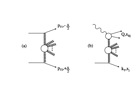
Figure 1: Schematic representation of (a) dijet production with large rapidity separation $\Delta$ in hadron–hadron collisions, and (b) forward jet production in deep inelastic scattering.

2 Monte Carlo Approach to BFKL Physics

The solution to this problem of lack of kinematic constraints in analytic BFKL predictions is to unfold the implicit sum over gluons to make the gluon sum explicit, and to implement the result in a Monte Carlo event generator $\!{}^{{\bf?},{\bf?}}$. This is achieved as follows. The BFKL equation contains separate integrals over real and virtual emitted gluons. We can reorganize the equation by combining the ‘unresolved’ real emissions — those with transverse momenta below some minimum value (in practice chosen to be small compared to the momentum threshold for measured jets) — with the virtual emissions. Schematically, we have

$$\int_{virtual}+\int_{real}=\int_{virtual+real,unres.}+\int_{real,res.}$$ (1)

We perform the integration over virtual and unresolved real emissions analytically. The integral containing the resolvable real emissions is left explicit.

We can then solve the BFKL equation by iteration, and we obtain a differential cross section that contains an explicit sum over emitted gluons along with the appropriate phase space factors. In addition, we obtain an overall form factor due to virtual and unresolved emissions. The subprocess cross section is

$$d\hat{\sigma}=d\hat{\sigma}_{0}\times\sum_{n\geq 0}f_{n}$$ (2)

where $f_{n}$ is the iterated solution for $n$ real gluons emitted and contains the overall form factor. It is then straightforward to implement the result in a Monte Carlo event generator. Emitted real (resolved) gluons appear explicitly, so that conservation of momentum and energy, as well as evaluation of parton distributions that multiply $d\hat{\sigma}$, is based on exact kinematics for each event. In addition, we include the running of the strong coupling constant. See $\!{}^{{\bf?}}$ for further details.

3 Dijet Production at Hadron Colliders

At hadron colliders, the BFKL increase in the dijet subprocess cross section with rapidity difference is unfortunately washed out by the falling parton distribution functions (pdfs). As a result, the BFKL prediction for the total cross section is simply a less steep falloff than obtained in fixed-order QCD, and tests of this prediction are sensitive to pdf uncertainties. A more robust pediction is obtained by noting that the emitted gluons (cf. Figure 1(a)) give rise to a decorrelation in azimuth between the two leading jets.$\!{}^{{\bf?},{\bf?}}$ This decorrelation becomes stronger as the rapidity difference $\Delta$ increases and more gluons are emitted. In lowest order in QCD, in contrast, the jets are back-to-back in azimuth and the (subprocess) cross section is constant, independent of $\Delta$.

This azimuthal decorrelation is illustrated in Figure 2 for dijet production at the Tevatron $p\bar{p}$ collider $\!{}^{{\bf?}}$, with center of mass energy 1.8 TeV and jet transverse momentum $p_{T}>20\ {\rm GeV}$. The azimuthal angle difference $\Delta\phi$ is defined such that that $\cos\Delta\phi=1$ for back-to-back jets. The solid line shows the analytic BFKl prediction. The BFKL Monte Carlo prediction is shown as crosses. We see that the kinematic constraints result in a less strong decorrelation due to suppression of emitted gluons, and we obtain improved agreement with preliminary measurements by the D$\emptyset$ collaboration $\!{}^{{\bf?}}$, shown as diamonds in the figure.

The azimuthal decorrelation can also be studied at the LHC $pp$ collider $\!{}^{{\bf?}}$, which has higher rapidity reach than the Tevatron. Figure 3 compares the decorrelation at the Tevatron for $p_{T}>20\ {\rm GeV}$ (dotted curve; same as crosses in Fig. 2) to that at the LHC for $p_{T}>20\ {\rm GeV}$ (solid curve) and $p_{T}>50\ {\rm GeV}$ (dashed curve). We see that at the LHC for $p_{T}>20\ {\rm GeV}$ the decorrelation is stronger and reaches to larger rapidities than the Tevatron. The LHC’s higher center of mass energy ($\sqrt{s}=14\ {\rm TeV}$) relative to $p_{T}$ threshold allows for more emitted gluons, and the characteristic BFKL effects are more pronounced. For the perhaps more realistic LHC $p_{T}$ threshold of $50\ {\rm GeV}$, the kinematic suppression is more pronounced, but we still see a strong decorrelation. In all three curves we see the suppression of the decorrelation by the kinematic constraints as $\Delta$ approaches the kinematic limit, where the suppression of emitted gluons is so strong that the curve turns over and the correlation begins to return.

In addition to studying the azimuthal decorrelation, one can look for the BFKL rise in dijet cross section with rapidity difference by considering ratios of cross sections at different center of mass energies at fixed $\Delta$. The idea is to cancel the pdf dependence, leaving the pure BFKL effect. This turns out to be rather tricky $\!{}^{{\bf?}}$, because the desired cancellations occur only at lowest order, and the kinematic constraints strongly affect the predicted behavior, not only quantitatively but sometimes qualitatively as well $\!{}^{{\bf?},{\bf?}}$.

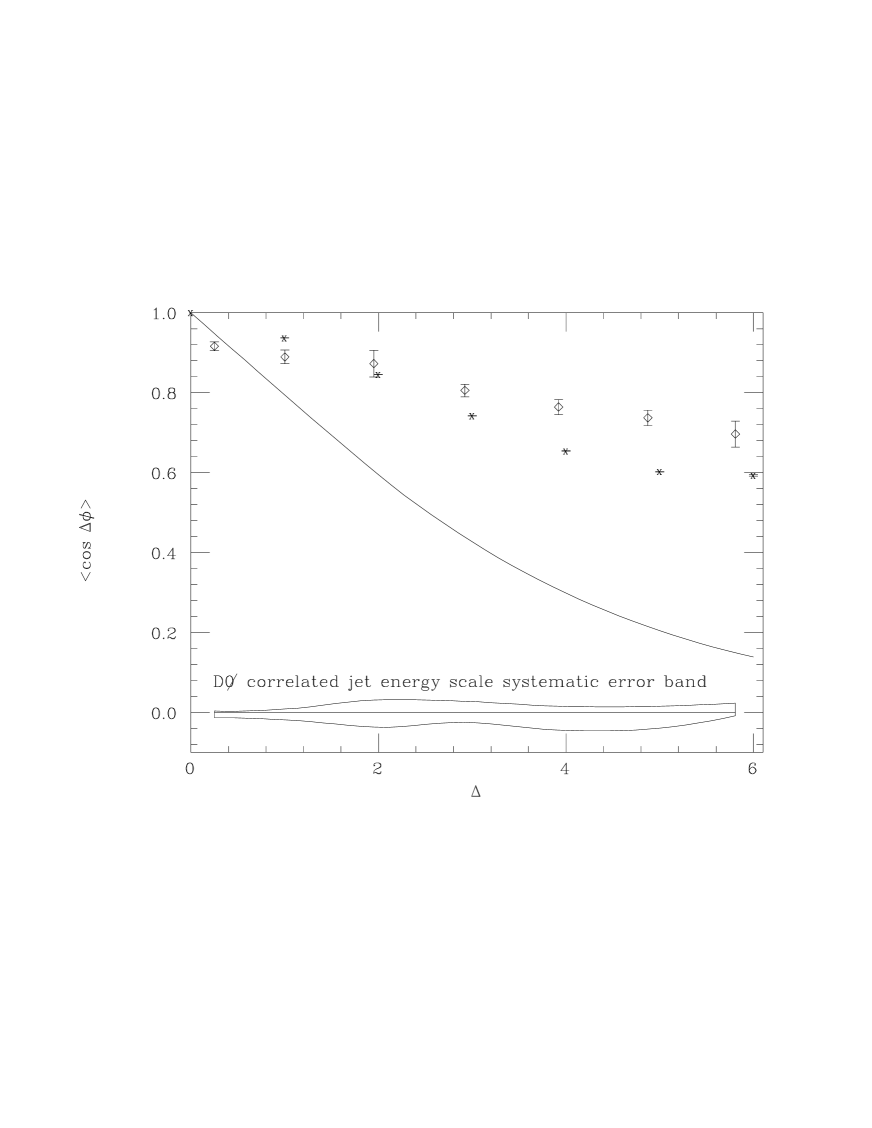
Figure 2: The azimuthal angle decorrelation in dijet production at the Tevatron as a function of dijet rapidity difference $\Delta$, for jet transverse momentum $p_{T}>20\ {\rm GeV}$. The analytic BFKL solution is shown as a solid curve and a preliminary D$\emptyset$ measurement $\!{}^{{\bf?}}$ is shown as diamonds. Error bars represent statistical and uncorrelated systematic errors; correlated jet energy scale systematics are shown as an error band.

Figure 3: The azimuthal angle decorrelation in dijet production at the Tevatron ($\sqrt{s}=1.8\;{\rm GeV}$) and LHC ($\sqrt{s}=14\;{\rm TeV}$) as a function of dijet rapidity difference $\Delta$. Dotted curve: Tevatron, $p_{T}>20\;{\rm GeV}$; solid curve: LHC, $p_{T}>20\;{\rm GeV}$; dashed curve: LHC, $p_{T}>50\;{\rm GeV}$.

4 Forward Jet Production at Lepton–Hadron Colliders

In deep inelastic scattering at lepton-hadron colliders, the production of forward jets $\!{}^{{\bf?}}$ is subject to the effects of multiple soft gluon emission just as in dijet production at hadron colliders. Now the large rapidity separation is between the current and forward jets; see Fig. 1(b). The BFKL equation resums such emissions, and it is relatively straightforward to adapt the dijet formalism to calculate the cross section for the production of a forward jet with a given $k_{T}$ and longitudinal momentum fraction $x_{j}\gg x_{\rm Bj}$. In fact there is a direct correspondence between the variables: $p_{T2}\leftrightarrow k_{T}$ and $\Delta\leftrightarrow\ln(x_{j}/x_{\rm Bj})$. In the DIS case the variable $p_{T1}$ corresponds to the transverse momentum of the $q\bar{q}$ pair in the upper ‘quark box’ part of the diagram. In practice this variable is integrated with the off–shell $\gamma^{*}g^{*}\to q\bar{q}$ amplitude such that $p_{T1}^{2}\sim Q^{2}$. As a result, it is appropriate to consider values of $k_{T}^{2}$ of the same order, and to consider the (formal) kinematic limit $x_{j}/x_{\rm Bj}\to\infty$, $Q^{2}$ fixed. In this limit we obtain the ‘naive BFKL’ prediction $\hat{\sigma}_{\rm jet}\sim(x_{j}/x_{\rm Bj})^{\lambda}$, the analog of $\hat{\sigma}_{jj}\sim\exp(\lambda\Delta)$.

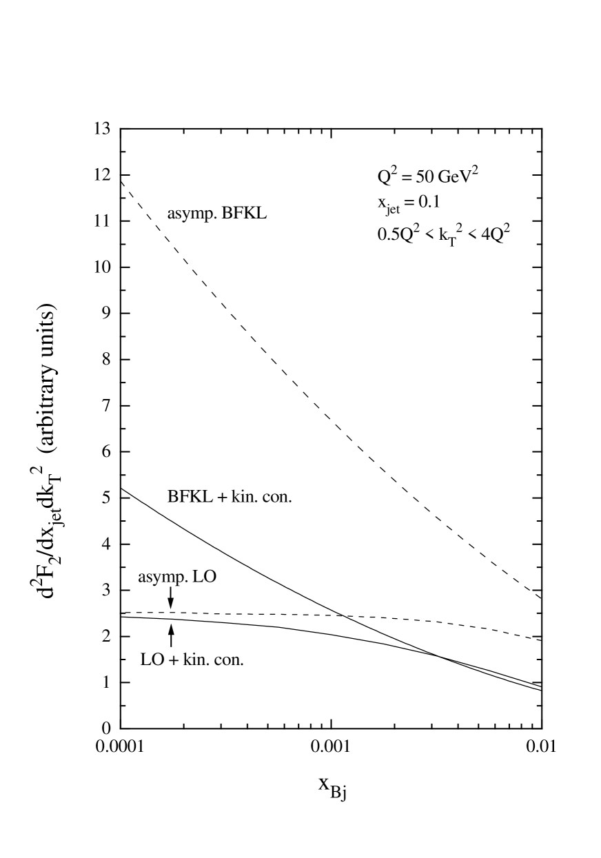
Figure 4: Differential structure function for forward jet production in $ep$ collisions at HERA. The curves are described in the text.

Figure 4 shows the differential structure function $\partial^{2}F_{2}/\partial x_{j}\partial k_{T}^{2}$ as a function of $x_{\rm Bj}$ at HERA, with

$$x_{j}=0.1,\;\;\;Q^{2}=50\;{\rm GeV}^{2},\;\;\;Q^{2}/2<k_{T}^{2}<4Q^{2}.$$ (3)

The lower dashed curve is the QCD leading–order prediction from the process $\gamma^{*}{\cal G}\to q\bar{q}{\cal G}$, with ${\cal G}=g,q$, with no overall energy–momentum constraints. This is the analog of the $\hat{\sigma}_{jj}\to\$constant prediction for dijet production. Note that here the parton distribution function at the lower end of the ladder is evaluated at $x=x_{j}$, independent of $x_{\rm Bj}$. In practice, when $x_{\rm Bj}$ is not small we have $x>x_{j}$ and the cross section is suppressed, as indicated by the lower solid curve in Fig. 4. The upper dashed curve is the asymptotic BFKL prediction with the characteristic $(x_{j}/x_{\rm Bj})^{\lambda}$ behavior. Finally the upper solid line is the prediction of the full BFKL Monte Carlo, including kinematic constraints and pdf dependence. We see a significant suppression of the cross section. We emphasise that Fig. 4 corresponds to ‘illustrative’ cuts and should not be directly compared to the experimental measurements. Nevertheless, the BFKL–MC predictions do appear to follow the general trend of the H1 and ZEUS measurements $\!{}^{{\bf?}}$. A more complete study, including realistic experimental cuts and an assessment of the uncertainty in the theoretical predictions, is under way and will be reported elsewhere $\!{}^{{\bf?}}$.

5 Conclusions

In summary, we have developed a BFKL Monte Carlo event generator that allows us to include the subleading effects such as kinematic constraints and running of $\alpha_{s}$. We have applied this Monte Carlo to dijet production at large rapidity separation at the Tevatron and LHC, and to forward jet production at HERA; the latter work is currently being completed. We found that kinematic constraints, though nominally subleading, can be very important. In particular they lead to suppression of gluon emission, which in turn suppresses some of the behavior that is considered to be characteristic of BFKL physics. It is clear therefore that reliable BFKL tests can only be performed using predictions that incorporate kinematic constraints.

References

References

- [1] L.N. Lipatov, Sov. J. Nucl. Phys. 23 (1976) 338; E.A. Kuraev, L.N. Lipatov and V.S. Fadin, Sov. Phys. JETP 45 (1977) 199; Ya.Ya. Balitsky and L.N. Lipatov, Sov. J. Nucl. Phys. 28 (1978) 822.
- [2] A.H. Mueller and H. Navelet, Nucl. Phys. B282 (1987) 727.
- [3] L.H. Orr and W.J. Stirling, Phys. Rev. D56 (1997) 5875.
- [4] C.R. Schmidt, Phys. Rev. Lett. 78 (1997) 4531.
- [5] V. Del Duca and C.R. Schmidt, Phys. Rev. D49 (1994) 4510; W.J. Stirling, Nucl. Phys. B423 (1994) 56; V. Del Duca and C.R. Schmidt, Phys. Rev. D51 (1995) 215; V. Del Duca and C.R. Schmidt, Nucl. Phys. Proc. Suppl. 39BC (1995) 137; preprint DESY 94-163 (1994), presented at the 6th Rencontres de Blois, Blois, France, June 1994.
- [6] D collaboration: S. Abachi et al., Phys. Rev. Lett. 77 (1996) 595; D collaboration: presented by Soon Yung Jun at the Hadron Collider Physics XII Conference, Stony Brook, June 1997.
- [7] L.H. Orr and W.J. Stirling, Phys. Lett. B436 (1998) 372.
- [8] L.H. Orr and W.J. Stirling, Phys. Lett. B429 (1998) 135.
- [9] A.H. Mueller, Nucl. Phys. B, Proc. Suppl. 18 C (1991) 125; W.K. Tang, Phys. Lett. B278 (1991) 363; J. Bartels et al., Z. Phys. C54 (1992) 635; Phys. Lett. B309 (1993) 400; Phys. Lett. B384 (1996) 300; J. Kwieciński, A.D.Martin and P.J. Sutton, Phys. Rev. D46 (1992) 921; Nucl. Phys. B, Proc. Suppl. 29A (1992) 67.
- [10] H1 collaboration, these proceedings; ZEUS collaboration, these proceedings.
- [11] L.H. Orr and W.J. Stirling, in preparation.