Precision test of the Standard Model from
Z physics
Frederic Teubert
European Laboratory for Particle Physics (CERN),
CH-1211 Geneva 23, Switzerland
E-mail: frederic.teubert@cern.ch

The measurements performed at LEP and SLC have substantially improved the precision of the test of the Minimal Standard Model. The precision is such that there is sensitivity to pure weak radiative corrections. This allows to indirectly determine the top mass ($\mathrm{m}_{\mathrm{t}}$=161$\pm$8 GeV), the W-boson mass ($\mathrm{M}_{\mathrm{W}}$=80.37$\pm$0.03 GeV), and to set an upper limit on the the Higgs boson mass of 262 GeV at 95% confidence level.

Invited talk presented at the IVth International Symposium
on Radiative Corrections (RADCOR 98),
Barcelona, Spain, Catalonia, September 8-12, 1998.

Abstract

The measurements performed at LEP and SLC have substantially improved the precision of the test of the Minimal Standard Model. The precision is such that there is sensitivity to pure weak radiative corrections. This allows to indirectly determine the top mass ($\mathrm{m}_{\mathrm{t}}$=161$\pm$8 GeV), the W-boson mass ($\mathrm{M}_{\mathrm{W}}$=80.37$\pm$0.03 GeV), and to set an upper limit on the the Higgs boson mass of 262 GeV at 95% confidence level.

1 Introduction

In the context of the Minimal Standard Model (MSM), any ElectroWeak (EW) process can be computed at tree level from $\alpha$ (the fine structure constant measured at values of $q^{2}$ close to zero), $\mathrm{M}_{\mathrm{W}}$ (the W-boson mass), $\mathrm{M}_{\mathrm{Z}}$ (the Z-boson mass), and $\mathrm{V}_{\mathrm{jk}}$ (the Cabbibo-Kobayashi-Maskawa flavour-mixing matrix elements).

When higher order corrections are included, any observable can be predicted in the “on-shell” renormalization scheme as a function of:

$$O_{i} = f_{i}(\alpha,\alpha_{\mathrm{s}},\mathrm{M}_{\mathrm{W}},\mathrm{M}_{\mathrm{Z}},\mathrm{M}_{\mathrm{H}},\mathrm{m}_{\mathrm{f}},\rm{V}_{\rm{jk}})$$

and contrary to what happens with “exact gauge symmetry theories”, like QED or QCD, the effects of heavy particles do not decouple. Therefore, the MSM predictions depend on the top mass ($\mathrm{m}^{2}_{\mathrm{t}}/\mathrm{M}^{2}_{\mathrm{Z}}$) and to less extend to the Higgs mass (log($\mathrm{M}^{2}_{\mathrm{H}}/\mathrm{M}^{2}_{\mathrm{Z}}$)), or to any kind of “heavy new physics”.

The subject of this letter is to show how the high precision achieved in the EW measurements from $\mathrm{Z}$ physics allows to test the MSM beyond the tree level predictions and, therefore, how this measurements are able to indirectly determine the value of $\mathrm{m}_{\mathrm{t}}$ and $\mathrm{M}_{\mathrm{W}}$, to constrain the unknown value of $\mathrm{M}_{\mathrm{H}}$, and at the same time to test the consistency between measurements and theory. At present the uncertainties in the theoretical predictions are dominated by the precision on the input parameters.

1.1 Input Parameters of the MSM

The W mass is one of the input parameters in the “on-shell” renormalization scheme. It is known with a precision of about 0.07%, although the usual procedure is to take $G_{\mu}$ (the Fermi constant measured in the muon decay) to predict $\mathrm{M}_{\mathrm{W}}$ as a function of the rest of the input parameters and use this more precise value.

Therefore, the input parameters are chosen to be:

$$\rm{Input~{}Parameter} \rm{Value} \rm{Relative~{}Uncertainty}$$

$$\alpha^{-1}(\mathrm{M}^{2}_{\mathrm{Z}})= 128.896(90) 0.07\%$$

$$\alpha_{\mathrm{s}}(\mathrm{M}^{2}_{\mathrm{Z}})= 0.119(2) 1.7\%$$

$$G_{\mu}= 1.16639(2)\times 10^{-5}~{}\mathrm{GeV^{-2}} 0.0017\%$$

$$\mathrm{M}_{\mathrm{Z}}= 91.1867(21)~{}\mathrm{GeV} 0.0023\%$$

$$\mathrm{m}_{\mathrm{t}}= 173.8(50)~{}\mathrm{GeV} 2.9\%$$

$$\mathrm{M}_{\mathrm{H}}> 89.8~{}\mathrm{GeV}~{}@95\%~{}C.L.$$

Notice that the less well known parameters are $\mathrm{m}_{\mathrm{t}}$, $\alpha_{\mathrm{s}}$ and, of course, the unknown value of $\mathrm{M}_{\mathrm{H}}$. The next less well known parameter is $\alpha^{-1}(\mathrm{M}^{2}_{\mathrm{Z}})$, even though its value at $q^{2}\sim 0$ is known with an amazing relative precision of $4\times 10^{-8}$, ($\alpha^{-1}(0)=137.0359895~{}(61)$).

The reason for this loss of precision when one computes the running of $\alpha$,

$$\alpha^{-1}(\mathrm{M}^{2}_{\mathrm{Z}}) = \frac{\alpha^{-1}(0)}{1-\Pi_{\gamma\gamma}}$$

is the large contribution from the light fermion loops to the photon vacuum polarisation, $\Pi_{\gamma\gamma}$. The contribution from leptons and top quark loops is well calculated but for the light quarks non-perturbative QCD corrections are large at low energy scales. The method so far has been to use the measurement of the hadronic cross section through one-photon exchange, normalised to the point-like muon cross-section, R(s), and evaluate the dispersion integral:

$$\Re(\Pi^{\mathrm{had}}_{\gamma\gamma}) = \frac{\alpha\mathrm{M}^{2}_{\mathrm{Z}}}{3\pi}\Re\left(\int\frac{R(s^{\prime})}{s^{\prime}(s^{\prime}-\mathrm{M}^{2}_{\mathrm{Z}}+i\epsilon)}ds^{\prime}\right)$$ (1)

giving [1] $\Pi_{\gamma\gamma}=-0.0632\pm 0.0007$, the error being dominated by the experimental uncertainty in the cross section measurements.

Recently, several new “theory driven” calculations [2] [3] have reduced this error by a factor of about 4.5, by extending the regime of applicability of Perturbative QCD (PQCD). This needs to be confirmed using precision measurements of the hadronic cross section at $\sqrt{s}\sim$ 1 to 7 GeV. The very preliminary first results from BESS II [4] seem to validate this procedure, being in agreement with the predictions from PQCD.

1.2 What are we measuring to test the MSM?

From the point of view of radiative corrections we can divide the $\mathrm{Z}$ measurements into three different groups: the $\mathrm{Z}$ total and partial widths, the partial width into b-quarks ($\Gamma_{\mathrm{b}}$), and the $\mathrm{Z}$ asymmetries ($\sin^{2}\theta_{\mathrm{eff}}$). For instance, the leptonic width ($\Gamma_{\mathrm{l}}$) is mostly sensitive to isospin-breaking loop corrections ($\Delta\rho$), the asymmetries are specially sensitive to radiative corrections to the $\mathrm{Z}$ self-energy, and $\mathrm{R}_{\mathrm{b}}$ is mostly sensitive to vertex corrections in the decay $\mathrm{Z}\rightarrow b\bar{b}$. One more parameter, $\Delta r$, is necessary to describe the radiative corrections to the relation between $G_{\mu}$ and $\mathrm{M}_{\mathrm{W}}$.

The sensitivity of these three $\mathrm{Z}$ observables and $\mathrm{M}_{\mathrm{W}}$ to the input parameters is shown in table 1. The most sensitive observable to the unknown value of $\mathrm{M}_{\mathrm{H}}$ are the $\mathrm{Z}$ asymmetries parametrised via $\sin^{2}\theta_{\mathrm{eff}}$. However also the sensitivity of the rest of the observables is very relevant compared to the achieved experimental precision.

Table 1: Relative error in units of per-mil on the MSM predictions induced by the uncertainties on the input parameters. The second column shows the present experimental errors.

	Exp. error	$\Delta$$\mathrm{m}_{\mathrm{t}}$= 5.0 GeV	$\Delta$$\mathrm{M}_{\mathrm{H}}$[90-1000] GeV	$\Delta$$\alpha_{\mathrm{s}}$= 0.002	$\Delta\alpha^{-1}$ = 0.090
$\Gamma_{\mathrm{Z}}$	1.0	0.5	3.4	0.5	0.3
$\mathrm{R}_{\mathrm{b}}$	3.4	0.8	0.1	-	-
$\mathrm{M}_{\mathrm{W}}$	0.7	0.4	2.2	-	0.2
$\sin^{2}\theta_{\mathrm{eff}}$	0.8	0.7	5.8	-	1.0

2 $\mathrm{Z}$ lineshape

The shape of the resonance is completely characterised by three parameters: the position of the peak ($\mathrm{M}_{\mathrm{Z}}$), the width ($\Gamma_{\mathrm{Z}}$) and the height ($\sigma^{0}_{\mathrm{f\bar{f}}}$) of the resonance:

$$\sigma^{0}_{\mathrm{f\bar{f}}} = \frac{12\pi}{\mathrm{M}^{2}_{\mathrm{Z}}}\frac{\Gamma_{\mathrm{}{e}}\Gamma_{\mathrm{}{f}}}{\Gamma^{2}_{\mathrm{}{Z}}}$$ (2)

The good capabilities of the LEP detectors to identify the lepton flavours allow to measure the ratio of the different lepton species with respect to the hadronic cross-section, $\mathrm{R}_{\mathrm{l}}$= $\frac{\Gamma_{\mathrm{h}}}{\Gamma_{\mathrm{l}}}$.

About 16 million $\mathrm{Z}$ decays have been analysed by the four LEP collaborations, leading to a statistical precision on $\sigma^{0}_{\mathrm{f\bar{f}}}$ of 0.03 % ! Therefore, the statistical error is not the limiting factor, but more the experimental systematic and theoretical uncertainties.

The error on the measurement of $\mathrm{M}_{\mathrm{Z}}$ is dominated by the uncertainty on the absolute scale of the LEP energy measurement (about 1.7 MeV), while in the case of $\Gamma_{\mathrm{Z}}$ it is the point-to-point energy and luminosity errors which matter (about 1.3 MeV). The error on $\sigma^{0}_{\mathrm{f\bar{f}}}$ is dominated by the theoretical uncertainty on the small angle bhabha calculations (0.11 %), but this is going to improve very soon with the new estimation of this uncertainty (0.06 %) shown at this workshop [5]. Moreover, a QED uncertainty estimated to be around 0.05 % has also been included in the fits.

The results of the lineshape fit are shown in table 2 with and without the hypothesis of lepton universality. From them, the leptonic widths and the invisible $\mathrm{Z}$ width are derived.

Table 2: Average line shape parameters from the results of the four LEP experiments.

Parameter	Fitted Value	Derived Parameters
$\mathrm{M}_{\mathrm{Z}}$	91186.7 $\pm$ 2.1 MeV
$\Gamma_{\mathrm{Z}}$	2493.9 $\pm$ 2.4 MeV
$\sigma^{0}_{\mathrm{had}}$	41.491 $\pm$ 0.058 nb
$\mathrm{R}_{\mathrm{e}}$	20.783 $\pm$ 0.052	$\Gamma_{\mathrm{e}}$ = 83.87 $\pm$ 0.14 MeV
$\mathrm{R}_{\mu}$	20.789 $\pm$ 0.034	$\Gamma_{\mu}$ = 83.84 $\pm$ 0.18 MeV
$\mathrm{R}_{\tau}$	20.764 $\pm$ 0.045	$\Gamma_{\tau}$ = 83.94 $\pm$ 0.22 MeV
With Lepton Universality
		$\Gamma_{\mathrm{had}}$= 1742.3 $\pm$ 2.3 MeV
$\mathrm{R}_{\mathrm{l}}$	20.765 $\pm$ 0.026	$\Gamma_{\mathrm{l}}$ = 83.90 $\pm$ 0.10 MeV
		$\Gamma_{\mathrm{inv}}$= 500.1 $\pm$ 1.9 MeV

From the measurement of the $\mathrm{Z}$ invisible width, and assuming the ratio of the partial widths to neutrinos and leptons to be the MSM predictions ($\frac{\Gamma_{\nu}}{\Gamma_{\mathrm{l}}}=1.991\pm 0.001$), the number of light neutrinos species is measured to be

$$\mathrm{N}_{\nu} = 2.994\pm 0.011.$$

Alternatively, one can assume three neutrino species and determine the width from additional invisible decays of the $\mathrm{Z}$ to be $\Delta\Gamma_{\mathrm{inv}}<2.8$ MeV @95% C.L.

The measurement of $\mathrm{R}_{\mathrm{l}}$ is very sensitive to PQCD corrections, thus it can be used to determine the value of $\alpha_{\mathrm{s}}$. A combined fit to the measurements shown in table 2, and imposing $\mathrm{m}_{\mathrm{t}}$=173.8$\pm$5.0 GeV as a constraint gives:

$$\alpha_{\mathrm{s}}(\mathrm{M}^{2}_{\mathrm{Z}}) = 0.123\pm 0.004$$

in agreement with the world average [6] $\alpha_{\mathrm{s}}(\mathrm{M}^{2}_{\mathrm{Z}})=0.119\pm 0.002$.

2.1 Heavy flavour results

The large mass and long lifetime of the $b$ and $c$ quarks provides a way to perform flavour tagging. This allows for precise measurements of the partial widths of the decays $\mathrm{Z}$$\rightarrow c\bar{c}$ and $\mathrm{Z}$$\rightarrow b\bar{b}$. It is useful to normalise the partial width to $\Gamma_{\mathrm{h}}$ by measuring the partial decay fractions with respect to all hadronic decays

$$\mathrm{R}_{\mathrm{c}}\equiv\frac{\Gamma_{c}}{\Gamma_{\mathrm{h}}} \mathrm{R}_{\mathrm{b}}\equiv\frac{\Gamma_{b}}{\Gamma_{\mathrm{h}}}.$$ ,

With this definition most of the radiative corrections appear both in the numerator and denominator and thus cancel out, with the important exception of the vertex corrections in the $\mathrm{Z}$ $b\bar{b}$ vertex. This is the only relevant correction to $\mathrm{R}_{\mathrm{b}}$, and within the MSM basically depends on a single parameter, the mass of the top quark.

The partial decay fractions of the $\mathrm{Z}$ to other quark flavours, like $\mathrm{R}_{\mathrm{c}}$, are only weakly dependent on $\mathrm{m}_{\mathrm{t}}$; the residual weak dependence is indeed due to the presence of $\Gamma_{b}$ in the denominator. The MSM predicts $\mathrm{R}_{\mathrm{c}}$= 0.172, valid over a wide range of the input parameters.

The combined values from the measurements of LEP and SLD gives

$$\mathrm{R}_{\mathrm{b}} = 0.21656\pm 0.00074$$

$$\mathrm{R}_{\mathrm{c}} = 0.1735\pm 0.0044$$

with a correlation of -17% between the two values.

3 $\mathrm{Z}$ asymmetries: $\boldmath{\sin^{2}\theta_{\mathrm{eff}}}$

Parity violation in the weak neutral current is caused by the difference of couplings of the $\mathrm{Z}$ to right-handed and left-handed fermions. If we define $A_{\mathrm{f}}$ as

$$A_{\mathrm{f}} \equiv \frac{2\biggl{(}\frac{g^{f}_{V}}{g^{f}_{A}}\biggr{)}}{1+\biggl{(}\frac{g^{f}_{V}}{g^{f}_{A}}\biggr{)}^{2}},$$ (3)

where $g^{f}_{V(A)}$ denotes the vector(axial-vector) coupling constants, one can write all the $\mathrm{Z}$ asymmetries in terms of $A_{\mathrm{f}}$.

Each process $e^{+}e^{-}\rightarrow\mathrm{Z}^{0}\rightarrow\mathrm{f}\bar{\mathrm{f}}$ can be characterised by the direction and the helicity of the emitted fermion (f). Calling forward the hemisphere into which the electron beam is pointing, the events can be subdivided into four categories: FR,BR,FL and BL, corresponding to right-handed (R) or left-handed (L) fermions emitted in the forward (F) or backward (B) direction. Then, one can write three $\mathrm{Z}$ asymmetries as:

$$A_{\mathrm{pol}}\equiv \frac{\sigma_{\mathrm{FR}}+\sigma_{\mathrm{BR}}-\sigma_{\mathrm{FL}}-\sigma_{\mathrm{BL}}}{\sigma_{\mathrm{FR}}+\sigma_{\mathrm{BR}}+\sigma_{\mathrm{FL}}+\sigma_{\mathrm{BL}}} =-A_{\mathrm{f}}$$ (4)

$$A^{\mathrm{FB}}_{\mathrm{pol}}\equiv \frac{\sigma_{\mathrm{FR}}+\sigma_{\mathrm{BL}}-\sigma_{\mathrm{BR}}-\sigma_{\mathrm{FL}}}{\sigma_{\mathrm{FR}}+\sigma_{\mathrm{BR}}+\sigma_{\mathrm{FL}}+\sigma_{\mathrm{BL}}} =-\frac{3}{4}A_{\mathrm{e}}$$ (5)

$$A_{\mathrm{FB}}\equiv \frac{\sigma_{\mathrm{FR}}+\sigma_{\mathrm{FL}}-\sigma_{\mathrm{BR}}-\sigma_{\mathrm{BL}}}{\sigma_{\mathrm{FR}}+\sigma_{\mathrm{BR}}+\sigma_{\mathrm{FL}}+\sigma_{\mathrm{BL}}} =\frac{3}{4}A_{\mathrm{e}}A_{\mathrm{f}}$$ (6)

and in case the initial state is polarised with some degree of polarisation ($P$), one can define:

$$A_{\mathrm{LR}}\equiv \frac{1}{P}\frac{\sigma_{\mathrm{Fl}}+\sigma_{\mathrm{Bl}}-\sigma_{\mathrm{Fr}}-\sigma_{\mathrm{Br}}}{\sigma_{\mathrm{Fr}}+\sigma_{\mathrm{Br}}+\sigma_{\mathrm{Fl}}+\sigma_{\mathrm{Bl}}} =A_{\mathrm{e}}$$ (7)

$$A^{\mathrm{pol}}_{\mathrm{FB}}\equiv -\frac{1}{P}\frac{\sigma_{\mathrm{Fr}}+\sigma_{\mathrm{Bl}}-\sigma_{\mathrm{Fl}}-\sigma_{\mathrm{Br}}}{\sigma_{\mathrm{Fr}}+\sigma_{\mathrm{Br}}+\sigma_{\mathrm{Fl}}+\sigma_{\mathrm{Bl}}} =\frac{3}{4}A_{\mathrm{f}}$$ (8)

where r(l) denotes the right(left)-handed initial state polarisation. Assuming lepton universality, all this observables depend only on the ratio between the vector and axial-vector couplings. It is conventional to define the effective mixing angle $\sin^{2}\theta_{\mathrm{eff}}$ as

$$\sin^{2}\theta_{\mathrm{eff}} \equiv \frac{1}{4}\biggl{(}1-\frac{g^{l}_{V}}{g^{l}_{A}}\biggr{)}$$ (9)

and to collapse all the asymmetries into a single parameter $\sin^{2}\theta_{\mathrm{eff}}$.

3.1 Lepton asymmetries

3.1.1 Angular distribution

The lepton forward-backward asymmetry is measured from the angular distribution of the final state lepton. The measurement of $A^{\mathrm{l}}_{FB}$ is quite simple and robust and its accuracy is limited by the statistical error. The common systematic uncertainty in the LEP measurement due to the uncertainty on the LEP energy measurement is about 0.0007. The values measured by the LEP collaborations are in agreement with lepton universality,

$$A^{e}_{\mathrm{FB}}=0.0153\pm 0.0025$$

$$A^{\mu}_{\mathrm{FB}}=0.0164\pm 0.0013$$

$$A^{\tau}_{\mathrm{FB}}=0.0183\pm 0.0017$$

and can be combined into a single measurement of $\sin^{2}\theta_{\mathrm{eff}}$,

$$A^{\mathrm{l}}_{\mathrm{FB}}=0.01683\pm 0.00096 \Longrightarrow {\sin^{2}\theta_{\mathrm{eff}}=0.23117\pm 0.00054}.$$

3.1.2 Tau polarisation at LEP

Tau leptons decaying inside the apparatus acceptance can be used to measure the polarised asymmetries defined by equations (4) and (5). A more sensitive method is to fit the measured dependence of $A_{\mathrm{pol}}$ as a function of the polar angle $\theta$ :

$$A_{\mathrm{pol}}(\cos\theta) = -\frac{A_{\tau}(1+\cos^{2}\theta)+2A_{e}\cos\theta}{(1+\cos^{2}\theta)+2A_{\tau}A_{e}\cos\theta}$$ (10)

The sensitivity of this measurement to $\sin^{2}\theta_{\mathrm{eff}}$ is larger because the dependence on $A_{\mathrm{l}}$ is linear to a good approximation. The accuracy of the measurements is dominated by the statistical error. The typical systematic error is about 0.003 for $A_{\tau}$ and 0.001 for $A_{e}$. The LEP measurements are:

$$A_{e}=0.1479\pm 0.0051 \Longrightarrow {\sin^{2}\theta_{\mathrm{eff}}=0.23141\pm 0.00065}$$

$$A_{\tau}=0.1431\pm 0.0045 \Longrightarrow {\sin^{2}\theta_{\mathrm{eff}}=0.23202\pm 0.00057}$$

3.2 $\mathrm{A}_{\mathrm{LR}}$ from SLD

The linear accelerator at SLAC (SLC) allows to collide positrons with a highly longitudinally polarised electron beam (up to 77% polarisation). Therefore, the SLD detector can measure the left-right cross-section asymmetry ($\mathrm{A}_{\mathrm{LR}}$) defined by equation (7). This observable is a factor of 4.6 times more sensitive to $\sin^{2}\theta_{\mathrm{eff}}$ than, for instance, $A^{\mathrm{l}}_{\mathrm{FB}}$ for a given precision. The measurement is potentially free of experimental systematic errors, with the exception of the polarisation measurement that has been carefully cross-checked at the 1% level. The last update on this measurement gives

$$A_{\mathrm{LR}}=0.1510\pm 0.0025 \Longrightarrow {\sin^{2}\theta_{\mathrm{eff}}=0.23101\pm 0.00031},$$

and assuming lepton universality it can be combined with preliminary measurements at SLD of the lepton left-right forward-backward asymmetry ($A^{\mathrm{pol}}_{\mathrm{FB}}$) defined in equation (8) to give

$${\sin^{2}\theta_{\mathrm{eff}}=0.23109\pm 0.00029}.$$

3.3 Lepton couplings

All the previous measurements of the lepton coupling ($A_{\mathrm{l}}$) can be combined with a $\chi^{2}/\mathrm{dof}=2.2/3$ and give

$$A_{\mathrm{l}}=0.1489\pm 0.0017 \Longrightarrow {\sin^{2}\theta_{\mathrm{eff}}=0.23128\pm 0.00022}.$$

The asymmetries measured are only sensitive to the ratio between the vector and axial-vector couplings. If we introduce also the measurement of the leptonic width shown in table 2 we can fit the lepton couplings to the $\mathrm{Z}$ to be

$$g^{l}_{V} = -0.03753\pm 0.00044,$$

$$g^{l}_{A} = -0.50102\pm 0.00030,$$

where the sign is chosen to be negative by definition. Figure 1 shows the 68 % probability contours in the $g^{l}_{V}-g^{l}_{A}$ plane.

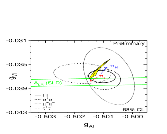
Figure 1: Contours of 68% probability in the $g^{l}_{V}-g^{l}_{A}$ plane. The solid contour results from a fit assuming lepton universality. Also shown is the one standard deviation band resulting from the $\mathrm{A}_{\mathrm{LR}}$ measurement of SLD.

3.4 Quark asymmetries

3.4.1 Heavy Flavour asymmetries

The inclusive measurement of the $b$ and $c$ asymmetries is more sensitive to $\sin^{2}\theta_{\mathrm{eff}}$ than, for instance, the leptonic forward-backward asymmetry. The reason is that $A_{b}$ and $A_{c}$ are mostly independent of $\sin^{2}\theta_{\mathrm{eff}}$, therefore $A^{b(c)}_{\mathrm{FB}}$ (which is proportional to the product $A_{e}A_{b(c)}$) is a factor 3.3(2.4) more sensitive than $A^{\mathrm{l}}_{\mathrm{FB}}$. The typical systematic uncertainty in $A^{b(c)}_{\mathrm{FB}}$ is about 0.001(0.002) and the precision of the measurement is dominated by statistics.

SLD can measure also the $b$ and $c$ left-right forward-backward asymmetry defined in equation (8) which is a direct measurement of the quark coupling $A_{b}$ and $A_{c}$. The combined fit for the LEP and SLD measurements gives

$$A^{b}_{\mathrm{FB}}=0.0990\pm 0.0021 \Longrightarrow {\sin^{2}\theta_{\mathrm{eff}}=0.23225\pm 0.00038}$$

$$A^{c}_{\mathrm{FB}}=0.0709\pm 0.0044 \Longrightarrow {\sin^{2}\theta_{\mathrm{eff}}=0.2322\pm 0.0010}$$

$$A_{b}=0.867\pm 0.035$$

$$A_{c}=0.647\pm 0.040$$

where 13% is the largest correlation between $A^{b}_{\mathrm{FB}}$ and $A^{c}_{\mathrm{FB}}$.

Taking the value of $A_{\mathrm{l}}$ given in section 3.3 and these measurements together in a combined fit gives

$$A_{b}=0.881\pm 0.018$$

$$A_{c}=0.641\pm 0.028$$

to be compared with the MSM predictions $A_{b}=0.935$ and $A_{c}=0.668$ valid over a wide range of the input parameters. The measurement of $A_{c}$ is in good agreement with expectations, while the measurement of $A_{b}$ is 3 standard deviations lower than the predicted value. This is due to three independent measurements: the SLD measurement of $A_{b}$ is low compared with the MSM, while the LEP measurement of $A^{b}_{\mathrm{FB}}$ is low and the SLD measurement of $A_{\mathrm{LR}}$ is high compared with the results of the best fit to the MSM predictions (see section 4.2).

3.4.2 Jet charge asymmetries

The average charge flow in the inclusive samples of hadronic $\mathrm{Z}$ decays is related to the forward-backward asymmetries of individual quarks:

$$\langle\mathrm{Q}_{\mathrm{FB}}\rangle = \sum_{\mathrm{q}}\delta_{\mathrm{q}}A^{\mathrm{q}}_{\mathrm{FB}}\frac{\Gamma_{\mathrm{q\bar{q}}}}{\Gamma_{\mathrm{h}}}$$ (11)

where $\delta_{\mathrm{q}}$, the charge separation, is the average charge difference between the quark and antiquark hemispheres in an event. The combined LEP value is

$${\sin^{2}\theta_{\mathrm{eff}}=0.2321\pm 0.0010}.$$

3.4.3 Comparison of the determinations of $\boldmath{\sin^{2}\theta_{\mathrm{eff}}}$

The combination of all the quark asymmetries shown in this section can be directly compared to the determination of $\sin^{2}\theta_{\mathrm{eff}}$ obtained with leptons,

$${\sin^{2}\theta_{\mathrm{eff}}=0.23222\pm 0.00033} \mathrm{(quark-asymmetries)}$$

$${\sin^{2}\theta_{\mathrm{eff}}=0.23128\pm 0.00022} \mathrm{(lepton-asymmetries)}$$

which shows a 2.4 $\sigma$ discrepancy.

Over all, the agreement is very good, and the combination of the individual determinations of $\sin^{2}\theta_{\mathrm{eff}}$ gives

$${\sin^{2}\theta_{\mathrm{eff}}=0.23157\pm 0.00018}$$

with a $\chi^{2}/\mathrm{dof}=7.8/6$ as it is shown in figure 2.

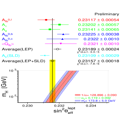
Figure 2: Comparison of several determinations of $\sin^{2}\theta_{\mathrm{eff}}$ from asymmetries.

4 Consistency with the Minimal Standard Model

The MSM predictions are computed using the programs TOPAZ0 [7] and ZFITTER [8]. They represent the state-of-the-art in the computation of radiative corrections, and incorporate recent calculations such as the QED radiator function to O($\alpha^{3}$) [9], four-loop QCD effects [10], non-factorisable QCD-EW corrections [11], and two-loop sub-leading O($\alpha^{2}\mathrm{m}^{2}_{\mathrm{t}}/\mathrm{M}^{2}_{\mathrm{Z}}$) corrections [12], resulting in a significantly reduced theoretical uncertainty compared to the work summarized in reference [13].

4.1 Are we sensitive to radiative corrections other than $\Delta\alpha$?

This is the most natural question to ask if one pretends to test the MSM as a Quantum Field Theory and to extract information on the only unknown parameter in the MSM, $\mathrm{M}_{\mathrm{H}}$.

The MSM prediction of $\mathrm{R}_{\mathrm{b}}$ neglecting radiative corrections is ${\mathrm{R}}^{0}_{\mathrm{b}}=0.2183$, while the measured value given in section 2.1 is about $2.3\sigma$ lower. From table 1 one can see that the MSM prediction depends only on $\mathrm{m}_{\mathrm{t}}$ and allows to determine indirectly its mass to be $\mathrm{m}_{\mathrm{t}}$=151$\pm$25 GeV, in agreement with the direct measurement ($\mathrm{m}_{\mathrm{t}}$=173.8$\pm$5.0 GeV).

From the measurement of the leptonic width, the vector-axial coupling given in section 3.3 disagrees with the Born prediction (-1/2) by about $3.4\sigma$, showing evidence for radiative corrections in the $\rho$ parameter, $\Delta\rho=0.0041\pm 0.0012$.

However, the most striking evidence for pure weak radiative corrections is not coming from $\mathrm{Z}$ physics, but from $\mathrm{M}_{\mathrm{W}}$ and its relation with $G_{\mu}$. The value measured at LEP and TEVATRON [14] is $\mathrm{M}_{\mathrm{W}}$=$80.39\pm 0.06$ GeV. From this measurement and through the relation

$$\mathrm{M}^{2}_{\mathrm{W}}\left(1-\frac{\mathrm{M}^{2}_{\mathrm{W}}}{\mathrm{M}^{2}_{\mathrm{Z}}}\right) = \frac{\pi\alpha}{G_{\mu}\sqrt{2}}\left(1+\Delta r\right)$$ (12)

one gets a measurement of $\Delta r=0.036\pm 0.004$, and subtracting the value of $\Delta\alpha$ ($\Delta\alpha=-\Pi_{\gamma\gamma}$), given in section 1.1, one obtains $\Delta r_{\mathrm{W}}=\Delta r-\Delta\alpha=-0.027\pm 0.004$, which is about $6.8\sigma$ different from zero. A more detailed investigation on the evidence for pure weak radiative corrections can be found in reference [15].

4.2 Fit to the MSM predictions

Having shown that there is sensitivity to pure weak corrections with the accuracy in the measurements achieved so far, one can envisage to fit the values of the unknown Higgs mass and the less well known top mass in the context of the MSM predictions. The fit is done using not only the $\mathrm{Z}$ measurements shown in this letter but also using the W mass measurements [14] and $\nu$N scattering measurements [16]. The quality of the fit is very good, ($\chi^{2}/\mathrm{dof}=13.3/14$) and the result is,

$$\mathrm{m}_{\mathrm{t}} = 161.1^{+8.2}_{-7.1}~{}\mathrm{GeV}$$

to be compared with $\mathrm{m}_{\mathrm{t}}$=173.8$\pm$5.0 GeV measured at TEVATRON. The result of the fit is shown in the $\mathrm{M}_{\mathrm{H}}$-$\mathrm{m}_{\mathrm{t}}$ plane in figure 3. Both determinations of $\mathrm{m}_{\mathrm{t}}$ have similar precision and are compatible ($1.4\sigma$). Therefore, one can constrain the previous fit with the direct measurement of $\mathrm{m}_{\mathrm{t}}$ and obtains:

$$\mathrm{m}_{\mathrm{t}}= 171.1\pm 4.9~{}\mathrm{GeV}$$

$$\log(\mathrm{M}_{\mathrm{H}}/\mathrm{GeV})= 1.88^{+0.33}_{-0.41} (\mathrm{M}_{\mathrm{H}}=76^{+85}_{-47}~{}\mathrm{GeV})$$

$$\alpha_{s}= 0.119\pm 0.003$$

with a very reasonable $\chi^{2}/\mathrm{dof}=14.9/15$. The agreement of the fit with the measurements is impressive and it is shown as a pull distribution in figure 4.

The best indirect determination of the W mass is obtained from the MSM fit when no information from the direct measurement is used,

$$\mathrm{M}_{\mathrm{W}} = 80.367\pm 0.029~{}\mathrm{GeV}.$$

The most significant correlation on the fitted parameters is 77% between $\log(\mathrm{M}_{\mathrm{H}}/\mathrm{GeV})$ and $\alpha(\mathrm{M}^{2}_{\mathrm{Z}})$. If one of the more precise new evaluations of $\Delta\alpha$ mentioned in section 1.1 is used, this correlation decreases dramatically and the precision on $\log(\mathrm{M}_{\mathrm{H}}/\mathrm{GeV})$ improves by about 30%. For instance, using $\alpha^{-1}(\mathrm{M}^{2}_{\mathrm{Z}})=128.923\pm 0.036$ from reference [2], one gets:

$$\mathrm{m}_{\mathrm{t}}= 171.4\pm 4.8~{}\mathrm{GeV}$$

$$\log(\mathrm{M}_{\mathrm{H}}/\mathrm{GeV})= 1.96^{+0.23}_{-0.26} (\mathrm{M}_{\mathrm{H}}=91^{+64}_{-41}~{}\mathrm{GeV})$$

$$\alpha_{s}= 0.119\pm 0.003$$

with the same confidence level ($\chi^{2}/\mathrm{dof}=14.9/15$) and a correlation of 39% between $\log(\mathrm{M}_{\mathrm{H}}/\mathrm{GeV})$ and $\alpha(\mathrm{M}^{2}_{\mathrm{Z}})$.

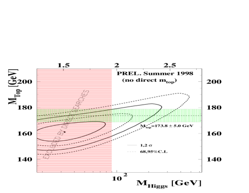
Figure 3: The 68% and 95% confidence level contours in the $\mathrm{m}_{\mathrm{t}}$ vs $\mathrm{M}_{\mathrm{H}}$ plane. The vertical band shows the 95% C.L. exclusion limit on $\mathrm{M}_{\mathrm{H}}$ from direct searches.

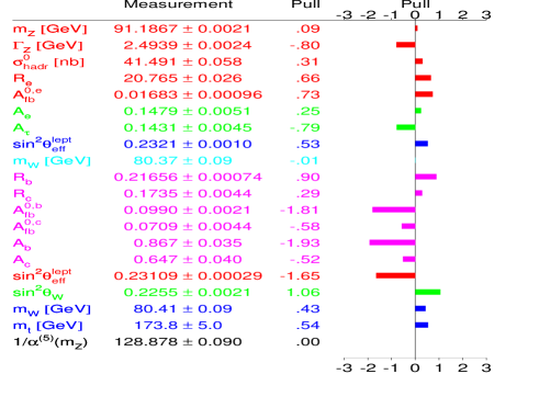
Figure 4: Pulls of the measurements with respect to the best fit results. The pull is defined as the difference of the measurement to the fit prediction divided by the measurement error.

5 Constraints on $\mathrm{M}_{\mathrm{H}}$

In the previous section it has been shown that the global MSM fit to the data gives

$$\log(\mathrm{M}_{\mathrm{H}}/\mathrm{GeV})= 1.88^{+0.33}_{-0.41} (\mathrm{M}_{\mathrm{H}}=76^{+85}_{-47}~{}\mathrm{GeV})$$

and taking into account the theoretical uncertainties (about $\pm$0.05 in $\log(\mathrm{M}_{\mathrm{H}}/\mathrm{GeV})$), this implies a one-sided 95% C.L. limit of:

$$\mathrm{M}_{\mathrm{H}} < 262~{}\mathrm{GeV}~{}@95\%~{}\mathrm{C.L.}$$

which does not take into account the limits from direct searches ($\mathrm{M}_{\mathrm{H}}>89.8~{}\mathrm{GeV}~{}@95\%~{}\mathrm{C.L.}$).

5.1 Is this low value of $\mathrm{M}_{\mathrm{H}}$ a consequence of a particular measurement?

As described in section 1.2, one can divide the measurements sensitive to the Higgs mass into three different groups: Asymmetries, Widths and the W mass. They test conceptually different components of the radiative corrections and it is interesting to check the internal consistency.

Repeating the MSM fit shown in the previous section for the three different groups of measurements with the additional constraint from [6] $\alpha_{s}=0.119\pm 0.002$ gives the results shown in the second column in table 3. All the fits are consistent with a low value of the Higgs mass, and there is no particular set of measurements that pulls $\mathrm{M}_{\mathrm{H}}$ down. This is seen with even more detail in figure 5, where the individual determinations of $\log(\mathrm{M}_{\mathrm{H}}/\mathrm{GeV})$ are shown for each measurement.

Table 3: Results on $\log(\mathrm{M}_{\mathrm{H}}/\mathrm{GeV})$ for different samples of measurements. In the fit the input parameters and their uncertainties are taken to be the values presented in section 1.1. The impact of the uncertainty in each parameter is explicitely shown.

	$\log(\mathrm{M}_{\mathrm{H}}/\mathrm{GeV})$	$[\Delta\log(\mathrm{M}_{\mathrm{H}}/\mathrm{GeV})]^{2}$	=	$[\Delta_{\mathrm{exp.}}]^{2}$	+	$[\Delta\mathrm{m}_{\mathrm{t}}]^{2}$	+	$[\Delta\alpha]^{2}$	+	$[\Delta\alpha_{s}]^{2}$
$\mathrm{Z}$ Asymmetries	$1.94^{+0.29}_{-0.31}$	$[0.29]^{2}$	=	$[0.19]^{2}$	+	$[0.12]^{2}$	+	$[0.19]^{2}$	+	$[0.01]^{2}$
$\mathrm{Z}$ Widths	$2.21^{+0.36}_{-1.43}$	$[0.36]^{2}$	=	$[0.31]^{2}$	+	$[0.14]^{2}$	+	$[0.08]^{2}$	+	$[0.13]^{2}$
$\mathrm{M}_{\mathrm{W}}$ and $\nu\mathrm{N}$	$2.04^{+0.45}_{-0.84}$	$[0.45]^{2}$	=	$[0.41]^{2}$	+	$[0.18]^{2}$	+	$[0.08]^{2}$	+	$[0.00]^{2}$

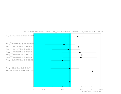
Figure 5: Individual determination of $\log(\mathrm{M}_{\mathrm{H}}/\mathrm{GeV})$ for each of the measurements.

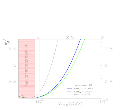
Figure 6: $\Delta\chi^{2}=\chi^{2}-\chi^{2}_{\mathrm{min}}$ vs. $\mathrm{M}_{\mathrm{H}}$ curve. Different cases are considered: the present situation, the future situation when $\Delta$$\mathrm{M}_{\mathrm{W}}$ is measured with a precision of 30 MeV and when $\Delta\alpha^{-1}=0.02$ and $\Delta$$\mathrm{m}_{\mathrm{t}}$=2 GeV. The band shows the limit from direct searches, and the discontinous line the expected limit at the end of LEP2.

5.2 Is there any chance to improve these constraints?

Although the most precise determination of the Higgs mass is still coming from the $\mathrm{Z}$ asymmetries, it is clear from table 3 that any future improvement will be limited by the uncertainty in $\alpha(\mathrm{M}^{2}_{\mathrm{Z}})$. If $\Delta\alpha^{-1}\sim 0.02$, then the error on $\log(\mathrm{M}_{\mathrm{H}}/\mathrm{GeV})$ is reduced to about 0.23 ($[\Delta_{\mathrm{exp.}}]\oplus[\Delta\mathrm{m}_{\mathrm{t}}]$), coming only from the $\mathrm{Z}$ asymmetries measurements.

The accuracy of the W-boson mass is going to improve by a significant factor in the near future. However, even if the W mass is measured with a precision of 30 MeV, the error on $\log(\mathrm{M}_{\mathrm{H}}/\mathrm{GeV})$ is going to be dominated by $\Delta\mathrm{m}_{\mathrm{t}}$ and will not be better than 0.23 obtained with the $\mathrm{Z}$ asymmetries only, both determinations being highly correlated by the uncertainty on the top mass.

Therefore, the error on $\log(\mathrm{M}_{\mathrm{H}}/\mathrm{GeV})$ is not going to improve significantly until a precise measurement of the top mass (2 GeV) becomes available. In such a case, one can easily obtain a precision in $\log(\mathrm{M}_{\mathrm{H}}/\mathrm{GeV})$ close to 0.15. This is what is shown in figure 6.

Also shown in figure 6 is the expected direct search limit from LEP2. If the tendency to prefer a very low value of $\mathrm{M}_{\mathrm{H}}$ continues with the new or updated measurements, and the accuracy on the top mass and W-boson mass are improved significantly, consistent with the indirect determinations, we may be able to constrain severely the value of $\mathrm{M}_{\mathrm{H}}$.

6 Conclusions and outlook

The measurements performed at LEP and SLC have substantially improved the precision of the tests of the MSM, at the level of O(0.1%). The effects of pure weak corrections are visible with a significance larger than three standard deviations from $\mathrm{Z}$ observables and about seven standard deviations from the W-boson mass.

The top mass predicted by the MSM fits, ($\mathrm{m}_{\mathrm{t}}$=$161.1^{+8.2}_{-7.1}$ GeV) is compatible (about $1.4\sigma$) with the direct measurement ($\mathrm{m}_{\mathrm{t}}$=$173.8\pm 5.0$ GeV) and of similar precision.

The W-boson mass predicted by the MSM fits, ($\mathrm{M}_{\mathrm{W}}=80.367\pm 0.029~{}\mathrm{GeV}$) is in very good agreement with the direct measurement ($\mathrm{M}_{\mathrm{W}}=80.39\pm 0.06~{}\mathrm{GeV}$).

The mass of the Higgs boson is predicted to be low,

$$\log(\mathrm{M}_{\mathrm{H}}/\mathrm{GeV})= 1.88^{+0.33}_{-0.41} (\mathrm{M}_{\mathrm{H}}=76^{+85}_{-47}~{}\mathrm{GeV})$$

$$\mathrm{M}_{\mathrm{H}} < 262~{}\mathrm{GeV}~{}@95\%~{}\mathrm{C.L.}$$

This uncertainty is reduced to $\Delta(\log(\mathrm{M}_{\mathrm{H}}/\mathrm{GeV}))\sim 0.23$ when the uncertainty from $\Delta\alpha$ is negligible, and will be further reduced to $\Delta(\log(\mathrm{M}_{\mathrm{H}}/\mathrm{GeV}))\sim 0.15$ when $\mathrm{m}_{\mathrm{t}}$ is known with a 2 GeV precision and $\mathrm{M}_{\mathrm{W}}$ is known with a 30 MeV precision.

References

References

-
[1]
S. Eidelman and F. Jegerlehner, Z. Phys. C 67, 585 (1995).
H. Burkhardt and B. Pietrzyk, Phys. Lett. B 356, 398 (1995). - [2] M. Davier and A. Hcker, Phys. Lett. B 419, 419 (1998).
-
[3]
J.H. Khn and M. Steinhauser, hep-ph/9802241.
M. Davier and A. Hcker, hep-ph/9805470. - [4] D. Karlen, Plenary talk at ICHEP 98, Vancouver, B.C., Canada, 23-29 July, 1998.
- [5] W. Plazcek, these proceedings.
- [6] The Particle Data Group, C. Caso et al, E. Phys. J. C 3, 1 (1998).
- [7] G. Passarino et al, hep-ph/9804211.
- [8] D. Bardin et al, hep-ph/9812201.
-
[9]
S. Jadach et al, Phys. Lett. B 257, 173 (1991).
M. Skrzypek et al, Acta Phys. Pol. B 23, 135 (1992).
G. Montagna et al, Phys. Lett. B 406, 243 (1997). -
[10]
S. Larin et al, Phys. Lett. B 400, 379 (1997).
S. Larin et al, Phys. Lett. B 405, 327 (1997).
K.G. Chetyrkin et al, Phys. Rev. Lett. 79, 2184 (1997).
K.G. Chetyrkin et al, Nucl. Phys. B 510, 61 (1998). -
[11]
A. Czarnecki et al, Phys. Rev. Lett. 77, 3955 (1996).
R. Harlander et al, Phys. Lett. B 426, 125 (1998). -
[12]
G. Degrassi et al, Phys. Lett. B 383, 219 (1996).
G. Degrassi et al, Phys. Lett. B 394, 188 (1997).
G. Degrassi et al, Phys. Lett. B 418, 209 (1997). - [13] CERN Yellow Report 95-03, Geneva, 31 March 1995, eds. D. Bardin, W. Hollik and G. Passarino.
- [14] E. Lançon these proceedings.
- [15] P. Gambino and A. Sirlin, Phys. Lett. B 73, 621 (1994).
- [16] K. MacFarland, talk presented at the XXXIIIth Rencontres de Moriond, Les Arcs, France, 15-21 March, 1998.