Available on CMS information server CMS NOTE 1998/073

November 10, 1998

Search for SUSY in (leptons +) Jets + E${}_{T}^{miss}$ Final States

S. Abdullin ^a), F. Charles ^b),

Groupe de Recherche en Physique des Hautes Energies

Université de Haute Alsace, 61 rue A.Camus 68093 Mulhouse, France

We study the observability of the strongly interacting squarks and gluinos in CMS. Classical E${}_{T}^{miss}$ + jets final state as well as a number of additional multilepton signatures (0 leptons, 1 lepton, 2 leptons of the same sign, 2 leptons of the opposite sign and 3 leptons) are investigated . The detection of these sparticles relies on the observation of an excess of events over Standard Model background expectations. The study is made in the framework of a minimal SU(5) mSUGRA model as a function of m₀, m_1/2 for 4 sets of model parameters $:$ tan$\beta$ = 2 or 35 and sign($\mu$) = $\pm$1 and for fixed value of A₀ = 0. The CMS detector response is modelled using CMSJET 4.51 fast MC code (non-GEANT). The results obtained are presented as 5 $\sigma$ detection contours in the m₀, m_1/2 planes and with optimized selection cuts in various regions of the parameter space. The result of these investigations is that with integrated luminosity L=10⁵ pb^-1 the squark and gluino mass reach is about 2.5 TeV and covers most of the interesting parts of parameter space according to neutralino relic density expectations. The influence of signal and background cross-section uncertainties on the reach contours is estimated. The effect of pile-up on signal and background is also discussed. This effect is found to be insignificant for E${}_{T}^{miss}$ and single lepton signatures, whilst only a minor deterioration is seen for multilepton final states.

^a) On leave from ITEP, Moscow, Russia. Email: adullin@mail.cern.ch
^b) Email: charles@in2p3.fr

1 Introduction

One of the main purposes of the LHC collider is to search for the physics beyond the Standard Model (SM). One of the direction of this search is a possible discovery of superpartners of ordinary particles as expected in Supersymmetric extensions of SM (SUSY). SUSY, if it exists, is expected to reveal itself at LHC via excess of (multilepton +) multijet + E${}_{T}^{miss}$ final states compared to Standard Model (SM) expectations [1].

The main goal of this study is to evaluate the potential of the CMS detector [2] to find evidence for SUSY. It deals, first with the squarks and gluino mass reach, as the production cross-section of these strongly interacting sparticles (pair production or in association with charginos and neutralinos) dominates the total SUSY cross-section over a wide region of the parameter space. In our previous study concerning maximal reach in mSUGRA for low tan$\beta$ [3] the SM background was somewhat underestimated; furthermore the signal form squarks and gluinos was taken into account, without associated production of squarks and gluino with electroweak sparticles. Besides the lepton isolation requirements at the tracker level were somewhat unrealistic (too small cone size R_isol=0.1) allowing electrons to be “isolated” in jets. Here we make a substantial revision of the results previously obtained and extend our search to the domain of large values of tan$\beta$. The effect of event pile-up on the possible mSUGRA reach is also investigated.

The paper is organized as follows. We discuss the specific SUSY model employed in section 2. In section 3 the simulation procedure issues are presented. Comparison of same signal and background distributions is shown in section 4. Section 5 describes the cuts optimization procedure allowing to adjust the cuts proposed to the condition in various domains of the model parameter space. The main results of our study are presented in section 6 where we also discuss the stability of the reach contours versus various sources of uncertainty. The conclusions are given in section 7.

2 Model employed

The large number of SUSY parameters even in the framework of Minimal extension of the SM (MSSM) makes it difficult to evaluate the general reach. So, for this study we restrict ourselves at present to the mSUGRA-MSSM model. This model evolves from MSSM, using Grand Unification Theory (GUT) assumptions (see more details in e.g. [4]). In fact, it is a representative model, especially in case of inclusive studies and reach limits expressed in terms of squark and gluino mass which do not depend critically on the specific choice of branchings and mass values as will be indirectly shown by the results of this work.

The mSUGRA model contains only five free parameters $:$

• a common gaugino mass ($m_{1/2}$) ;

• a common scalar mass ($m_{0}$);

• a common trilinear interaction amongst the scalars ($A_{0}$);

• the ratio of the vacuum expectation values of the Higgs fields that couple to $T_{3}=1/2$ and $T_{3}=-1/2$ fermions ( tan$\beta$);

• a Higgsino mixing parameter $\mu$ which enters only through its sign ($sign(\mu)$).

For a given choice of model parameters all the masses and couplings, thus production cross sections and branching ratios are fixed. At a later stage it can be generalized to the MSSM in which no such constraining relations exist.

The mass of the lightest SUSY particle (LSP) which is $\tilde{\chi}_{1}^{0}$ in the R-parity conserving mSUGRA equals approximately $\sim$ 0.5 of $\tilde{\chi}_{2}^{0}$. The mass of lightest chargino $\tilde{\chi}_{1}^{\pm}$ is almost the same as that of $\tilde{\chi}_{2}^{0}$. Isomass contours of $\tilde{\chi}_{1,2}^{0}$ and $\tilde{\chi}_{1}^{\pm}$ and gluino behave gaugino-like, i.e. depend mainly on $m_{1/2}$. Masses of sleptons and squarks depend on both $m_{0}$ and $m_{1/2}$.

Masses of squarks (especially of the first generation), gluino, charginos and neutralinos depend only weakly on tan$\beta$, A₀ or sign($\mu$) parameters. Masses of sleptons, stop and sbottom have some dependence on these mSUGRA parameters, whilst masses of Higgs bosons depend significantly on tan$\beta$ (see some examples e.g. in [5]), the mass of lightest scalar Higgs increases with tan$\beta$ and depends also on sign($\mu$), whilst masses of the heavy Higgses decreases dramatically with tan$\beta$.

Since masses, branchings, cross-sections vary most rapidly with m₀, m_1/2, it is natural to follow the commonly used way of presenting mSUGRA data as a function of these two parameters for different fixed values of tan$\beta$ and sign$(\mu$). The A₀ parameter is usually set to zero, since its variation has small effect on the results. Figs.1,2 show isomass contours of SUSY particles for some particular choice of mSUGRA parameters, namely $:$ tan$\beta$ = 2, A₀ = 0 and $\mu$ $<$ 0 just to have some idea about the characteristic values and behaviour of the masses versus m₀ and m_1/2. The shaded regions along the axes denotes theoretically (TH) and up to now experimentally (EX) excluded regions of the model parameter space. The data concerning these regions were taken from [6] .

The MSSM establishes the relation between the top mass and tan$\beta$ (see e.g. [7]) $:$

m${}^{2}_{t}$ = 4$\pi$Y${}_{t}v^{2}$ $\frac{tan^{2}\beta}{1+tan^{2}\beta}$                                    (1)

Here Y_t is top Yukava coupling. For low tan$\beta$ the top Yukava coupling can be derived from known gauge couplings alone, which leads to the tan$\beta$ value of 1.6$\pm$0.3 for m_t = 175$\pm$6 GeV. Taking into account behaviour of bottom and $\tau$ Yukava couplings at large tan$\beta$ (see discussion e.g. in [5]), it seems to be possible to find second solution of eq.(1) with tan$\beta$ $\approx$ 33$\pm$3 (see also Fig.6 in [7]). So, from now on we will consider mainly dependence of various mSUGRA observables and will present our results for 4 sets of tan$\beta$ and $\mu$ parameters, keeping A₀=0, see Table.1.

Figure 1: Isomass contours of squarks($\tilde{q}$), gluino($\tilde{g}$), lightest scalar(h) and pseudoscalar(A) Higgs fields as a function of mSUGRA parameters m0, m1/2 for fixed values of tan$\beta$=2, $\mu$$<$0 and A0=0. Numbers in parenthesis denote the masses in GeV.		Figure 2: Isomass contours of left($\tilde{l}_{L}$) and right($\tilde{l}_{R}$) sleptons and next-to-lightest neutralino($\tilde{\chi}_{2}^{0}$) with the same choise of mSUGRA parameters as in Fig.1. Note expanded scale compared to Fig.1.

Table 1: Sets of mSUGRA parameter values investigated.

mSUGRA parameter
Set	tan$\beta$	sign($\mu$)
1	2	-1
2	2	+1
3	35	-1
4	35	+1

Figure 3: Total mSUGRA cross-section contours as a function of m0, m1/2 for mSUGRA Set 1 (solid line). The contribution of $\tilde{g}\tilde{g}$, $\tilde{g}\tilde{q}$, $\tilde{q}\tilde{q}$ production alone is shown by dashed line.		Figure 4: Same as Fig.3, except for Set 2.

Figure 5: Same as Fig.3, except for Set 3.		Figure 6: Same as Fig.3, except for Set 4.

In Figs.3-6 one can see total mSUGRA production cross-section as a function of m₀, m_1/2 for chosen sets of tan$\beta$ and sign($\mu$). The contribution of strongly interacting SUSY particles cross-section is also shown by dashed line. The jitter of contours is caused by limited statistics. The total cross-section for different values of tan$\beta$ and sign($\mu$), but for the same values of m₀, m_1/2 differs slightly. The bulk of the total cross-section for low values of m_1/2 consists from $\tilde{g}\tilde{g}$, $\tilde{g}\tilde{q}$, $\tilde{q}\tilde{q}$, whereas in the domains with extremely high masses of $\tilde{g}$, $\tilde{q}$ the contribution of production of squarks or gluinos associated with charginos and neutralinos may dominate.

Figs.7 and 8 shows the typical decay modes of heavy gluino and left squark in case of high tan$\beta$, when $\tilde{\chi}_{2}^{0}$ and $\tilde{\chi}_{1}^{\pm}$ branching ratios for decays into $\tilde{\tau}_{1,2}$ $\tau(\nu)$ exceed 60 $\%$ due to large tau Yukava couplings [5]. To simplify the figure, similar intermediate final states were joined. For instance, states $\tilde{\chi}_{2}^{\pm}$Wbb and $\tilde{\chi}_{2}^{\pm}$tb were treated(summed up) as the same, though they have different kinematics, in principle (see the rightmost round mark at $\tilde{\chi}_{2}^{\pm}$ horizontal line (1067 GeV). It is almost impossible to follow and calculate all the branchings for gluino decays, so some small ones are not shown thus resulting in some small underestimate of the “final” states (at the level of $\tilde{\chi}_{1}^{0}$) branching ratios. The final states having the highest branching ratios are listed in the lower part of Figs.7 and 8. The right squarks ($\tilde{q}_{R}$) decay entirely into $\tilde{\chi}_{1}^{0}$ q final state in the domain of mSUGRA parameter space where m${}_{\tilde{q}_{R}}<$m${}_{\tilde{g}}$ as it is in the point presented in Figs.7 and 8. Decay chains of $\tilde{b}_{1,2}$ or $\tilde{t}_{1,2}$ are somewhat intermediate between those for $\tilde{q}_{L}$ and $\tilde{g}$ from the point of view of variety of final states.

Figs.9 and 10 show typical decay modes of a heavy gluino and left squark respectively, at the same point of parameter space as in Figs.7 and 8, except for low tan$\beta$=2. Right squarks again decay entirely into LSP + quarks. One can see that decay chains of gluino are not so complicated in case of low tan$\beta$, mainly due to the fact that m${}_{\tilde{t}_{1}}<$m${}_{\tilde{\chi}_{2}^{\pm},\tilde{\chi}_{3,4}^{0}}$. In addition, at low tan$\beta$ $\tilde{\tau}_{1,2}$ do not dominate in the decays of $\tilde{\chi}_{1}^{\pm}$ and $\tilde{\chi}_{2}^{0}$, instead, branchings of $\tilde{\chi}_{1}^{\pm}$ and $\tilde{\chi}_{2}^{0}$ decays into sleptons are enhanced. So final states of left squarks and gluino contain more leptons in case of low tan$\beta$ than in case of high tan$\beta$ in the chosen particular point of mSUGRA parameter space. The latter statement is more general, namely this difference in the yield of leptons between low and high tan$\beta$ exists in significant domains of m₀, m_1/2 values along the theoretically excluded region at low values of m₀, where $\tilde{\chi}_{1}^{\pm}$ and $\tilde{\chi}_{2}^{0}$ have 2-body decays.

Figure 7: Typical decay modes for massive (2060 GeV) gluino for high tan$\beta$ ( m₀=400 GeV, m_1/2=900 GeV, Set 4).

Figure 8: Same as Fig.7, but for first generation left squarks (1857 GeV)

Figure 9: Typical decay modes for massive (2082 GeV) gluino for low tan$\beta$ ( m₀=400 GeV, m_1/2=900 GeV, Set 2).

Figure 10: Same as Fig.9, but for first generation left squarks (1867 GeV)

Figure 11: Probability to find at least one lepton in the final state (e or $\mu$ as defined in text) in signal evens as a function of m0, m1/2 for mSUGRA Set 1.		Figure 12: Same as Fig.11, except for Set 2.

Figure 13: Same as Fig.11, except for Set 3.		Figure 14: Same as Fig.11, except for Set 4.

Figs.11-14 illustrate the fact that mSUGRA final states frequently contain lepton(s). The plots show the probability to find at least one lepton per mSUGRA event above some p_T threshold (10 GeV for muons, 20 GeV for electrons) within the detector acceptance ( $|\eta|<$ 2.4). The source of these leptons are mainly b-jets produced in the decay chains of sparticles, then W and Z-bosons produced both in decays of top and chargino/neutralino decays. One of the abundant sources of leptons in mSUGRA final states are also leptonic decays (2-body via sleptons or direct 3-body) of charginos and neutralinos (mainly $\tilde{\chi}_{2}^{0}$, $\tilde{\chi}_{1}^{\pm}$) in some domains of the parameter space. One can see the domain where $\tilde{\chi}_{2}^{0}$, $\tilde{\chi}_{1}^{\pm}$ have significant branching ratio for the decays into sleptons $\rightarrow$ leptons on the right side of Figs.11 and 12 (small m₀ values). A similar situation, but not so pronounced can be seen in Figs.13 and 14, where the spike in the vicinity of m₀=600 GeV, m_1/2=1500 GeV reflects the increased (with increase of m_1/2) branchings of $\tilde{\chi}_{2}^{0}$, $\tilde{\chi}_{1}^{\pm}$ into $\mu$,e-sleptons, thus replacing high branchings of $\tilde{\chi}_{2}^{0}$, $\tilde{\chi}_{1}^{\pm}$ into $\tilde{\tau}_{1,2}$ at low values of m₀, m_1/2. In the mentioned extreme point with m₀=600 GeV, m_1/2=1500 GeV we have Br($\tilde{\chi}_{2}^{0}$ $\rightarrow$ $\tilde{\chi}_{1}^{0}$ $l^{+}l^{-}$) = 23 % and Br($\tilde{\chi}_{1}^{\pm}$ $\rightarrow$ $\tilde{\chi}_{1}^{0}$ $l^{\pm}\nu$) = 42 %.

All the figures showed in this section are drawn using calculations made with ISAJET 7.32 generator [8] and supplements therein. One can also take a look at the relevant figures of mSUGRA events in CMS detector selected and reconstructed with fast MC code called CMSJET [9] used in this study (see also section 3) and then drawn with CMSIM [10] GEANT-based CMS detector simulation package. Figs.2 and 10 in [11] are $\tilde{g}$, $\tilde{q}$ events with different final states in two distant points in mSUGRA parameter space. We do not show them here because of the extremely large size of these drawings (some 12 Mb).

3 Simulation procedure

The PYTHIA 5.7 generator [12] is used to generate all SM background processes, whereas ISAJET 7.32 is used for mSUGRA signal simulations. The CMSJET (version 4.51) fast MC package [9] is used to model the CMS detector [2] response, since it still looks impossible to perform a full-GEANT simulation for the present study, requiring to process multi-million samples of signal and SM background events. A sketch of the calorimeter model implemented in CMSJET is shown in Fig.15. The sign “+” in the $\sigma$/E expressions means sum in quadrature everywhere it appears in this figure.

The SM background processes considered are $:$ QCD 2 $\rightarrow$ 2 (including $b\bar{b}$), $t\bar{t}$, $W+jets$, $Z+jets$. The $\hat{p}_{T}$ range of all the background processes is subdivided into several intervals to facilitate accumulation of statistics in the high-$\hat{p}_{T}$ range $:$ 100-200 GeV, 200-400 GeV, 400-800 GeV and $>$ 800 GeV (additional interval of 800-1200 GeV is reserved for QCD). The accumulated SM background statistics for all background channels is presented in Tab.2, whilst the signal data samples are given in Tab.3.

The grid of probed m₀, m_1/2 mSUGRA points has a cell size of $\Delta$m₀=$\Delta$m_1/2=100 GeV for m${}_{0}<$1000 GeV and $\Delta$m₀=200 GeV, $\Delta$m_1/2=100 GeV for m${}_{0}>$1000 GeV. Set 4 was also probed with the appropriate mixture of signal and pile-up events (see details in subsection 6.4).

Table 2: SM background statistics generated.

Bkgd channel	$\hat{P}_{T}$ interval	$\sigma$ (pb)	Nev generated	% of needed
	(GeV)	(pb)		for 100 fb-1
	0 - 100	267	1.461$\cdot$107	54.7
	100 - 200	240	6.638$\cdot$106	27.7
$t\bar{t}$	200 - 400	80.7	6.864$\cdot$106	85.1
	400 - 800	6.3	6.484$\cdot$105	102.9
	$>$ 800	0.163	1.630$\cdot$104	100.0
	50 - 100	2670	1.554$\cdot$107	5.8
	100 - 200	580	9.998$\cdot$106	17.2
$Zj$	200 - 400	64.0	4.455$\cdot$106	71.2
	400 - 800	4.0	4.927$\cdot$105	123.2
	$>$ 800	0.137	1.370$\cdot$104	100.0
	50 - 100	7140	2.753$\cdot$107	3.9
	100 - 200	1470	8.618$\cdot$106	5.9
$Wj$	200 - 400	155	6.424$\cdot$106	41.4
	400 - 800	9.5	9.909$\cdot$105	104.3
	$>$ 800	0.33	3.300$\cdot$104	100.0
	100 - 200	1.37$\cdot$106	6.000$\cdot$107	0.04
	200 - 400	7.15$\cdot$104	3.229$\cdot$107	0.45
$QCD$	400 - 800	2740	3.259$\cdot$107	11.9
(incl. $b\bar{b}$)	800 - 1200	60.0	6.033$\cdot$106	100.5
	$>$ 1200	4.8	4.947$\cdot$105	103.1
total			2.342$\cdot$108

Table 3: mSUGRA signal statistics generated.

Set No.	No. of probed m0, m1/2 points	Total statistics generated
1	120	1.95$\cdot$106
2	114	1.87$\cdot$106
3	99	0.68$\cdot$106
4	100	0.75$\cdot$106
4 with pile-up	67	0.18$\cdot$105
total	500	5.43$\cdot$106

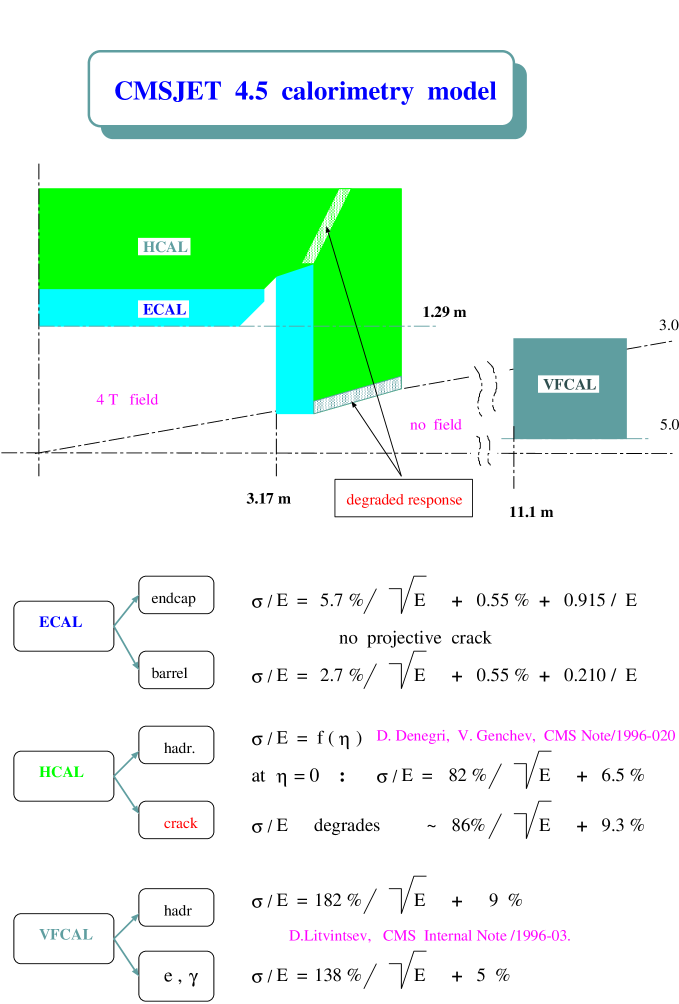
Figure 15: Sketch of calorimetry description in CMSJET.

It is very difficult to produce a representative sample of QCD jet background in the low-$\hat{p}_{T}$ range since the cross section is huge and we need extreme kinematical fluctuations of this type of background to be within the signal selection cuts. Even having spent a couple of CPU years and using fast MC we are able to exploit only a tiny fraction of QCD background of low-$\hat{p}_{T}$ values. Fortunately, there is a correlation between $\hat{p}_{T}$ and maximal produced E${}_{T}^{miss}$ value, since the main sources of E${}_{T}^{miss}$ in QCD events, such as neutrinos form b,c-jets and E${}_{T}^{jet}$ mis-measurement, strongly correlate with the $\hat{p}_{T}$. This allows one not to expect high values of E${}_{T}^{miss}$ from low-$\hat{p}_{T}$ QCD events.

Nevertheless, to be on the safe side, we cannot go confidently below $\simeq$ 200 GeV with the cut on E${}_{T}^{miss}$, where the QCD jet background becomes the dominant contribution and where our simulations are not yet fully reliable for this type of background, as it depends on the still evolving estimates of dead areas/volumes due to services etc.

Initial requirements for all the samples are the following $:$

• at least 2 jets with E${}_{T}^{jet}$ $>$ 40 GeV in $\mid\eta^{jet}\mid$ $<$ 3

• E${}_{T}^{miss}$ $>$ 200 GeV

In this analysis in general no specific requirements are put on leptons. If there are isolated muons with p${}_{T}^{\mu}$ $>$ 10 GeV within the muon acceptance, or isolated electron with p${}_{T}^{e}$ $>$ 20 GeV within $\mid\eta^{e}\mid$ $<$ 2.4 in the event, they are also recorded to use them in the subsequent analysis. The term “isolated lepton” here means satisfying simultaneously the following two requirements $:$

• no charged particle with p_T $>$ 2 GeV in a cone R = 0.3 around the direction of the lepton,

• $\Sigma$ E${}_{T}^{cell}$ in a “cone ring” 0.05 $<$ R $<$ 0.3 around the lepton impact point has to be less than 10 % of the lepton transverse energy

The electrons are always required to satisfy these isolation criteria due to identification requirements, whilst muons can be identified even in jets, so isolation is not mandatory to identify them. Hence muon isolation requirement can be used to optimize the results. A factor of “detection efficiency” of $\epsilon$=0.9 is applied for each lepton to take into account various inefficiencies of the full pattern recognition.

4 mSUGRA signal and “SM background”

In the following the term mSUGRA signal means the sum of all sparticle production processes $:$ $\tilde{g}$, $\tilde{q}$ pair and associated with other sparticles (e.g. $\tilde{\chi}_{2}^{0}$ and $\tilde{\chi}_{1}^{\pm}$), chargino-neutralino pair production etc. The SM background includes processes listed in Tab.2. All the specific signal final states investigated here mean samples of events from the total mSUGRA signal passing initial requirements listed in section 3 and classified according to presence (or total absence) of a definite number of isolated electrons and (isolated or not) muons in the final state. The E${}_{T}^{miss}$ signature means that the whole signal sample satisfies requirements concerning jets and E${}_{T}^{miss}$ beyond initial ones, and is treated without taking into account possibly identified leptons. The 0l signature implies a lepton veto with the leptonic requirements listed in section 3.

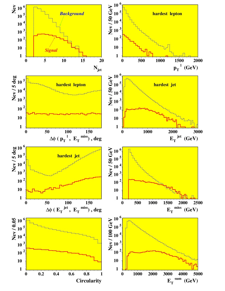
Figure 16: Comparison of the mSUGRA signal and SM background, with 100 fb^-1, in one point of mSUGRA parameter space $:$ m₀=1000 GeV, m_1/2=800 GeV, Set 4. (m${}_{\tilde{g}}$$\approx$m${}_{\tilde{q}_{L}}$$\approx$ 1900 GeV) for the E${}_{T}^{miss}$ signature. Initial cuts are applied.

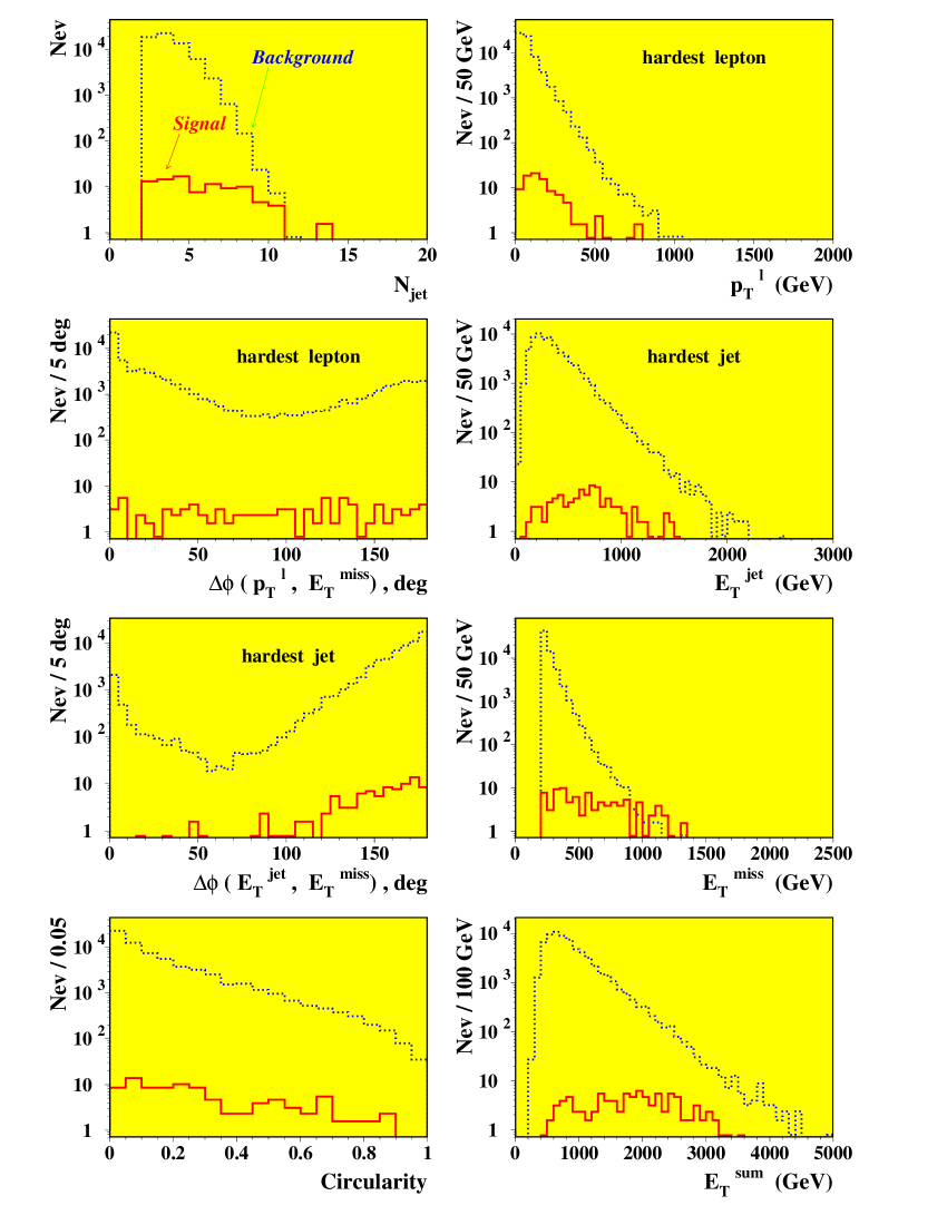
Figure 17: Same as Fig.16, except for 2l OS final states.

The 1l signature means presence of a single lepton found in the event, 2l SS - two leptons of same sign, 2l OS - two leptons of opposite sign and 3l - three leptons in the event with leptons satisfying the basic criteria specified in section 3, and there are the basic E${}_{T}^{miss}$ and jets requirements.

The kinematics of signal events is usually harder than that of SM background for the interesting regions of maximal reach of squark-gluino masses . The cross-section of the background is however higher by orders of magnitude and high-p_T tails of different backgrounds can have a kinematics similar to that of the signal.

In Fig.16 we compare some signal distributions for the point (m₀, m_1/2) = (1000,800) of Set 4, corresponding to m${}_{\tilde{g}}\approx$ m${}_{\tilde{q}_{L}}\approx$ 1900 GeV, m${}_{\tilde{\chi}_{1}^{0}}$ = 351 GeV, m${}_{\tilde{\chi}_{2}^{0}}$ = m${}_{\tilde{\chi}_{1}^{\pm}}$ = 668 GeV, and distributions of the sum of all SM background processes listed in Tab. 2 for the E${}_{T}^{miss}$ signature. Both signal and background histograms contain only events satisfying first level selection criteria. Only the hardest jet and lepton in the event are shown in distributions in Fig.16.

Fig.17 shows the same comparison at the same mSUGRA point as in Fig.16, except for the 2l OS final state signature, with non-isolated muons. Both the signal and background samples are significantly smaller than those in Fig.16 (with the same initial cuts).

Since the topology of signal and background events is rather similar already after first level selection cuts, the difference in the angular distributions and circularity is not significant either, it is thus not very useful to apply cuts on these variables too. The difference in the lepton p_T distributions is also not very pronounced as signal leptons are produced in cascade decays, thus loosing “memory” about the hardness of the original process. But for extremely high masses of squarks or gluinos ($\sim$ 2 TeV), there is some difference in the angular and p${}_{T}^{l}$ distributions between signal and the total SM background. For example, the W+jets background contributes significantly in the leftmost part of the $\Delta\phi(p_{T}^{l},E_{T}^{miss})$ distribution, especially in case of the 1l signature with high cuts on E${}_{T}^{miss}$ and jets E${}_{T}^{j}$. So cuts on these variables can be useful in these conditions.

One can deduce from Figs.16 and 17 that cuts on the jet multiplicity N_j and E${}_{T}^{miss}$ are the most profitable ones for background suppression . Of course, there is inevitable correlation between variables both in signal and background, e.g. an obvious correlation between E${}_{T}^{miss}$ and the hardest jet E_T in QCD events, since there E${}_{T}^{miss}$ is mainly produced by neutrinos from b-jets and/or high-E${}_{T}^{jet}$ mis-measurement. This can lead to a degradation of the efficiency of some cuts, if fixed cuts are used. It is thus more profitable to have adjustable cuts to meet various kinematical conditions in various domains of mSUGRA parameter space and take into account difference in topology between various signatures.

Anyway, the cuts have to be justified from the point of view of the best observability of the signal over expected background, and in all cases, signal observability is based on an excess of events of a given topology over known (expected) backgrounds.

5 Cuts optimization procedure

5.1 General considerations

The chosen criterion of the mSUGRA signal observability is S $\geq$ 5 $\cdot$ $\sqrt{S+B}$, where S means number of mSUGRA signal events, B - number of SM background. In other words, it can be expressed as signal (= all recorded - SM expectations) has to be five times larger than the square root of all events kept. So cuts have to be adjusted in each probed mSUGRA point in such a way that the observability function S / $\sqrt{S+B}$ be maximal.

The set of cuts on selected variables applied in each probed point to both signal and background to find the best observability is shown in Table 4. The total number of combinations exceeds 10⁴, but in practice, only part of the entire “cut space” (1000 - 3000 combinations) is really used to optimize the reach for each topology and for each mSUGRA parameter Set. The procedure works as follows. All the cut combinations are applied independently at each probed point of parameter space as well as to the background samples. The best value of the observability function is then evaluated in each point, having summed data over all background channels for each particular cut combination. The smooth boundary curve is then found interpolating between m₀ and m_1/2 points.

Table 4: Sets of cuts.

Variable(s)	Values	Total number
Nj	2, 3, 4, …, 10	9
E${}_{T}^{miss}$	200, 300, 400, …, 1400 GeV	14
E${}_{T}^{j1}$	40, 150, 300, 400, 500, 600, 700, 800, 900, 1000 GeV	10
E${}_{T}^{j2}$	40,  80, 200, 200, 300, 300, 400, 400, 500,  500 GeV
$\Delta\phi$ $(p_{T}^{l},E_{T}^{miss})$	0, 20 deg.	2
$Circularity$	0,  0.2	2
$\mu$ isolation	on, off	2
total		$\approx$ 104

5.2 Numerical examples

Just to give an idea about orders of magnitude, we show in Table.5 some numerical examples of best cuts found in a few representative points of Set 4. The points are chosen near the 5 $\sigma$ reach boundary for the corresponding experimental final state signature.

Table 5: Numerical examples of cuts optimization with integrated luminosity of 100 fb^-1.

	Point of Set 4		Cuts values						S	B (ev)
Signature	m0	m1/2	Nj	E${}_{T}^{miss}$	E${}_{T}^{j1}$, E${}_{T}^{j2}$	$\Delta\phi$	$Circ.$	$\mu$-isol.	(ev)	$t\bar{t}$	$Wj$	$Zj$	$QCD$	All	$\frac{S}{\sqrt{S+B}}$
	(GeV)	(GeV)		(GeV)	(GeV)	(deg)		(on/off)
E${}_{T}^{miss}$	500	1200	2	1200	900, 600	0	0	off	57.0	4	18	17.6	1	40.6	5.77
	1600	1000	7	600	600, 300	0	0	off	27.6	1	2	3.8	8.8	15.6	4.2
1l	400	1100	2	900	600, 300	20	0	on	31.9	1.8	13.2	0	0	15.0	4.66
	1000	1000	4	800	500, 300	20	0	off	36.0	4.5	11.5	7.1	0	23.1	4.68
3l	400	700	2	300	150, 80	0	0	on	41.3	0	0.7	0	0	0.7	6.37
	1400	700	2	300	300, 200	0	0	off	37.7	8	2.5	15.8	0	26.3	4.72

6 Results

6.1 5 $\sigma$ reach

Figs.18-21 show the main results of our study for mSUGRA parameter sets given in Tab.1 assuming an integrated luminosity of 100 fb^-1. Fig.22 regroups Figs.18-21 together, without details, just for visual comparison of respective searches. The dashed-dotted lines in Figs.18-21 are isomass contours for squarks ($\tilde{q}$), gluino ($\tilde{g}$) and lightest scalar Higgs ($h$). Numbers in parenthesis denote mass values of corresponding isomass contour. The neutralino relic density contours from ref. [6], for mSUGRA domain m₀$<$1000 GeV, m_1/2$<$1000 GeV, are also shown in Figs.18-21 for $\Omega h^{2}$ = 0.15, 0.4 and 1.0. Value $\Omega h^{2}$$>$1 would lead to a Universe age less than 10 billion years old, in contradiction with estimated age of the oldest stars. The region in between 0.15 and 0.4 is favoured by the Mixed Dark Matter (MDM) cosmological models.

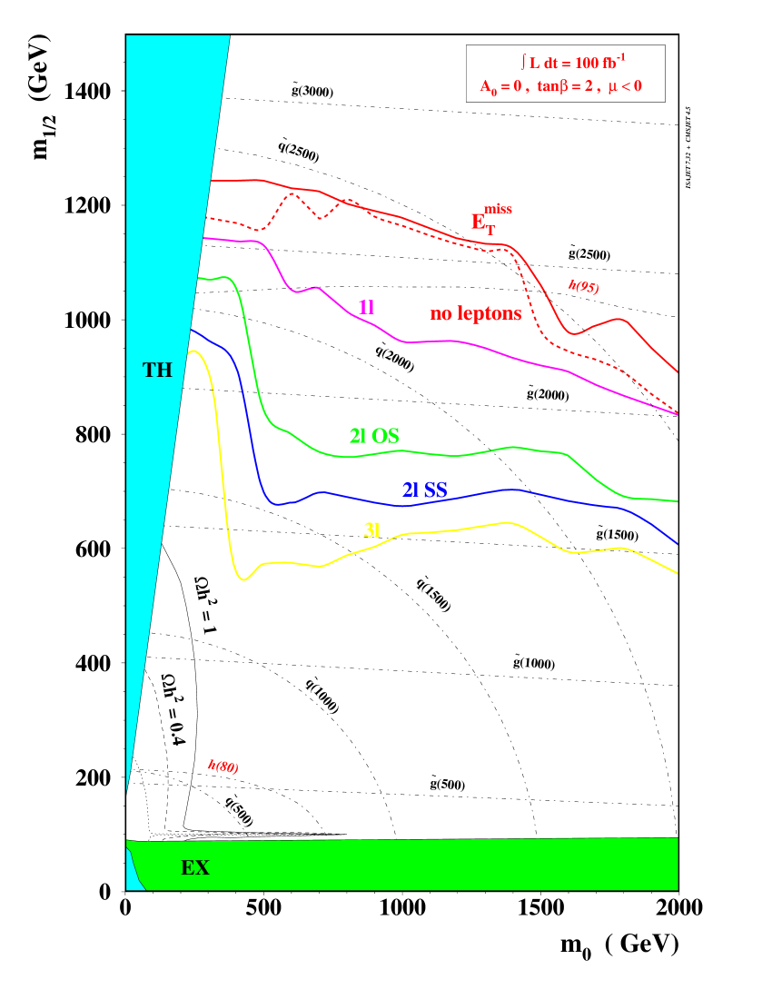
Figure 18: 5 sigma reach contours for various final states with 100 fb^-1 for Set 1 (see also comments in text).

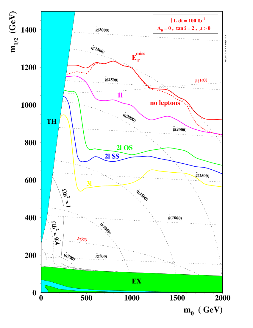
Figure 19: Same as Fig.18, but for Set 2.

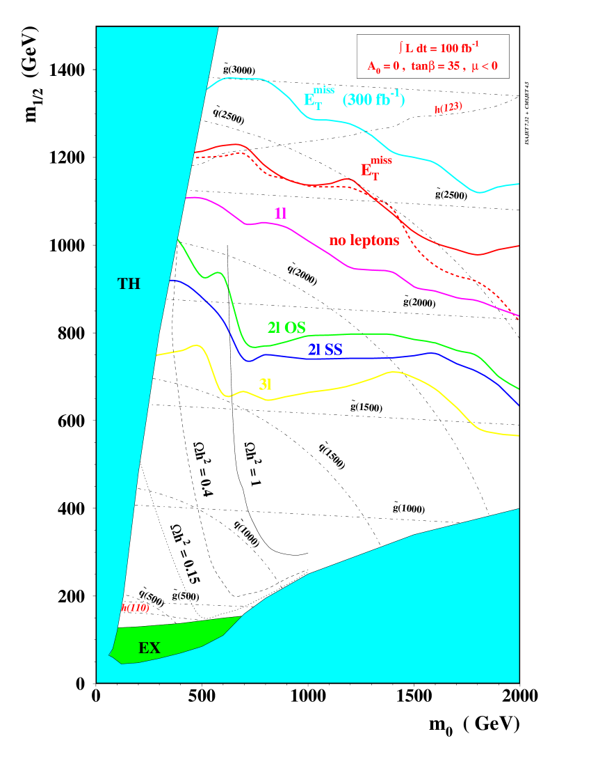
Figure 20: Same as Fig.18, but for Set 3.

Figure 21: Same as Fig.18, but for Set 4.

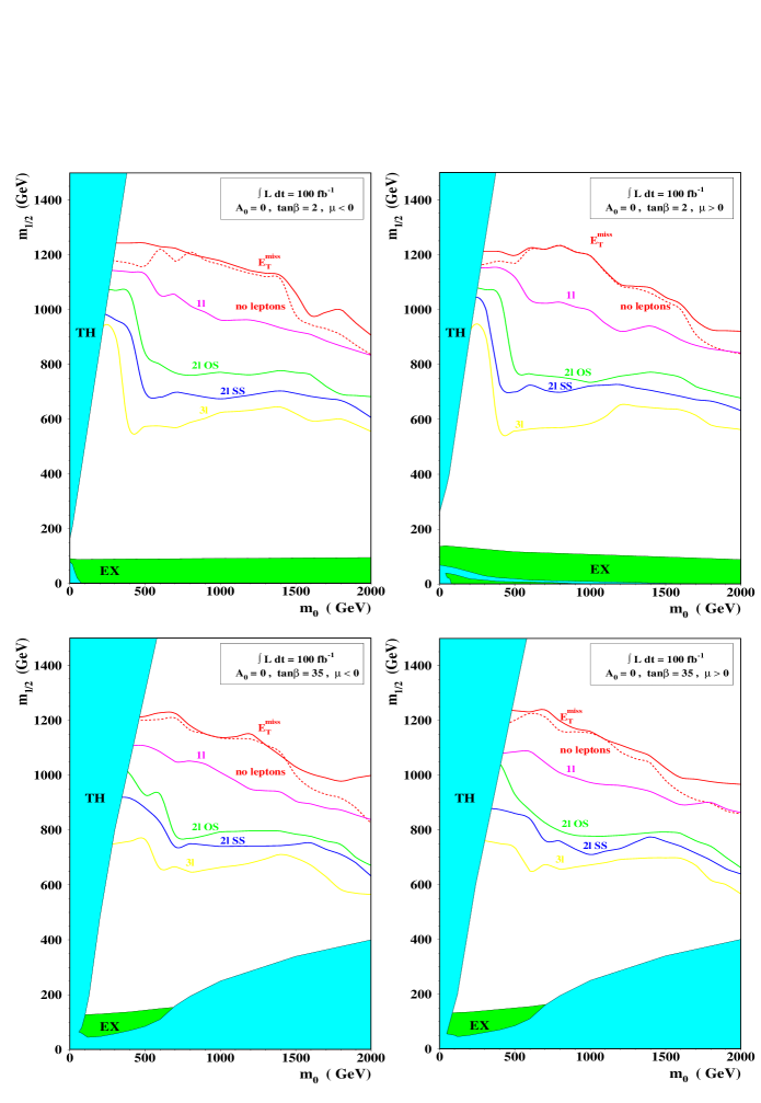
Figure 22: Simplified Figs.18-21 put together.

It is a rather general situation that for all investigated sets of mSUGRA parameters the best reach can be obtained with the E${}_{T}^{miss}$ signature. The more leptons required - the smaller reach, as can be seen from Figs.18-22. For Set 1 one can see that the entire m₀, m_1/2 plane (Fig.18) is covered, in principle by LEP II through Higgs searches. This is not the case for Set 2 (Fig.19). Anyway, for low tan$\beta$ cosmologically interesting regions will be definitely covered by LEP II or LHC reach. I does not seem so evident for high values of tan$\beta$ (Figs.20 and 21), where the calculations of $\Omega h^{2}$=1 contours available are limited to m_1/2 $\leq$ 1000 GeV. But again, the cosmologically preferred region $\Omega h^{2}$$<$0.4 seems to be entirely within the reach of CMS. In both Figs.20 and 21 we also show our calculations for the E${}_{T}^{miss}$ signature reach for an integrated luminosity of 300 fb^-1, trying to estimate the ultimate CMS reach. The Higgs contours in Figs.20 and 21 show that most of the m₀, m_1/2 planes is out of reach for LEP II.

It is worth noticing that the cumulative reach of several signatures, like 0l + 1l + 2l + 3l + … (in descending order of contribution) can be even better than the most promising single E${}_{T}^{miss}$ signature. We show this with the cumulative 0l + 1l + 2l OS signatures curve (main leptonic signatures) in Fig.21. Despite the fact that this curve does is not obtained with the optimally adjusted cuts (each signature was optimized separately to have the best significance and then signal and background values were summed up for all three signatures), one can see that the reach obtained is better than that of the E${}_{T}^{miss}$ signature.

Here we do not consider the limitations on the mSUGRA parameter space imposed by the $b$ $\rightarrow$ $s\gamma$ calculations [13] based on the data from CLEO [14]. These calculations exclude at 95 % CL the part of m₀, m_1/2 plane approximately below squark isomass contour of 1600 GeV for Set 3 and below a similar contour of $\approx$ 600 GeV for Set 4 respectively. For low tan$\beta$ (Sets 1 and 2) the mSUGRA parameter space domain excluded this way is rather small [15].

6.2 Effect of the muon isolation requirement on the reach

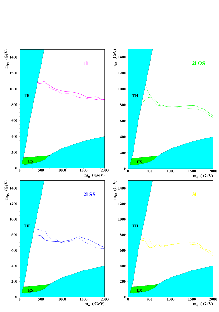
Figure 23: Effects of the muon isolation requirement on the 5$\sigma$ contours for Set 4. The reach without a muon isolation requirement is shown by a solid line, the dashed line denotes the reach with the muon isolation requirement applied.

In our study we always require that the isolation criterion mentioned in section 3 be fulfilled by electrons, so as to be identified in the CMS detector. On the contrary the muon isolation requirement is a parameter in the cuts optimization procedure described in section 5. This is so as a muon can be identified even when it is embedded in a jet. Fig.23 illustrates the effect of the muon isolation requirement on the reach contours for various multilepton signatures for mSUGRA parameter Set 4 with 100 fb^-1. One can see that for low values of m₀ it is profitable to apply muon isolation (dashed line), whilst for high m₀ values some small gain can be obtained by not applying the muon isolation criterion (solid line). This is due to some difference in the origin of leptons in these two domains of m₀. As it was discussed in section 2 ( can also be seen in Figs.7 and 8), the sources of isolated leptons in the low-m₀ region of Set 4 are mainly $\tau$ and W abundantly produced in the cascade decays of squarks and gluinos. In the high-m₀ region of Set 4 the situation changes slightly $:$ W-bosons are still present in cascades of strongly interacting sparticles, but increasing average number of b-jets (e.g. $\tilde{\chi}_{2}^{0}$ almost completely decay into $\tilde{\chi}_{1}^{0}h$, and Higgs in turn has branching into $b\bar{b}$ of $\approx$ 80-90 %) contributes significantly to the increase of non-isolated muon production.

6.3 Stability of results versus variations of signal and background cross sections

As can be seen from the numerical examples shown in Tab.5, in the vicinity of 5 $\sigma$ reach boundary the S/B ratio is generally $>$ 1. So one can expect that the stability of the 5 $\sigma$ reach in terms of S / $\sqrt{S+B}$ depends largely on the variations of the signal rather than on the background. We are aware however that PYTHIA can underestimate the W/Z + jets cross section, especially for multijet events. Fig.24 shows the band of the 5 $\sigma$ reach for E${}_{T}^{miss}$ and 2l SS signatures for Set 4 induced by varying the mSUGRA signal cross section within $\pm$ 30 % around the nominal value given by ISAJET. In Fig.25 one can see the uncertainty band similar to that in Fig.24, but now the SM background cross section is varied by a factor of 2. The width of the band for the 2l SS signature in Fig.25 is rather small and is of the order of pure statistical uncertainties.

6.4 Effect of event pile-up on the results

Adding event pile-up to the SM background at the generation stage causes a few times larger CPU consumption by the CMSJET package than without pile-up, since the number of fired cells (crystals, towers) to be processed increases significantly. Besides, in the frame of the mentioned package, only a limited sample of pile-up events (10³-10⁴ bunch crossings) can be used as an external input file due to the large scale (hundreds of Mb) of pile-up hits file (similar to that of CMSIM one). The limited size of pile-up sample means inevitably some bias in the data. These are the two main reasons why the SM background files were produced without pile-up admixture.

Figure 24: The band of variation of the reach contour for E${}_{T}^{miss}$ and 2l SS signatures with 100 fb-1 for a $\pm$ 30 % variation of mSUGRA cross-sections for Set 4. The upper band edge corresponds to an increase of the mSUGRA cross section by 30 %, the lower one - to the same decrease.		Figure 25: Same as Fig.24, except for variation of SM cross-sections by a factor of 2. The upper band edge corresponds to SM cross-sections decreased by a factor of 2, the lower one - to the same increase.

It is evident that in heavy event pile-up conditions one can expect some changes in both kinematical distributions (increase of the mean jet number, degradation of E${}_{T}^{miss}$ resolution etc.) and deterioration of the lepton isolation. To estimate the effect of pile-up on the signal and background distributions, we compare some of the main distributions with in the presence of pile-up and without it. Pile-up is taken from PYTHIA’s MSEL=2 with the $<$25$>$ interactions per bunch crossing.

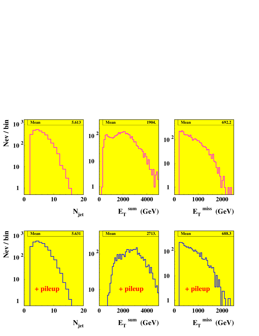
Figure 26: Effect of event pile-up on the mSUGRA distributions at one point of parameter space $:$ m₀=1000 GeV, m_1/2=800 GeV for Set 4 (same point as in Figs.15,16).

Figure 27: Effect of event pile-up on some QCD distributions (400$<\hat{p}_{T}<$800 GeV). The upper row of figures is produced without pile-up, the lower ones - with pile-up added.

Fig.26 shows the effect of pile-up on distributions on the number of jets, the summed E_T flow through detector and the E${}_{T}^{miss}$ at some representative point of parameter space. One can see a rather insignificant effect of pile-up on the distributions presented, except for the increase of the transverse energy by $\approx$ 800 GeV, this is just the quantitative characteristic of the pile-up itself, the same increase is expected for any kind of events. Fig.27 shows effects of pile-up on the same distributions as in Fig.26, but for the QCD background with 400$<\hat{p}_{T}<$800 GeV. Here we see again an increase in the transverse energy flow by similar value of $\approx$ 800 GeV. There is also a non-negligible increase in the average number of jets (over E${}_{T}^{jet}$ = 40 GeV threshold) in QCD events, what is not observed in Fig.26 for the probed signal point. The reason is rather simple, the indirect evidence can be derived from Fig.16, where the hardest jet distributions for signal and background are compared. One can see that total background distribution even for hardest jet falls down very quickly. The increase of the average number of the jets passing the cut in the QCD case is due to an exponential fall-off of the “softest” jet (originating mainly from initial and final state radiation) distribution, which shifts slightly to the right due to pile-up and giving rise to a significant number of additional jets in the event. This is not the case for the chosen signal point with m${}_{\tilde{g}}$$\approx$m${}_{\tilde{q}}$$\approx$1900 GeV and having all the jets with significant E${}_{T}^{jet}$.

Another possible effect of the pile-up impact on the mass reach could be due to the deterioration of leptonic isolation. We estimated the average (over p${}_{T}^{l}$, $|\eta_{l}|$ etc.) loss of isolated leptons as 10-15 % per lepton due to pile-up. These losses are already (at least in part) taken into account by a “detection efficiency” factor of 0.9 mentioned in section 3. To estimate the total (cumulative effect) of the pile-up on the previously calculated 5$\sigma$ contours, we admixed pile-up to all m₀, m_1/2 points of Set 4 and re-evaluated the reach contours using the technique described in section 5 for the three final states $:$ E${}_{T}^{miss}$, 1l and 2l OS. The results are shown in Fig.28. One can see some significant effects of pile-up only in case of 2l OS final states for low values of m₀, where the initial isolation of leptons (originating mainly from $\tau$ and W) can be spoiled by pile-up. It is worth reminding that both cases of isolated or non-isolated muons are treated to evaluate the best observability of the signal and cuts optimization procedure eventually allows some recovery in case of a non-dramatic signal losses.

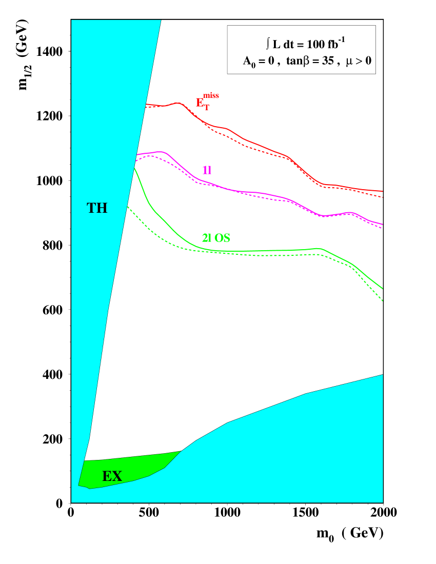
Figure 28: Effects of pile-up on the reach contours with 100 fb^-1 for Set 4. The solid line denotes contours obtained without pile-up, dashed line refers to pile-up added to signal samples.

7 Conclusions

The main conclusions of our study are the following $:$ within the SUGRA model investigated SUSY would be detectable through an excess of events over SM expectations up to masses m${}_{\tilde{q}}$ $\sim$ m${}_{\tilde{g}}$ $\sim$ 2.5 TeV with 100 fb^-1. This means that the entire plausible domain of EW-SUSY parameter space for most probable values of tan$\beta$ can be probed. Furthermore, the S/B ratios are $>$ 1 everywhere in the reachable domain of parameter space (with the appropriate cuts) thus allowing a study of kinematics of $\tilde{q}$, $\tilde{g}$ production and obtaining information on their masses. The cosmologically interesting region $\Omega h^{2}\leq$ 1, and even more so the preferred region 0.15 $\leq$ $\Omega h^{2}\leq$ 0.4, can be entirely probed.

8 Acknowledgements

We would like to thank prof. Daniel Huss for the support of this work and prof. Daniel Denegri for his advices and fruitful discussions. We also thank Alexandre Nikitenko for help in CMSIM drawings of mSUGRA events.

References

- [1] H. Baer, C.-H. Chen, F. Paige and X. Tata, Phys.Rev. D52, 2746 (1995); Phys.Rev. D53, 6241 (1996).
- [2] CMS collaboration, Technical Proposal, CERN/LHCC 94-38.
-
[3]
S. Abdullin, CMS TN/96-095,
S. Abdullin, Ž. Antunović and M. Dželalija, CMS Note 1997/016. - [4] H. Baer, C.-H. Chen, R. Munroe, F. Paige and X. Tata, Phys.Rev. D51, 1046 (1995).
- [5] H.Baer et al., FSU-HEP-980204, hep-ph/9802441.
- [6] H. Baer and M.Brhlik, Phys.Rev. D57, 567 (1998).
- [7] W. de Boer, IEKP-KA/97-03, hep-ph/9705309.
- [8] F. Paige and S. Protopopescu, in Supercollider Physics, p. 41, ed. D. Soper (World Scientific, 1986); H. Baer, F. Paige, S. Protopopescu and X. Tata, in Proceedings of the Workshop on Physics at Current Accelerators and Supercolliders, ed. J. Hewett, A. White and D. Zeppenfeld (Argonne National Laboratory, 1993).
-
[9]
S. Abdullin, A. Khanov and N. Stepanov, CMS TN/94-180
(see also /afs/cern.ch/user/a/abdullin/public/cmsjet/4.5/cmsjet4504_guide.ps). - [10] C. Charlot et al., CMS TN/93-63.
- [11] http://cmsdoc.cern.ch/cmsim/pictures/cmsim_events.html .
- [12] T. Sjöstrand, Computer Physics Commun. 39 (1986) 347; T. Sjöstrand and M. Bengtsson, Computer Physics Commun. 43 (1987) 367; H.U. Bengtsson and T. Sjöstrand, Computer Physics Commun. 46 (1987) 43; T. Sjöstrand, CERN-TH.7112/93.
- [13] H. Baer, M. Brhlik, D. Castao and X. Tata, Phys.Rev. D58, 015007 (1998).
- [14] M.S. Alam et al., (CLEO collaboration), Phys.Rev.Lett D74, 2885 (1995).
- [15] H. Baer, M. Brhlik, Phys.Rev. D55, 3201 (1997).