Accelerated convergence of perturbative QCD by optimal conformal mapping of the Borel plane

Irinel Caprini

National Institute of Physics and Nuclear Engineering, POB MG 6, Bucharest,

R-76900 Romania

and

Jan Fischer

Institute of Physics, Academy of Sciences of the Czech Republic, 182 21 Prague 8,

Czech Republic

The technique of conformal mappings is applied to enlarge the convergence domain of the Borel series and to accelerate the convergence of Borel-summed Green functions in perturbative QCD. We use the optimal mapping, which takes into account the location of all the singularities of the Borel transform as well as the present knowledge about its behaviour near the first branch points. The determination of $\alpha_{s}(m_{\tau}^{2})$ from the hadronic decay rate of the $\tau$-lepton is discussed as an illustration of the method.

1 Introduction

The behaviour of the large order terms in perturbative quantum field theory has been a subject of permanent interest [1]-[9]. Recently, this problem received much attention in the case of QCD [10]-[20]. As is known, the creation of instanton-antiinstanton pairs and certain classes of Feynman diagrams are responsible for a factorial increase of the large order coefficients of the perturbative expansion of the QCD Green functions, making this series divergent in the mathematical sense. Moreover, the growth of the large-order coefficients is so dramatic that, when combined with other difficult circumstances (like their non-alternating sign and the extraordinarily small analyticity domain of the Green functions in the coupling variable [9]), it leads to the situation that some of the usually efficient summation techniques [21] are not applicable. One of them, the Borel summation, was very much investigated in the recent time. The growth of the large order perturbative coefficients of the QCD Green functions leads, under certain conditions, to Borel transforms with singularities in the Borel plane that make the integral defining the Green function by the Laplace transform ill-defined. Of course, as discussed in [19], the Borel technique is not the only mathematical method by which a divergent series can be summed, but an ambiguity emerges in every summation method, once it is discovered in one of them. The real source of nonuniqueness consists in a missing piece of information about the quantities to be calculated, which adopts different forms in different summation methods, but has to be added to eliminate the ambiguity.

In QCD the Borel nonsummability originates from the infrared regions of the Feynman diagrams, where nonperturbative effects play also an important role. Therefore it is natural to assume that the ambiguities of perturbation theory must be compensated by nonperturbative contributions. In fact, it turns out that general concepts like analyticity, renormalization group or specific properties of the QCD vacuum are unavoidable when discussing the large order behaviour of perturbation theory [4],[9],[19]. As an example, we recall that the argument given by ’t Hooft [9] for the Borel nonsummability of QCD relies on nonperturbative properties, mainly the momentum plane analyticity combined with renormalization group invariance. So the perturbative and the nonperturbative regimes of the theory cannot be separated, and their interplay is very clear when attempting to perform the summation of the large orders of perturbation theory. The Borel plane is particularly suitable for discussing this aspect, since the singularities of the Borel transform offer a very intuitive measure of the ambiguities of the perturbation theory and suggest the way to compensate them. The properties of these singularities in some approximations (like massless QCD in the large $\beta_{0}$ limit, when they are poles [13]) were used recently to provide estimates of the truncation error in the theoretical determinations of some accurately measured quantities.

A natural question is whether it is possible to improve the accuracy of the Borel summation using the first Taylor coefficients of the Borel transform known from the explicit low order calculations, supplemented with some (approximate) information about its singularities in the Borel plane. We address this question in the present paper. We use as input the assumption that, for suitable QCD amplitudes, there are no other singularities in the Borel plane than those located on the real axis, at a nonvanishing distance from the origin. The precise nature and strength of these singularities is not known in general, except for the nearest ones, which can be characterized (at least approximately) by using general principles. As discussed in [4], the singularities of the Borel transform require the introduction of higher dimensional operators, which ensure the compensation of the ambiguities present in the usual perturbative terms by the ambiguities inherent in their Wilson coefficients. This allows one also to infer a universal behaviour of the Borel transform near the first ultraviolet renormalon [20]. On the other hand, as discussed in [10], the location and nature of the first infrared renormalon can be plausibly predicted too, by nonperturbative arguments. In our approach, we take as input this knowledge about the first ultraviolet and infrared renormalons.

Our purpose was to exploit in an optimal way this information, in order to improve the accuracy of the Borel summation in the frame of a specific prescription of handling the singularities of the Borel transform. To this end we use the analytic continuation of the Borel transform outside the circle of convergence of the Taylor expansion, achieved by the technique of conformal mapping. As is known, the conformal mappings are very suitable for accelerating the convergence of power series. The existence of an optimal expansion, with the largest convergence domain and the best asymptotic convergence rate, was proven in [22] a long time ago. The method is applicable if the position of the singularities of the function to be approximated is known or can be reasonably guessed, which is the case in many situations in particle physics.

In the context of the Borel summation in quantum field theory, the conformal mappings were first considered in [5]-[8]. More recently, the method was applied in [23]-[24] to the Borel transform of QCD Green functions, following a suggestion made in [10]. The purpose was to estimate (and possibly reduce) the influence of the first ultraviolet renormalon and of the associated power corrections on observable quantities, by using a variable in which this singularity is pushed further away from the integration range of the Borel transform. However, from the point of view of the convergence rate the mapping used in [23]-[24] is not optimal, since it takes into account only a part of the singularities of the Borel transform, the ultraviolet (UV) renormalons. By using an optimal treatment, which takes into account also the infrared (IR) renormalons and the behaviour near the first singularities, an increased convergence rate and consequently a smaller truncation error are to be expected.

The objective of our work is to establish whether the optimal mapping technique is numerically relevant in the Borel plane for situations of physical interest (we mention alternative attempts to enlarge the convergence domain of the Borel transform, based on Padé approximants [25]). To illustrate our discussion we consider, as in [23], the Adler function of the massless QCD vacuum polarization and the determination of the strong coupling constant $\alpha_{s}(m_{\tau}^{2})$ from the hadronic $\tau$ decay rate. In the next section we briefly review some properties of the Adler function and of its Borel transform. In section 3 we present the technique of optimal conformal mapping and investigate its efficiency in the Borel plane on several mathematical models which simulate the physical situation. We discuss also the determination of the strong coupling constant $\alpha_{s}(m_{\tau}^{2})$ using the present technique. Some conclusions are formulated in section 4.

2 The Adler function and its Borel transform

We consider the correlator

$$i\int{\rm d}^{4}x\,e^{iq\cdot x}\,\langle 0|\,T\,\{V^{\mu}(x),V^{\nu}(0)^{\dagger}\}\,|0\rangle=(q^{\mu}q^{\nu}-g^{\mu\nu}q^{2})\,\Pi(s)\,,$$ (1)

where $s=q^{2}$ and $V^{\mu}=\bar{q}\gamma^{\mu}q$ is the current of a massless quark. From the general principles of causality and unitarity it follows that the amplitude $\Pi(s)$ is an analytic function of real type in the complex plane $s$, cut along the real positive axis from the threshold $4m_{\pi}^{2}$ of hadron production to infinity. It is convenient to define the Adler function

$$D(s)=-{{\rm d}\over{\rm d}s}\,\Pi(s)\,,$$ (2)

which is ultraviolet finite and is also analytic in the complex $s$-plane cut above the unitarity threshold. This function was much investigated lately in connection with the determination of the strong coupling constant $\alpha_{s}(m_{\tau}^{2})$ from the hadronic decay of the $\tau$ lepton [14],[17], [26] - [29]. The hadronic decay width, normalized to the leptonic one, is defined as

$$R_{\tau}={\Gamma(\tau\to\nu_{\tau}+\mbox{hadrons})\over\Gamma(\tau\to\nu_{\tau}\,e\,\bar{\nu}_{e})}=\int\limits_{0}^{m_{\tau}^{2}}\!{\rm d}s\,{{\rm d}R_{\tau}(s)\over{\rm d}s}\,,$$ (3)

where the inclusive hadronic spectrum ${\rm d}R_{\tau}(s)/{\rm d}s$ is related to the spectral part of the correlator (1):

$${{\rm d}R_{\tau}(s)\over{\rm d}s}={3(1+\delta_{\rm EW})\over\pi m_{\tau}^{2}}\,\bigg{(}1-{s\over m_{\tau}^{2}}\bigg{)}^{2}\bigg{(}1+{2s\over m_{\tau}^{2}}\bigg{)}\,\mbox{Im}\,\Pi(s+i\epsilon)\,.$$ (4)

The factor $\delta_{\rm EW}\simeq 0.0194$ accounts for electroweak radiative corrections. The decay rate (3) was measured recently with great accuracy [31], [32].

Using the analyticity properties of the function $\Pi(s)$ in the momentum plane, the relation (3) can be transformed by a Cauchy relation into

$$R_{\tau}={3(1+\delta_{\rm EW})\over 2\pi i}\,\oint{{\rm d}s\over s}\bigg{(}1-{s\over m_{\tau}^{2}}\bigg{)}^{3}\bigg{(}1+{s\over m_{\tau}^{2}}\bigg{)}\,\,D(s)\,,$$ (5)

where the integration runs along a closed contour in the complex plane, taken usually to be the circle $|s|=m^{2}_{\tau}$.

The relation (5) is the starting point for the computation of the $\tau$ hadronic width in perturbative QCD. At complex values of $s$ the Adler function admits the formal renormalization-group-improved expansion

$$D(s)=1+\sum_{n=1}^{\infty}\,D_{n}\,\bigg{(}{\alpha_{s}(-s)\over\pi}\bigg{)}^{n}\,.$$ (6)

The strong coupling $\alpha_{s}(\mu^{2})$ satisfies the renormalization-group equation

$$\mu^{2}{{\rm d}\alpha_{s}(\mu^{2})\over{\rm d}\mu^{2}}=-\alpha_{s}(\mu^{2})\sum_{n=0}^{\infty}\beta_{n}(\alpha_{s}(\mu^{2}))^{n+1}\,,$$ (7)

with the first coefficients $\beta_{n}$ defined in terms of the number $n_{f}$ of quark flavours as

$$\beta_{0} = {33-2n_{f}\over 12\pi}$$

$$\beta_{1} = {153-19n_{f}\over 24\pi^{2}}\,.$$ (8)

The coefficients $D_{n}$ in the expansion (6) were computed for $n\leq 3$ [33]-[37]. In the $\overline{\rm MS}$ scheme with $n_{f}=3$ they are

$$D_{1} = 1\,,$$

$$D_{2} = 1.63982\,,$$

$$D_{3}^{\overline{\rm MS}} = 6.37101\,.$$ (9)

On the other hand, the large-order coefficients, $D_{n}$ for large $n$, have the generic factorial behaviour

$$D_{n}\approx C_{k}\,n!\,n^{\delta_{k}}\,\left({\pi\beta_{0}\over k}\right)^{n}+....$$ (10)

where the index $k$ takes the values: $-1,\pm 2,\pm 3....$.

In the Borel method of summation one defines the Borel transform of the Adler function as

$$B(u)=\sum_{n=0}^{\infty}\,b_{n}\,u^{n}\,,$$ (11)

where

$$b_{n}={1\over n!}\,{D_{n+1}\over(\pi\beta_{0})^{n}}\,=\,{\widetilde{D}_{n+1}\over n!}\,.$$ (12)

Then $D(s)$ can be expressed formally in terms of $B(u)$ by the Laplace transform

$$D(s)=1+{1\over\pi\beta_{0}}\,\int\limits_{0}^{\infty}\!{\rm d}u\,B(u)\,\exp\bigg{(}-{u\over\beta_{0}\alpha_{s}(-s)}\bigg{)}\,.$$ (13)

To illustrate our technique we shall use also a Borel-summed expression for the hadronic decay rate $R_{\tau}$. Such an expression was obtained in [23] by inserting in (5) the Borel representation (13) of the Adler function and performing the integration along the circle $|s|=m_{\tau}^{2}$ in the one-loop approximation

$$\alpha_{s}(-s)\,={1\over\beta_{0}\ln(-s/\Lambda^{2})}\,$$ (14)

of the running coupling. This procedure gives [23]

$$R_{\tau}\,=\,3(1+\delta_{{\rm EW}})\left[1+{1\over\pi\beta_{0}}\int_{0}^{\infty}{\rm d}u\exp\bigg{(}-{u\over\beta_{0}\alpha_{s}(m_{\tau}^{2})}\bigg{)}\,B(u)\,F(u)\,\right]\,,$$ (15)

where

$$F(u)={-12\,\sin(\pi u)\over\pi\,u(u-1)(u-3)(u-4)}\,.$$ (16)

We shall use (15) as a starting point for a determination of $\alpha_{s}(m_{\tau}^{2})$ in Section 3.

The growth (10) of the Taylor coefficients $D_{n}$ leads to the dominant behaviour

$$B(u)\approx C_{k}\,\Gamma\,(\delta_{k}+1)\,(1-{u\over k})^{-\delta_{k}-1}+...,$$ (17)

which shows that the function $B(u)$ becomes singular at the points $u=k$, with $k=-1,\pm 2,\pm 3...$. The precise values of $C_{k}$ and $\delta_{k}$ are not known in general. However, from general arguments it was shown that the nature of the first branch points of the Borel transform is universal [10], [20]. More precisely, near the first UV renormalon at $u=-1$ the Borel transform behaves as

$$B(u)\,\simeq\,r_{1}\,(1+u)^{-\gamma_{1}}\,,$$ (18)

where [20]

$$\gamma_{1}=3-{\beta_{1}\over\beta_{0}^{2}}+\lambda_{1}\,.$$ (19)

Here $\lambda_{1}$ is a parameter depending on the number of flavours, which reflects the mixing of higher dimensional operators in the renormalization group equations [20]. Similarly, near the first IR renormalon at $u=2$ the behaviour is

$$B(u)\,\simeq\,r_{2}\,(2-u)^{-\gamma_{2}}\,\,,$$ (20)

where [10]

$$\gamma_{2}=1+2{\beta_{1}\over\beta_{0}^{2}}\,.$$ (21)

Using the first coefficients $\beta_{i}$ from (2) and the parameter $\lambda_{1}$ given in [20] (equal to 0.379 for $n_{f}=3$ and 0.630 for $n_{f}=5$) we obtain

$$\gamma_{1}=2.589\,,\,\,\gamma_{2}=2.580$$ (22)

for $n_{f}=3$, and

$$\gamma_{1}=2.972\,,\,\,\gamma_{2}=2.316$$ (23)

for $n_{f}=5$. We emphasize that only the nature of the first renormalons is known, and nothing can be said about the residues $r_{1}$ and $r_{2}$ appearing in (18) and 20, respectively.

Strictly speaking, the integrals (13) or (15) have nothing to do with the summation of the perturbative series, because one condition of the Borel theorem (the existence of the analytic continuation in the $\alpha_{s}$ plane from the convergence disk to an infinite strip around the positive real semiaxis) is not satisfied [21], [9]. This can be seen from the singularities of the Borel transform given in (17): the poles situated on the real positive axis (IR renormalons) make the integrals (13) and (15) ambiguous. In order to compute them a prescription has to be adopted, by suitably choosing the integration contour in order to avoid the singularities. But this is not the Borel summation. Different prescriptions give different results, and a measure of the intrinsic ambiguity of the perturbation expansion is given by the difference between these results, if no a priori arguments in favor of a certain choice exist.

A prescription adopted by several authors [8], [14], [17] is the “principal value” (PV), defined as

$${\rm PV}\int_{0}^{\infty}{\rm d}u\exp\left(-{u\over a_{s}}\right)f(u)\equiv{1\over 2}\,\left[\int_{{\cal C_{+}}}{\rm d}u\exp\left(-{u\over a_{s}}\right)f(u)\,{\rm d}u\,+\int_{{\cal C}_{-}}{\rm d}u\exp\left(-{u\over a_{s}}\right)f(u)\right]\,,$$ (24)

where ${\cal C}_{\pm}$ are two lines parallel to the real axis, slightly above and below it. This definition is a generalization to arbitrary singularities of the Cauchy principal value of simple poles, and has the advantage of yielding a real result when $a_{s}$ is real. Although this prescription is not unique, we adopted it as a working hypothesis.

We applied the definition (24) for computing the Borel-summed Adler function (given by the Laplace integral (13)), and the hadronic $\tau$ decay rate (given by (15)). In the first case the parameter $a_{s}$ is related to the running coupling $\alpha_{s}(-s)$ (and may be complex if $s$ is complex or in the Minkowskian region $s>0$), while in the second case it is proportional to $\alpha_{s}(m_{\tau}^{2})$. We use as input the first Taylor coefficients of $B(u)$ (known from (12) and the calculated values (2)), supplemented by the knowledge on the location and the nature of singularities of this function. As discussed in the Introduction, our purpose is to improve the accuracy of the calculation by the technique of conformal mappings, which exploits in an optimal way this input information.

3 Optimal conformal mapping of the Borel plane

3.1 Remarks on the theory

The use of conformal mappings for improving the convergence of power series in particle physics was discussed for the first time in Ref. [22]. The problem formulated in [22] was to find the optimal conformal transformation which minimizes the asymptotic truncation error of a power series, taking into account the location of the singularities of the function to be approximated. First we briefly describe the results obtained in [22]. We consider a function $f(u)$ analytic in a domain $\cal D$ of the complex $u$ plane containing the origin, and write its Taylor series truncated at a finite order $N$ as

$$f^{(N)}(u)=\sum_{n=0}^{N}f_{n}\,u^{n}\,.$$ (25)

According to general theory, the series (25) converges, for $N\to\infty$, inside the circle passing through the nearest singularity of the function $f(u)$ in the complex plane, the rate of convergence at a point $u$ situated inside the circle being that of the geometrical series in powers of ${r\over R}$, where $r=|u|$ and $R$ is the radius of the convergence circle. Therefore, the convergence rate is strongly influenced by the distance of the singularities of $f(u)$ from the origin, and can be improved by using a suitable change of variable, in which the singularities are pushed further away from the region of interest.

Let us consider a conformal mapping $w=w(u)$ of the plane $u$ onto the plane $w$, such that $w(0)=0$, and write the truncated Taylor expansion of the function $f(u)$ in the variable $w$:

$$f^{(N)}_{w}(u)=\sum_{n=0}^{N}c_{n}\,w^{n}\,.$$ (26)

As pointed out in [22], the best asymptotic rate of convergence of this series in a certain region of the complex plane is achieved when $w$ is such a transformation of the $u$ plane that the corresponding ratio ${r\over R}$ is minimal for every point in that region. According to the theorem proven in [22] this is realized by a conformal mapping $w(u)$ which maps the whole analyticity domain $\cal D$ of the function $f(u)$ in the $u$ plane into the interior of a circle in the plane $w$. The proof of the theorem is based on the fact that the circle is the domain of convergence for power series, and on the Schwartz lemma, which implies that the larger the domain mapped inside the circle, the better is the asymptotic rate of convergence (for details see [22]).

In what follows we shall apply this technique to the Borel transform $B(u)$ of the Adler function. The nearest singularities of the function $B(u)$ are situated at $u=-1$ and $u=2$ and the power expansion (11) converges only inside the circle $|u|<1$ passing through the first UV renormalon. It is easy to see that the optimal conformal mapping in the sense explained above is given in our case by

$$w={\sqrt{1+u}-\sqrt{1-u/2}\over\sqrt{1+u}+\sqrt{1-u/2}}\,.$$ (27)

By this mapping, the complex $u$ plane cut along the real axis for $u>2$ and $u<-1$ is mapped onto the interior of the circle $|w|\,<\,1$ in the complex $w$-plane, the origin $u=0$ of the $u$ plane becoming the origin $w=0$ of the $w$ plane, and the upper (lower) lips of the cuts are mapped onto the upper (lower) semicircle in the plane $w$. Particularly, all the singularities of the Borel transform, the UV and IR renormalons, are now situated on the boundary of the unit disc in the $w$ plane, all at equal distance from the origin. The Taylor expansion of the Borel transform in powers of $w$,

$$\tilde{B}_{w}^{(N)}(u)=\sum_{n=0}^{N}\tilde{c}_{n}\,w^{n}\,,$$ (28)

will converge for $N\to\infty$ up to points close to the renormalons. This is a considerable improvement with respect to the usual expansion (11), whose convergence in the Borel plane is limited by the circle reaching the first UV renormalon. The requirement of convergence of (28) on this disc implies the holomorphy of the expanded function on the disc. In this way, the expansion in powers of $w(u)$ makes full use of the analyticity property that is universally (but tacitly) assumed in all QCD considerations, namely that there are no singularities in the Borel plane other than those situated on the real axis, at a nonvanishing distance from the origin. This essential, additional assumption has, to our knowledge, not been explicitly used.

For comparison we give the conformal mapping used in [23]- [24],

$$z={\sqrt{1+u}-1\over\sqrt{1+u}+1}\,,$$ (29)

which maps the $u$ plane cut along $u<-1$ onto the interior of the unit circle in the $z$ plane. In the $z$ plane the UV renormalons are situated along the boundary of the unit circle $|z|=1$, but the IR renormalons are situated inside this circle. As noticed in [24], pushing away the ultraviolet renormalons by (29) has a price in moving the first infrared renormalon (and actually, the whole positive real semiaxis) closer to the origin. This is why the convergence domain of the power series in $z$ is limited by the first IR renormalon and, as a consequence, the convergence rate of the series in powers $z$ will be worse than that obtained with the optimal variable (27). The use of the optimal conformal mapping (27) is therefore highly desirable, because it does not suffer from this shortcoming, placing all the renormalons onto the circumference of the unit disk.

As was noticed in [38], a further improvement of the convergence rate can be reached if some information about the nature of the singularities of the expanded function $f(u)$ is available. The idea is that the power variable $w(u)$, taken as a function of $u$, should resemble $f(u)$ as much as our knowledge of $f(u)$ allows it. (As it was put in [22], if we were to know $f$ exactly, the most rapidly convergent expansion would be that in powers of $f$ itself, in which case it would reduce to the identity $f\equiv f$.)

In practice, however, our knowledge of the expanded function is only approximative. For instance, as discussed above, we know that near the branch points $u=-1$ and $u=2$ the function $B(u)$ behaves like $(u+1)^{-\gamma_{1}}$ and $(2-u)^{-\gamma_{2}}$ respectively, with the $\gamma_{i}$ real positive numbers. In this case it is convenient to expand the product $(u+1)^{\gamma_{1}}\,(2-u)^{\gamma_{2}}\,B(u)$ in powers of the optimal variable $w$ defined in (27), and introduce then explicitly the singular factors. The expansion of the function $B(u)$ will have the form

$$\hat{B}_{w}^{(N)}(u)={1\over(u+1)^{\gamma_{1}}(2-u)^{\gamma_{2}}}\sum_{n=0}^{N}\hat{c}_{n}\,w^{n}\,.$$ (30)

The singularities themselves may survive as positive powers $(u+1)^{\gamma_{1}}$ and $(2-u)^{\gamma_{2}}$, the bonus nevertheless being that the positive exponents $\gamma_{i}$ keep the values of the function

$$(u+1)^{\gamma_{1}}(2-u)^{\gamma_{2}}B(u)$$ (31)

finite near $u=u_{1}$ and $u=u_{2}$, which softens their numerical impact. This step will imply no large-order improvement of the convergence rate (because the rate is given by the position of the nearest singularities), unless some of the two singularities is fully removed by it. But it may represent a considerable improvement at low orders, even if the nature of the nearest singularities is known only approximately. A nice example of efficiency of this approach in practice was presented by Soper and Surguladze in [24].

3.2 Discussion of mathematical models

We tested the practical efficiency of the conformal mapping (27) for a number of functions having logarithmic or power branch points at $u=-1$ and $u=2$. We took functions close to the physical situation as described in Section 2, i.e. we started from a ”perturbative” expansion of the form

$$B^{(N)}(u)=\sum_{n=0}^{N}\,b_{n}\,u^{n}\,,$$ (32)

with low values of $N$. The expansion (28) in terms of the variable $w$ is obtained by replacing $u$ in (32) with the expansion

$$u^{(N)}_{w}=\sum_{n=1}^{N}C_{n}w^{n}$$ (33)

which follows from the inverse of (27), and keeping only terms up to the order $N$ (i.e. $(u^{(N)}_{w})^{N}=C_{1}^{N}w^{N}$, etc). The numerical values of the first coefficients $C_{n}$ are:

$$C_{1}={8\over 3}\,,\,C_{2}={16\over 9}\,,\,C_{3}=-{40\over 27}\,,\,C_{4}=-{224\over 81}\,,\,C_{5}=-{88\over 243}\,...$$ (34)

For comparison, the expansion in powers of the variable $z$ given in (29) is obtained using

$$u^{(N)}_{z}=\sum_{n=1}^{N}\bar{C}_{n}z^{n}\,$$ (35)

with the numerical values [23]

$$\bar{C}_{1}=4\,,\,\bar{C}_{2}=8\,,\,\bar{C}_{3}=12\,,\,\bar{C}_{4}=16\,,\,\bar{C}_{5}=20\,...$$ (36)

We first computed the model functions and their various approximants at points $u$ inside the analyticity region, near the origin of the Borel plane. In most of the cases investigated the expansions in powers of the optimal variable $w$ approximated the exact functions much better than the standard expansion (32) or the series in powers of the $z$ variable. This feature was visible even with a few terms in the expansion. Actually, as we discussed in the previous Section, for the physical applications we are interested in the calculation of Laplace integrals like (13) or (15). We evaluated this integral, with the generalized principal value prescription defined in (24) for a large number of functions of physical interest. We consider as an example the function

$$B(u)={r_{1}\over(1+u)^{\gamma_{1}}}+{r_{2}\over(2-u)^{\gamma_{2}}}+\sum_{n=3}^{N_{IR}}{r_{n}\over(n-u)^{\gamma_{n}}}\,,$$ (37)

which simulates the contribution of a few renormalons. The principal value (24) of the Laplace integral was computed numerically with great accuracy. In order to check the computations we used the relation [39]

$$\lim_{\epsilon\to 0}\int_{0}^{\infty}{\rm d}u{\exp(-u/a_{s})\over(u+b+i\epsilon)^{\nu}}\,=\,a_{s}^{1-\nu}{\rm e}^{b/a_{s}}\Gamma(-\nu+1,b/a_{s})\,,\,{\rm Re}\,a_{s}>0\,,$$ (38)

where $\epsilon>0$ and $\Gamma(\nu,z)$ is the incomplete gamma function [39], analytically continued from the region ${\rm Re}\,z\,>0$ to the whole complex plane $z$ cut along the negative real axis. For integer $\nu$ this can be expressed equivalently as [40]

$$\lim_{\epsilon\to 0}\int_{0}^{\infty}{\rm d}u{\exp(-u/a_{s})\over(u+b+i\epsilon)^{n}}\,=\,{{\rm e}^{b/a_{s}}\over b^{n-1}}E_{n}(b/a_{s})\,,\,{\rm Re}\,a_{s}>0\,,$$ (39)

in terms of the exponential integral functions $E_{n}(z)$. Actually, as seen from (37), in the physical case the denominators must be defined so as to give the correct cut structure of the Borel transform. This case is obtained from (39) as

$$\lim_{\epsilon\to 0}\int_{0}^{\infty}{\rm d}u\,{\exp(-u/a_{s})\over(|b|-u-i\epsilon)^{n}}\,=\,{{\rm e}^{b/a_{s}}\over-|b|^{n-1}}E_{n}(b/a_{s})\,,$$ (40)

where $b=-|b|$.

As a side remark, we mention that the above relations are useful for defining the principal value prescription for arbitrary values of $a_{s}$. First, by means of repeated integration by parts in (39) we can express the left hand side as [39]

$$\int_{0}^{\infty}{\rm d}u{\exp(-u/a_{s})\over(u+b+i\epsilon)^{n}}\,=\sum_{m=1}^{n-1}{(m-1)!\over(n-1)!}\,{(-a_{s})^{1-n+m}\over b^{m}}\,+\,{(-a_{s})^{1-n}\over(n-1)!}\int_{0}^{\infty}{\rm d}u{\exp(-u/a_{s})\over(u+b+i\epsilon)}\,,$$

$${\rm Re}\,a_{s}>0\,.$$ (41)

We now apply the definition (24) of the principal value and use the symbolic relation

$${1\over(u+b\pm i\epsilon)}={\rm PV}{1\over(u+b)}\,\mp\,i\pi\delta(u+b)\,.$$ (42)

in the last term in (3.2). We obtain thus the following expression of the principal value

$${\rm PV}\int_{0}^{\infty}{\rm d}u{\exp(-u/a_{s})\over(u+b)^{n}}\,=\,{{\rm e}^{b/a_{s}}\over b^{n-1}}E_{n}(b/a_{s})\,+\,i\pi{(-a_{s})^{1-n}\over(n-1)!}{\rm e}^{b/a_{s}}\,,\,\,{\rm Re}\,a_{s}>0\,.$$ (43)

For real values of $a_{s}$ the last term in the above relation is purely imaginary and compensates the imaginary part of the first term. In this case the definition (43) amounts therefore to taking the real part of the right hand side of (39). For complex $a_{s}$, when the last term in (43) has also a nonvanishing real part, the compensation does not occur, and the result is complex. As discussed below Eq.(24), complex values of $a_{s}$ appear in the Borel summation of the Green functions in the complex momentum plane or in the timelike region. For some Minkowskian quantities a definition of the principal value, based on physical arguments, was proposed in [14]. The above expression (43) is general and covers all these cases.

 

Figure 1: Laplace integral for the model (37) as a function of $a_{s}$: exact values (a); perturbation expansion (b); expansion in powers of $z$ (c); improved expansion in powers of $z$ (d); expansion in powers of $w$ (e); improved expansion in powers of $w$ (f). The series are truncated at $N=3$.

In Fig.1 we give for illustration the results of our analysis for the model function (37) with the parameters: $r_{1}=1,r_{2}=4,r_{n}=0\,,n\geq 3,\gamma_{1}=2.5,\gamma_{2}=2.5$, and $a_{s}$ in the range (0.1-0.9). The Laplace integral of the exact function (37) is indicated together with the results given by its ordinary perturbative expansion (truncated at $N=3$), and the expansions accelerated by the conformal mappings $z$ and $w$, both in the simple versions and with the improvement explained in (30). To simulate the physical situation in a more realistic way, we assumed that the nature of the first singularities is not exactly known and used in the improved version (30) the product of $B(u)$ with the factors $(u+1)^{2.0}(2-u)^{2.0}$, which do not compensate exactly the singularities of the model function (37).

As seen from Fig.1, the combined technique of conformal mapping and the explicit treatment of the branch points, supposing that some (approximate) information about the behaviour of the function near the first singularities is available, improves the accuracy of the Borel integral, especially for large $a_{s}$. The values $a_{s}\approx 0.2-0.3$ (of interest in the hadronic $\tau$ decay) are on the boundary of the region for which the improvement is significant at this order, $N=3$. We notice that a major part of the improvement is brought by the separate treatment of the branch points, according to (30), especially at low $N$. Even the standard expansion in powers of the Borel variable $u$ gives good results if the nature of the lowest singularities, assumed to be exactly known, is treated explicitly as above. However, when the behaviour near the first singularities is known only approximately, the expansion in the optimal variable gives in general the best approximation, especially when the order $N$ of the truncation is increased.

$N$	$(a)$	$(b)$	$(c)$	$(d)$	$(e)$	$(f)$
3	0.35	0.530	0.50	0.546	0.47	0.5596
4	0.90	0.610	0.540	0.5625	0.64	0.5701
5	–0.10	0.5732	0.547	0.5722	0.5457	0.5701
6	2.2	0.516	0.5631	0.5783	0.613	0.56518
7	$-$3.6	0.82	0.5743	0.582	0.63	0.56518
8	13	$-$0.12	0.587	0.584	0.515	0.563102
9	$-$40	2.3	0.599	0.584	0.64	0.563100
10	143	$-$3.4	0.613	0.583	0.503	0.563470
11	$-$541	9.5	0.63	0.581	0.540	0.563467
12	2 $10^{3}$	$-$19	0.64	0.5776	0.590	0.563783
15	$-$2 $10^{5}$	199	0.72	0.56400	0.5783	0.563713
20	2 $10^{9}$	$-$8 $10^{3}$	1.1	0.530	0.582	0.563689
25	$-$4 $10^{13}$	3 $10^{5}$	2.7	0.48	0.5687	0.563681
30	2 $10^{18}$	$-$5 $10^{7}$	13	0.43	0.559754	0.563682

Table 1: Approximations of the Laplace integral for $a_{s}=0.3$ for different truncation orders: $(a)$ expansion in powers of $u$; $(b)$ “improved” expansion in powers of $u$; $(c)$ expansion in powers of $z$; $(d)$ “improved” expansion in powers of $z$; $(e)$ expansion in powers of $w$; $(f)$ “improved” expansion in powers of $w$. The exact value is $D(0.3)=0.563683$. The results close to the exact value are indicated with a greater number of digits.

We illustrate this fact in Table 1, where we indicate the Laplace integral for $a_{s}=0.3$, of the function (37) with $\gamma_{1}=\gamma_{2}=2.5$ as a function of the truncation order $N$, for different types of expansions. The “improved” expansions were obtained now by expanding in powers the product of $B(u)$ with the factors $(u+1)^{1.5}(2-u)^{1.5}$, close but not identical with the actual behaviour of (37).

For larger values of $a_{s}$ the improved accuracy obtained by using the optimal mapping is even more impressive. Some results are presented in Table 2 and in Table 3, for $a_{s}=0.5$ and $a_{s}=0.8$, respectively. Similar results were obtained also for model functions with more singularities on the real axis.

$N$	$(a)$	$(b)$	$(c)$	$(d)$	$(e)$	$(f)$
3	$-$0.51	1.04	0.925	1.01	0.739	0.97
5	$-$15	1.9	1.22	1.05	1.7	0.8769
10	4 $10^{4}$	$-$75	2.4	0.8412	2.2	0.857092
12	2 $10^{6}$	349	3.6	0.678	1.8	0.853068
15	$-$9 $10^{8}$	3 $10^{3}$	8.2	0.37	1.6	0.852614
20	8 $10^{13}$	$-$1 $10^{5}$	56	$-$0.27	2 $10^{-3}$	0.853263
25	$-$2 $10^{19}$	1 $10^{8}$	597	$-$1.06	0.59	0.853463
30	1 $10^{25}$	$-$3 $10^{13}$	8 $10^{3}$	$-$2.0	1.5	0.853438

Table 2: The same as in Table 1, for $a_{s}=0.5$. The exact value is $D(0.5)=0.853427$.

A closer look at the Tables 1, 2, and 3 reveals that there are essentially three circumstances affecting the convergence properties: (i) the use of a convenient (including the optimal) conformal mapping, (ii) explicit (but, in practice, approximative) account of the branch point singularities, and (iii) exponential damping of the integrand by $\exp\left(-{u/a_{s}}\right)$.

$N$	$(a)$	$(b)$	$(c)$	$(d)$	$(e)$	$(f)$
3	$-$9.1	1.9	1.7	1.34	1.8	1.00
5	$-$296	6.7	3.2	1.13	6.1	0.61
10	8 $10^{6}$	$-$381	17	$-$0.442	13	0.69528
12	9 $10^{8}$	$-$2 $10^{3}$	41	$-$1.35	$-$18	0.6873
15	$-$2 $10^{12}$	2 $10^{4}$	178	$-$3.0	$-$22	0.70106
20	1 $10^{19}$	5 $10^{6}$	3 $10^{3}$	$-$6.2	$-$7.1	0.69741
25	$-$2 $10^{24}$	3 $10^{12}$	6 $10^{4}$	$-$10	21	0.69580
30	4 $10^{30}$	$-$3 $10^{18}$	2 $10^{6}$	$-$14	$-$12	0.696204

Table 3: The same as in Table 1, for $a_{s}=0.8$. The exact value is $D(0.8)=0.696408$.

The effect of the factor (i) can be seen from the fact that, in each of the Tables, the column (c) possesses better convergence properties than the column (a), and the column (e) has better properties than the column (c). The effect of (ii) is seen from the fact that, again in all three Tables, the columns (f), (d) and (b) have better convergence properties than the columns (e), (c) and (a), respectively. As concerns the point (iii), we see from Table 3 that the salutary effect of the optimal conformal mapping is most spectacular when the damping of the exponential function $\exp\left(-{u/a_{s}}\right)$ is the weakest, i.e., when $a_{s}$ has the highest value, $a_{s}=0.8$ in our case. Indeed, in this case, only the combined technique of the optimal conformal mapping and the explicit treatment of the branch points leads to numerical convergence, with steadily increasing accuracy up to $N=30$ by the least.

In the case of a stronger damping (Table 1), the role of the optimal conformal mapping combined with a careful regard to the branch point singularities is again important, but good results are obtained also by the other methods, the success varying with the perturbation order $N$ used; see the different columns (b) – (f) of Table 1 at different values of $N$. The asymptotic superiority of the optimal mapping (columns (e) and (f)) emerges at very high values of $N$; this mapping supersedes the other methods and turns out to be the best at least from $N=20$ on up to the highest value of $N$ shown in the Tables, $N=30$.

It is not excluded, on the other hand, that even the best series, column (f), will exhibit numerical indications of divergence at still higher orders; note that the singularities survive in some form because we (on purpose, in order to simulate real situations) had not completely removed them (see(ii)). Consequently, as the Borel integral path runs along the cut, which in the $w$ plane is mapped onto the boundary circle of the convergence disk, no convergence is warranted even in the column (f). It was already pointed out that for lower values of $a_{s}$, where the influence of infrared renormalons is more suppressed (see e.g. Table 1), results close to $D(0.3)$ are obtained even when other methods are used, see Table 1, sometimes only at lower values of $N$.

To further illustrate the use of the optimal conformal mapping introduced above, we investigated it in a model proposed in [23], adjusted to better simulate the physical situation. We assume the case when the Borel function is exactly given by

$$B_{true}(u)=1+\widetilde{D}_{2}u+{\widetilde{D}_{3}\over 2}u^{2}+[\widehat{B}(u)-\sum_{n=0}^{2}\hat{b}_{n}u^{n}]\,.$$ (44)

In this expression the parameters $\widetilde{D}_{2}$ and $\widetilde{D}_{3}$ are for the moment arbitrary and the numbers $\hat{b}_{n}$ are the Taylor coefficients of the expansion of $\widehat{B}$ around the origin:

$$\widehat{B}(u)=\sum_{n=0}^{\infty}\hat{b}_{n}u^{n}\,.$$ (45)

For $\widehat{B}(u)$ we choose the expression

$$\widehat{B}(u)={B_{0}(2)\over(1-u/2)}\,+\sum_{l=1}^{N_{UV}}{A_{0}(l)+A_{1}(l)u\over(1+u/l)^{2}}\,+\,\sum_{l=3}^{N_{IR}}{B_{0}(l)+B_{1}(l)u\over(1-u/l)^{2}}\,,$$ (46)

with

$$A_{0}(l) = {8\over 3}{(-1)^{l+1}(3l^{2}+6l+2)\over l^{2}(l+1)^{(}l+2)^{2}}$$

$$A_{1}(l) = {16\over 3}{(-1)^{l+1}(l+3/2)\over l^{2}(l+1)^{(}l+2)^{2}}$$

$$B_{0}(2) = 0$$

$$B_{0}(l) = -A_{0}(-l)\,\,;~{}~{}~{}~{}l\geq 3$$

$$B_{1}(l) = -A_{1}(-l)\,\,;~{}~{}~{}~{}l\geq 3\,.$$ (47)

The function $\widehat{B}(u)$ coincides actually with the Borel transform in the large $\beta_{0}$ limit [14], with finite numbers $N_{UV}$ and $N_{IR}$ of UV renormalons and IR renormalons, respectively. The meaning of the the model adopted above for $B_{true}$ is clear: it represents a function with the first 3 Taylor terms specified explicitly on the right hand side of (44), and the higher order terms arising from the sum of $N_{UV}$ UV renormalons and $N_{IR}$ IR renormalons. The perturbative expression of this model is therefore

$$B_{pert}(u)=1+\tilde{D}_{2}u+{\tilde{D}_{3}\over 2}u^{2}\,.$$ (48)

The expansion to the same order in terms of the optimal conformal variable $w$ can be obtained easily using (33):

$$B_{pert,w}(u)=1+\tilde{D}_{2}\,C_{1}w+(\tilde{D}_{2}\,C_{2}+{\tilde{D}_{3}\over 2}C_{1}^{2})w^{2}\,.$$ (49)

We consider also, for comparison, the expansion in terms of the variable (29) used in [23]:

$$B_{pert,z}(u)=1+\tilde{D}_{2}\bar{C}_{1}z+(\tilde{D}_{2}\bar{C}_{2}+{\tilde{D}_{3}\over 2}\bar{C}_{1}^{2})z^{2}\,,$$ (50)

with $\bar{C}_{N}$ defined in (35). We introduce now the expressions $B_{true}\,,B_{pert}\,,B_{pert,w}$ and $B_{pert,z}$ in the Laplace integral (13) and define the corresponding quantities $D_{true}\,,D_{pert}\,,D_{pert,w}$ and $D_{pert,z}$. The integrals defining $D_{pert}$ and $D_{pert,z}$ are well defined, and for $D_{true}$ and $D_{pert,w}$ we adopt the princupal value prescription (24).

Folowing [23] we consider the ratio

$$H_{w}\,=\,{D_{true}-D_{pert,w}\over D_{true}-D_{pert}}\,,$$ (51)

and the similar quantity $H_{z}$. Clearly, the inequalities $|H_{w}|\,<\,1$ (or $|H_{z}|\,<\,1$) are the conditions for the accelerated methods based on the conformal mappings $w$ (or $z$) to be successful. As in [23] we look for the domain in the plane $\tilde{D}_{2}\,,\,\tilde{D}_{3}$ for which the accelerated methods give better results than the usual perturbation theory. In Figs.2 (a) and (b) we represent these domains, for the conformal mappings $z$ and $w$, respectively (we used in this example the value $a_{s}=0.27$).

Figure 2: Bands corresponding to $|H|<1$ for the conformal mapping $z$ of [23] (a) and the optimal conformal mapping $w$ defined in the present paper (b).

As seen from Fig.2, the domains are bands bounded by parallel straight lines, one of the lines passing through the origin. The slope is given by

$$s_{w}=-{\int_{0}^{\infty}{\rm d}u\,{\rm e}^{-u/a_{s}}[u-C_{1}w-C_{2}w^{2}]\over\int_{0}^{\infty}{\rm d}u\,{\rm e}^{-u/a_{s}}[u^{2}-C_{1}^{2}w^{2}]}\,,$$ (52)

for the conformal mapping (27) with the coefficients $C_{n}$ from (34). A similar relation defines the slope $s_{z}$ in the case of the conformal mapping (29). As seen from (52) the slopes depend uniquely by the conformal mapping and not on the details of the model function. The numerical values obtained from (52) are $s_{z}=-0.60$ and $s_{w}=0.98$.

As concerns the intercept of the second line defining the allowed domain, it is given by

$$I_{w}=-2{\int_{0}^{\infty}{\rm d}u\,{\rm e}^{-u/a_{s}}[\widehat{B}(u)-\sum_{0}^{2}\hat{b}_{n}u^{n}]\over\int_{0}^{\infty}{\rm d}u\,{\rm e}^{-u/a_{s}}[u^{2}-C_{1}^{2}w^{2}]}\,,$$ (53)

and depends on the model function $\widehat{B}(u)$. With our choice (46) the intercept was rather stable when increasing the number of terms $N_{UV}$ and $N_{IR}$ in the expansion. The results presented in Fig.2 correspond to $N_{UV}=4$ and $N_{IR}=6$.

Fig.2(a) shows, as already remarked in [23], that the conformal mapping (29) brings no improvement when the low order coefficients $\widetilde{D}_{2}$ and $\widetilde{D}_{3}$ are both positive, as is the case of physical interest (see (2)). On the contrary, as shown in Fig.2 (b), there are pairs of positive ($\widetilde{D}_{2},\widetilde{D}_{3}$) for which the optimal conformal mapping improves the ordinary perturbation expansion (the point of coordinates $\widetilde{D}_{2}=0.724$, $\widetilde{D}_{3}=1.23$ obtained from (6) and (11) is actually close to the upper boundary of the domain in Fig.1(b)). Therefore, even at very low orders ($N=3$) an improvement can be obtained in principle by using the optimal variable. As the first coefficients have no alternate signs, this might mean that the first IR renormalon competes with the first UV one in contributing to these coefficients.

We recall that in the last model we compared only the conformal mappings, without additional information about the nature of the first singularities of the Borel transform.

3.3 Determination of $\alpha_{s}(m_{\tau}^{2})$ from $\tau$ decay

As a final application of the method we discuss the determination of the strong coupling constant $\alpha_{s}(m_{\tau}^{2})$ from the hadronic $\tau$ decay width. It is known that the theoretical error is at present the dominant ambiguity in this determination, and the main source of this error arises from higher orders in perturbation theory. This makes the hadronic $\tau$ decay a very suitable place to apply the technique of conformal mapping, which accelerates the convergence of the perturbative expansion and reduces the truncation error. As we mentioned, this problem was studied previously in [23], where the conformal mappings were used to reduce only the effect of the UV renormalons. It is of interest to use also the optimal conformal mapping, whose properties were demonstrated on mathematical models. We do not attempt to make here a complete analysis of $\alpha_{s}(m_{\tau}^{2})$ determination, but only point out the effect of the combined technique of optimal conformal mapping and the dimplementation of the correct behaviour of the Borel transform near the first singularities.

We used as starting point the Borel sum (15) of $R_{\tau}$ and evaluated this expression using both the standard Taylor expansion (11) of the Borel transform in powers of $u$, and the optimized expression (30) proposed by us. For comparison with previous work, we notice that the ”standard expansion” in our approach is equivalent to the method of integration along the circle proposed in [28], in the particular case of the one loop running coupling. The expansions were truncated at $N=2$, with the coefficients $b_{n}$ determined from (2) and (12). In the improved expansion (30) we used the values $\gamma_{1}$ and $\gamma_{2}$ given in (22) and the coefficients $\hat{c}_{n}$ were computed such as to reproduce the first three coefficients $b_{n}$ from (12).

In Fig. 3 we give the results corresponding to the standard Taylor expansion (11) of the Borel transform (curve $(a)$) and the improved expansion (30) (curve $(b$)), for various values of $\alpha_{s}(m_{\tau}^{2})$.

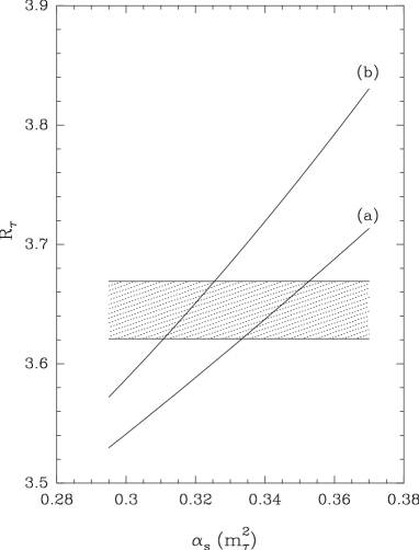
Figure 3: The Borel summation (15) of $R_{\tau}$, using the standard Taylor expansion $(a)$ and the improved expansion (30) $(b)$, as functions of $\alpha_{s}(m_{\tau}^{2})$. The band indicates the experimental values.

Using the experimental value [31]

$$(R_{\tau})_{exp}=3.645\pm 0.024\,,$$ (54)

we obtain

$$\alpha_{s}(m_{\tau}^{2})=0.343\pm(0.009)_{exp}\,,$$ (55)

using the standard Taylor expansion (11), and

$$\alpha_{s}(m_{\tau}^{2})=0.318\pm(0.007)_{exp}\,,$$ (56)

using the optimised expression (30). The improved expansion leads to a value of the coupling constant $\alpha_{s}(m_{\tau}^{2})$ lower by about 8% than the result given by the standard Taylor expansion of the Borel transform. Actually, as in the above discussion of the model functions at low $N$ and similar values of $\alpha_{s}$, the major contribution in shifting the value of $\alpha_{s}$ towards smaller values is brought by the explicit treatment of the first singularities of the Borel transform. At the small values of $\alpha_{s}$ relevant for the present problem, the effect of the conformal mapping is barely seen.

In (55) and (56) we indicated only the experimental error, which is very small. On the other hand, it is not easy to ascribe a definite theoretical error to these results. The problem of the theoretical error of $\alpha_{s}(m_{\tau}^{2})$ was discussed in many papers, in particular in [17], [23], [28]-[30], with different conclusions about its magnitude. One can safely neglect the effect of the uncertainties in the QCD parameters (quark masses, gluon condensate etc), which is small [27], [29] (leaving aside the still open problem of the $1/s$ corrections). The ambiguities related to the prescription chosen for computing the Laplace integral are believed to be small too, due to the conjecture that these ambiguities must be compensated by corresponding ambiguities in the condensates. The most important sources of theoretical error remain therefore those related to the analytic continuation from the euclidian to the minkowskian region, and the truncation of the perturbative expansion. A complete discussion of these errors is outside the objective of this paper. Concerning the analytic continuation, we only mention that in the derivation of (15) the perturbative expansion of the Adler function was assumed to be equally valid in the euclidian region and in the complex plane near the timelike axis, which is certainly not true. It is not trivial to relax this assumption and see its impact on the determination of $\alpha_{s}(m_{\tau}^{2})$. As concerns the truncation error, the estimate $\delta\alpha_{s}(m_{\tau}^{2})\simeq 0.05$ was suggested in [23] and [29], by comparing the predictions of different summation procedures. In [30] it was claimed on the other hand that much less errors are obtained if the renormalization group invariance of the perturbation series is exploited in an optimal way. The present work points towards a similar conclusion: indeed, as was remarked also in [17], it is rather arbitrary to interpret the spread of the results produced by different conformal mappings as a measure of the theoretical error, as suggested in [23]. Our investigation on mathematical models shows that the truncation error depends on the choice of the conformal mapping, being smaller if more information on the analyticity of the function is taken into account. The expansion proposed in our work exploits in an optimal way the (renormalization group invariant) information on the first renormalons of the Borel transform, and we therefore expect that the truncation error of the result (56) is smaller than the estimate given above.

4 Conclusions

The technique of the optimal conformal mapping of the Borel plane, discussed in this paper, can be seen as an alternative resummation of higher-order effects in perturbative QCD. This resummation method has a physical content in the sense that the requirement of convergence in powers of the optimal variable $w(u)$ amounts to a statement on analyticity in the whole double-cut Borel plane. Indeed, the theorem [22] on the asymptotic rate of convergence of power series, on which it is based, is dependent upon the condition that the function $f(u)$ (which is expanded) and the function $w(u)$ (in powers of which $f(u)$ is expanded, see (26)) should have the same location of singularities. The method of the optimal conformal mapping allows us to make full use of this analyticity property.

This remarkable feature is lost if the function is expanded in powers of some other variable, be it $u$ or a conformal mapping of $u$ such that only a part of the analyticity domain is mapped inside the convergence circle. In such cases, the convergence domain is smaller than the region of analyticity, and the requirement of convergence has to be supplemented with the analyticity condition. Only in the case of the optimal mapping the two regions are identical.

As renormalons express the properties of the Feynman diagrams of the process, a statement about their location implies a statement about the physics of the process considered.

If the power expansion is truncated at a definite order, as is the case in practice, the roles of $u$ and $w(u)$ are modified. While a polynomial in $u$ is holomorphic in $u$ and has no singularites in the Borel plane, a polynomial in $w$ has the same analyticity region as the expanded function, having the cuts equally located. Since singularities have physical interpretation, every polynomial in $w(u)$ carries this piece of information.

We demonstrated the practical use of the optimized expansion numerically on a large number of model functions, for a sufficiently large truncation order ($N\geq 5$). The accuracy of the Laplace integral is especially increased by the optimal variable if the coupling constant is large and the exponential damping of the integrand is weak. In these cases the knowledge (even approximate) of the behaviour near the first renormalons, combined with the expansion in the optimal variable, leads to very accurate results, while the expansion in the Borel variable, though partially improved by the treatment of the branch points, fails dramatically. On the other hand, at low orders of perturbation expansion and for values of the coupling constant of physical interest the effect of the optimal conformal mapping is not very visible and the predominant effect is given by the explicit treatment of the nearest branch points. This was actually the case with the determination of the strong coupling constant $\alpha_{s}(m_{\tau}^{2})$ from the hadronic $\tau$ decay width: the combined technique of conformal mapping and the explicit treatment of the first branch points of the Borel transform reduce by about 8% the value given by the usual Taylor expansion in the Borel variable. The major contribution to this result is brought by the theoretical information [10], [20] about the nature of the first renormalons.

Acknowledgements: We are grateful to Prof. A. de Rújula and the CERN Theory Division for hospitality while a part of this work was done. One of us (I.C.) thanks Prof. H. Leutwyler for his kind hospitality at the Institute of Theoretical Physics, University of Berne, and the Swiss National Science Foundation for support in the program CSR CEEC/ NIS, Contract No 7 IP 051219. The other author (J.F.) is indebted to Prof. G. Altarelli for reading the manuscript and stimulating discussions and remarks. The work was supported in part by GAAV and GACR (Czech Republic) under grant numbers A1010711 and 202/96/1616 respectively.

References

- [1] L.N.Lipatov, Sov.Phys. JETP 45, 216 (1977).
- [2] E.B. Bogomolny and V. A. Fateyev, Phys. Lett. 71B, 93 (1977).
- [3] B. Lautrup, Phys.Lett.B69,109 (1977).
- [4] G. Parisi, Phys. Lett.B76, 65 (1978).
- [5] J.J. Loeffel, Rep.Saclay DPh-T/76-20, unpublished.
- [6] J.C. Le Guillou and J.Zinn-Justin, Phys.Rev.Lett.39, 95 (1977).
- [7] N.N. Khuri, Phys. Rev. D16, 1754 (1977).
- [8] N.N. Khuri, Phys. Lett. 82B, 83 (1979).
- [9] G. ’t Hooft, in: The Whys of Subnuclear Physics, Proceedings of the 15th International School on Subnuclear Physics, Erice, Sicily, 1977, edited by A. Zichichi (Plenum Press, New York, 1979), p. 943.
- [10] A.H. Mueller, in ”QCD- Twenty Years Later”, Aachen 1992, eds. P. Zerwas and H.A. Kastrup, World Scientific, Singapore.
- [11] M. Beneke and V. I. Zakharov, Phys. Lett. B312 340 (1993).
- [12] D. Broadhurst, Z. Phys. C 58, 339 (1993).
- [13] M. Beneke, Phys. Lett. B 307, 154 (1993); Nucl. Phys. B 405, 424 (1993).
- [14] C. N. Lovett-Turner and C. J. Maxwell, Nucl. Phys. B452, 188 (1995).
- [15] M. Neubert, Phys. Rev. D 51, 5924 (1995).
- [16] Yu.L.Dokshitzer and N.G.Uraltsev, Phys.Lett. B380, 141 (1996).
- [17] P. Ball, M. Beneke and V.M. Braun, Nucl. Phys. B452, 563 (1995).
- [18] A. I. Vainshtein and V.I. Zakharov, Phys. Rev. Lett. 73 1207 (1994); Phys. Rev. D54 4039 (1996).
-
[19]
J. Fischer, Fortsch.Phys. 42, 665 (1994);
J. Fischer, Int. J.Mod.Phys. A 12, 3625 (1997). - [20] M. Beneke, V.M. Braun and N. Kivel, Phys. Lett. B 404, 315 (1997).
- [21] G.N. Hardy, Divergent Series, Oxford University Press, 1949.
- [22] S. Ciulli and J. Fischer, Nucl. Phys. 24, 465 (1961).
- [23] G. Altarelli, P. Nason and G. Ridolfi, Z. Phys. C 68, 257 (1995).
- [24] D.E. Soper and L. R. Surguladze, Phys. Rev. D 54, 4566 (1996).
- [25] J.Ellis, E. Gardi, M. Karliner and M.A. Samuel, Phys. Lett. B 366, 268 (1996); Phys.Rev. D 54, 6986 (1996).
- [26] S. Narison and A. Pich, Phys. Lett. 211, 183 (1988).
- [27] E. Braaten, S. Narison and A. Pich, Nucl. Phys. B 373, 581 (1992).
- [28] F. Le Diberder and A. Pich, Phys. Lett. B 286, 147 (1992).
- [29] M. Neubert, Nucl.Phys. B 463, 511 (1996).
- [30] C.J. Maxwell, Nucl.Phys.Proc.Suppl. 64, 360 (1998).
- [31] L.Duflot (Aleph Collaboration) Nucl.Phys. B (Proc.Suppl) 40, 37 (1995)
- [32] T. Coan et al (Cleo Collaboration) Phys.Lett. B 356, 580 (1995).
- [33] K.G. Chetyrkin, A.L. Kataev and F.V. Tkachov, Phys. Lett. B 85, 277 (1979).
- [34] M. Dine and J. Sapirstein, Phys. Rev. Lett. 43, 668 (1979).
- [35] W. Celmaster and R. Gonsalves, Phys. Rev. Lett. 44, 560 (1980).
- [36] S.G. Gorishny, A.L. Kataev and S.A. Larin, Phys. Lett. B 259, 144 (1991).
- [37] L.R. Surguladze and M.A. Samuel, Phys. Rev. Lett. 66, 560 (1991) [E: 66, 2416 (1991)].
- [38] I. Ciulli, S. Ciulli and J. Fischer, Nuovo Cim. 23, 1129 (1962).
- [39] Tables of Integral Transforms, Bateman Manuscript Project, Vol.I, ed. A. Erdélyi, McGraw-Hill, 1954, pag.134.
- [40] M. Abramowitz and I. Stegun, Handbook of mathematical functions, Dover Publ.,Inc. New York,1968.