Theory of Spin Effects in
Hard Hadronic Reactions

Abstract

I discuss the present situation with regard to a variety of theoretical topics in hadronic spin physics: (a) global analysis of the $g_{1}$ data—positivity at leading and next-to-leading order, renormalisation-scheme dependence, parametrisation, and hyperon $\beta$-decays; (b) items from the realm of transverse spin—twist-three effects, single-spin asymmetries, and transversity; and finally (c) recent developments in understanding the $Q^{2}$ evolution of orbital angular momentum.

1 Introduction

Let me begin by thanking the Local Organising Committee for kindly inviting me to attend the Symposium and for large amount the time and effort that went into making my arrival in Protvino at all possible. I should also like to take this opportunity to congratulate them for succeeding, notwithstanding the obvious difficulties, in attaining a balanced mix of informative and instructive talks from both experimentallists and theorists alike.

1.1 General Outline

Given the generously broad title assigned to me, I have attempted to at least touch upon those subjects not already covered by other plenary or parallel speakers. From the schedule, it emerged that the following areas were among those least represented in the theoretical talks (although some have been partially covered in the experimental presentations):

• global $g_{1}$ data analysis—renormalisation scheme dependence, positivity at LO and NLO, and hyperon $\beta$-decays;

• transverse spin—twist-three, single-spin asymmetries, transversity, and inequalities;

• orbital angular momentum—evolution and gauge dependence.

Thus, following a few introductory notes on factorisation formulæ and global spin sum rules, I shall endeavour to give a flavour of the present stage of development of the above topics. That said, the use and importance of inequalities in transverse-spin variables will only fully emerge as and when precise data become available. Moreover, the problem of gauge invariance in orbital angular momentum is particularly technical and perhaps of little phenomenological significance as yet. Therefore, while recently arousing increasing theoretical interest, these last two topics will not be covered here. Finally, to avoid unnecessary repetition, I shall omit detailed definitions wherever possible, which may be found in either earlier talks or the original literature.

1.2 Factorisation Formulæ

Schematically, the cross-section for the hadronic process $AB\to{}CX$ is

$$F_{A}(x_{A})\;\otimes\;F_{B}(x_{B})\;\otimes\;d\hat{\sigma}\;\otimes\;D_{C}(z_{C}),$$ (1)

where $F_{i}(x_{i})$ are partonic densities, $d\hat{\sigma}$ is the partonic hard-scattering cross-section, and $D_{i}(z_{i})$ is a fragmentation function. The symbols $\otimes$ represent convolutions in $x_{i}$ and $z_{i}$, the partonic longitudinal momentum fractions; and there is an implicit sum over parton flavours and types. Each term in the above expression has an expansion in both $\alpha_{s}$ and twist.

Cross-section (1) simplifies considerably in certain cases: e.g., when one or more of the partons is replaced by a photon (or weak boson), or if the final state is unobserved and is therefore to be summed over. It is also important to recall that spin does not represent an obstacle to the factorisation procedure nor to application of the above formula: the quantities relating to polarised particles are merely replaced by their spin-weighted counterparts (single-spin asymmetries are slightly more involved, requiring some form of angular weighting). It is instructive to recall the following aspects of the formula:

• radiative corrections induce logarithmic scale dependence in all factors (expressed via an $\alpha_{s}$ expansion);

• factorisation is carried out “twist-by-twist”;

• it is already more complicated at twist 3, in that diagrams naïvely higher-order in $\alpha_{s}$ can contribute even at leading order;

• twist-3 cross-sections are constructed with one and only one of the terms calculated at twist 3; the rest are calculated at twist 2, as usual.

The third point above is a common source of error: naïvely, one might expect twist-3 effects to be due only to explicitly higher-dimension terms, e.g., the quark mass. However, it is now known that the dominant twist-3 contributions come from diagrams with an extra partonic leg,[1] associated with an apparent extra power of $\alpha_{s}$. Moreover, relations involving twist-2 contributions require that the factor of $\alpha_{s}$ be absorbed into the correlation functions,[1] thus promoting such contributions to truly leading order in $\alpha_{s}$. Hence, the only suppression asymptotically is the typical $M/p_{T}$ associated with twist 3, which means that one might reasonably expect such effects to be large: e.g., even for $p_{T}\sim 10$ GeV (assuming the natural mass scale $M$ to be of the order of the nucleon mass) the asymmetries should be of order 10%.

A complication now emerging, with the realisation that large twist-3 single-spin asymmetries (SSA) may exist, is that there are many possible sources. At next-to-leading twist (i.e., three), all terms but one in the above factorisation product are taken at leading twist (two) and just one term at the next contributing twist (three). Thus, we are faced with the problem of isolating the true source among several possibilities, which might all turn out to contribute.

1.3 Global Sum Rules

Another important and intuitive decomposition is that of the $z$-axis projection of the total nucleon spin:

$$J_{z}^{p}=\frac{1}{2}=\frac{1}{2}\Delta\Sigma+\Delta g+L_{z}^{q+g},$$ (2)

together with the twin sum rule for the transverse projection:

$$J_{T}^{p}=\frac{1}{2}=\frac{1}{2}\Delta_{T}\Sigma+\Delta_{T}g+L_{T}^{q+g}.$$ (3)

I include the transverse-spin sum rule merely as a reminder of its existence. There are extra subtleties here: for example, the densities, $\Delta_{T}\Sigma$, have twist-3 contributions (absent for longitudinal polarisation).

Difficulties in the definitions of partonic densities are caused by both scheme and gauge dependence:

(i)i renormalisation ambiguities mix $\Delta\Sigma$ and $\Delta{g}$ at NLO;

(ii) the separation into spin and orbital components is gauge dependent.

To some extent, the problem of gauge dependence is circumvented by the natural axial-gauge choice in factorisation proofs and formulæ. However, the problem of identifying operators with meaningful physical quantities is fraught with ambiguity. Much attention has recently been paid to the orbital angular momentum case; [3] for lack of space the reader is referred to the literature.

2 Global $g_{1}$ data analysis

2.1 Positivity in Parton Densities

The experimental asymmetry is expressed (at leading twist) as

$$A_{1}\equiv\frac{\sigma_{1/2}-\sigma_{3/2}}{\sigma_{1/2}+\sigma_{3/2}}=\frac{g_{1}(x,Q^{2})}{F_{1}(x,Q^{2})}.$$ (4)

Thus, $g_{1}$ is bounded by $F_{1}$: $|g_{1}|{\leq}F_{1}$. Now, at the partonic level, $F_{1}$ and $g_{1}$ are defined in terms of sums and differences of helicity densities:

$$f=f^{\uparrow}+f^{\downarrow},\qquad\Delta f=f^{\uparrow}-f^{\downarrow}.$$ (5)

Therefore, the positivity of $f^{\uparrow,\downarrow}$ would lead to a useful bound:

$$|\Delta f(x,Q^{2})|\leq f(x,Q^{2}).$$ (6)

However, beyond LO there is no guarantee of positivity; even quark helicity flip is possible (via the ABJ axial anomaly).

In this respect, note that, in principle, even the un-polarised densities could become negative (owing to virtual corrections). Only in the naïve parton model (or LO) are the densities positive definite (by definition). At NLO, the ambiguities inherent in the choice of renormalisation scheme make negative densities possible in particular schemes. To understand this, recall that physical quantities correspond to partonic densities multiplied by coefficient functions (a power series in $\alpha_{s}$); beyond LO, partonic densities themselves should not be thought of as physically measurable quantities. In fact, positivity is partially rescued by the fact that if higher-order corrections became large enough to change the sign, perturbation theory would not be valid.

2.2 Positivity Beyond LO

Including the NLO corrections, the inequalities take on the following form (moment-by-moment but suppressing $N$ and $Q^{2}$ for clarity): [4, 5]

$$\frac{\left|\left(1+\frac{\alpha_{s}}{2\pi}\Delta C^{d}_{\Sigma}\right)\Delta\Sigma+\frac{\alpha_{s}}{2\pi}\Delta C^{d}_{g}\Delta g\right|}{\left(1+\frac{\alpha_{s}}{2\pi}C^{d}_{\Sigma}\right)\Sigma+\frac{\alpha_{s}}{2\pi}C^{d}_{g}g}\leq 1,$$ (7)

using DIS as the natural defining process for quark densities. And

$$\frac{\left|\left(1+\frac{\alpha_{s}}{2\pi}\Delta C^{h}_{g}\right)\Delta g+\frac{\alpha_{s}}{2\pi}\Delta C^{h}_{\Sigma}\Delta\Sigma\right|}{\left(1+\frac{\alpha_{s}}{2\pi}C^{h}_{g}\right)g+\frac{\alpha_{s}}{2\pi}C^{h}_{\Sigma}\Sigma}\leq 1,$$ (8)

using Higgs production as a possible defining process for the gluon density.[4, 5] This is actually a gedanken experiment, in which one imagines producing a Higgs particle via a gluon-proton collision. The bounds so derived are shown for two example moments in fig. 1. Such bounds may be useful to pin down the shape of $\Delta{g(x)}$, see fig. 2.

Figure 1: The LO (dashed lines) and NLO (solid lines) positivity bounds on $\Delta\Sigma(N)$ and $\Delta{g(N)}$ for $Q^{2}=1$ GeV² and $N=2$, 5, from Altarelli et al.[4]

Figure 2: The maximal gluon density at $Q^{2}=1$ GeV² obtained from LO (dashed lines) and NLO (solid lines) positivity bounds, using polarized quark densities from two fits of Altarelli et al.[6] The corresponding best-fit polarized gluon density is also shown (dot-dashed).

At present, $\Delta{g(x)}$ is essentially determined via scaling violations alone, which fix only the low moments with any precision, since $|\gamma_{qg}|\ll|\gamma_{qq}|$ for large $N$ (see fig. 3):

Figure 3: The LO anomalous dimensions $\gamma_{qq}(N)$ and $\gamma_{qg}(N)$ (respectively, the top and bottom curves at small $N$) as a function of $N$, from Forte et al.[5]

$$\frac{d}{dt}\,g_{1}^{\rm singlet}=\frac{\langle e^{2}\rangle}{2}\frac{\alpha_{s}}{2\pi}\left[\rule[0.0pt]{0.0pt}{8.61108pt}\gamma_{qq}\Delta\Sigma+2n_{f}\gamma_{qg}\Delta g\right]+\mathrm{O}(\alpha_{s}^{2}).$$ (9)

2.3 More on Positivity

Analysis of the evolution of individual spin components shows the problem to be partially “self-curing”; [7] at LO the IR-singular terms (with the usual $+$ prescription) lead to

$$\frac{dq(x)}{dt}=\frac{\alpha_{s}}{2\pi}\left[\int_{x}^{1}dy\frac{q(y)}{y}P\left(\frac{x}{y}\right)-q(x)\int_{0}^{1}dzP(z)\right].$$ (10)

The second term cannot change the sign of $q(x)$ as it is diagonal in $x$: as $q(x)$ approaches zero, so too does the very term driving it toward the sign change. Full $q$-$g$ mixing leads to (for example)

$$\frac{dq_{+}(x)}{dt} = \frac{\alpha_{s}}{2\pi}\left[P_{++}^{qq}\left(\frac{x}{y}\right)\otimes q_{+}(y)+P_{+-}^{qq}\left(\frac{x}{y}\right)\otimes q_{-}(y)\right.$$ (11)

$$\quad\left.+P_{++}^{qg}\left(\frac{x}{y}\right)\otimes g_{+}(y)+P_{+-}^{qg}\left(\frac{x}{y}\right)\otimes g_{-}(y)\right].$$

Again, the only singular terms in this and the three companion equations are diagonal (in parton type too) and therefore cannot spoil positivity.

The result survives to NLO order,[7] except for a small violation in the $qg$ and $gq$ kernels at $x\sim 0.7$, which, it is conjectured, might be cured by an appropriate choice of $\gamma_{5}$ scheme. Thus, positivity may be a useful addition to the data fitters’ armoury. However, care is required to avoid those schemes in which it could cause undesirable bias in fit results.

2.4 Renormalisation Scheme Choice

In order to analyse data, a certain amount of theoretical input is necessary. Thus, there are several other issues (some of which are apparently exquisitely theoretical) requiring careful examination since they can in fact have a significant impact on the outcome of global data fits involving parton evolution:

• definition of polarised gluon and singlet-quark densities,

• small-$x$ extrapolation,

• choice of initial parametrisation.

Though mathematically acceptable, a peculiarity of the $\overline{\rm MS}$ scheme is that some soft contributions are included in the Wilson coefficient functions, rather than being absorbed into the parton densities. Consequently, the first moment of $\Delta\Sigma$ is not conserved and it is difficult to compare the DIS results on $\Delta\Sigma$ with constituent quark models at low $Q^{2}$. To avoid such oddities, Ball et al.[8] have introduced the so-called Adler-Bardeen (AB) scheme, now a common choice. The AB scheme involves a minimal modification of the $\overline{\rm MS}$ scheme; the polarised singlet quark density is fixed to be scale independent at one loop:

$$a_{0}(Q^{2})\;=\;\Delta\Sigma\,-\,n_{f}\frac{\alpha_{s}(Q^{2})}{2\pi}\,\Delta g(Q^{2}).$$ (12)

Other factorisation schemes will not alter $\Delta{g(Q^{2})}$ greatly but may, in contrast, cause $\Delta\Sigma$ to vary considerably. As a result, the values of $a_{0}(\infty)$ and $\Delta\Sigma$ will be very different. Recall that $\Delta{g(Q^{2})}$ grows as $1/\alpha_{s}(Q^{2})$. Of course, the difference between any two schemes lies in the (unknown) higher-order terms. Thus, comparison of results between two schemes (e.g., AB and $\overline{\rm MS}$) could also shed light on the importance of the NNLO corrections.

Zijlstra and van Neerven [10] have pointed out that the AB scheme described above is just one of a family of schemes keeping $\Delta{q_{NS}}$ scale independent.

$$\pmatrix{\Delta\Sigma\cr\Delta g}_{a}=\pmatrix{\Delta\Sigma\cr\Delta g}_{\overline{\rm MS}}+\frac{\alpha_{s}}{2\pi}\pmatrix{0&z(x;a)_{qg}\cr 0&0}\otimes\pmatrix{\Delta\Sigma\cr\Delta g}_{\overline{\rm MS}},$$ (13)

where $z_{qg}(x;a)=N_{f}[(2x-1)(a-1)+2(1-x)]$. The AB scheme corresponds to $a=2$; Leader et al.[9] propose yet another scheme they call the JET scheme, in which $a=1$. In this scheme all hard effects are absorbed into the coefficient functions and the gluon coefficient is as it appears in $pp{\to}JJ+X$.

The transformation between the $\overline{\rm MS}$ and JET schemes is then given by the following (suppressing the $Q^{2}$ dependence):

$$\Delta\Sigma^{(n)}_{\rm JET} = \Delta\Sigma^{(n)}_{\overline{\rm MS}}+\frac{n_{f}\alpha_{s}}{2\pi}\frac{2}{n(n+1)}\Delta g^{(n)}_{\overline{\rm MS}},$$ (14)

$$\Delta g^{(n)}_{\rm JET} = \Delta g^{(n)}_{\overline{\rm MS}}.$$ (15)

For example, such a transformation indicates that the polarised strange sea, $\Delta{s}$, will be different in the two schemes. Of course, AB and JET are the same for $n=1$. The analogous transformation of the coefficient functions and anomalous dimensions from the $\overline{\rm MS}$ to the AB scheme is given by replacing the factor $2/n(n+1)$ with $1/n$. Thus, the ABJ anomaly, far from being an obstacle, may provide a route to parton definitions of a physically intuitive and meaningful form.

2.5 Small-$x$ Extrapolation

The main problem with regard to parametrisation is the extrapolation $x{\to}0$. As shown by De Rújula [11] and later studied by Ball and Forte,[12] PQCD evolution leads to the following un-polarised small-$x$ asymptotic behaviour:

$$g \sim x^{-1}\sigma^{-1/2}e^{2\gamma\sigma-\delta\zeta}\left(1+\sum_{i=1}^{n}\epsilon^{i}\rho^{i+1}\alpha_{s}^{i}\right)$$ (16)

$$\Sigma \sim x^{-1}\rho^{-1}\sigma^{-1/2}e^{2\gamma\sigma-\delta\zeta}\left(1+\sum_{i=1}^{n}\epsilon_{f}^{i}\rho^{i+1}\alpha_{s}^{i}\right),$$ (17)

$\xi=\log{x_{0}/x}$, $\zeta=\log{\left(\alpha_{s}(Q_{0}^{2})/\alpha_{s}(Q^{2})\right)}$, $\sigma=\sqrt{\xi\zeta}$, $\rho=\sqrt{\xi/\zeta}$, and the $\epsilon^{i}$ terms indicate $i$-th order corrections. In the un-polarised case, the leading singularity is carried by gluons, which drive the singlet quark evolution. However, all polarised singlet anomalous dimensions are singular and therefore gluons and quarks “mix”. Moreover, the asymptotic predictions hold only for non-singular input densities: a singular starting point is preserved. It follows that the structure functions $xF_{1}$ and $F_{2}$ rise at small $x$ more and more steeply as $Q^{2}$ increases, though, for all finite $n$, never as steeply as a power of $x$.

All other parton densities $f$ ($f=q_{NS}$, $\Delta q_{NS}$, $\Delta\Sigma$, $\Delta g$) behave as

$$f\sim\sigma^{-1/2}e^{2\gamma_{f}\sigma-\delta_{f}\zeta}\left(1+\mbox{$\sum_{i=1}^{n}$}\epsilon_{f}^{i}\rho^{2i+1}\alpha_{s}^{i}\right).$$ (18)

These last are less singular than the unpolarized singlet densities by a power of $x$, while the higher-order corrections are more important at small $x$ since the exponent $i+1$ is replaced by $2i+1$; because the leading small $N$ contributions to the anomalous dimensions at order $\alpha_{s}^{i+1}$ are $\left(\alpha_{s}/(N-1)\right)^{i}$ in the unpolarized singlet case, but $N\left(\alpha_{s}/N^{2}\right)^{i}$ for the non-singlet and polarized densities. Altarelli et al. obtain better fits using a logarithmic form (rather than a power). Although this is reminiscent of evolution effects and is compatible with Regge theory too, no conclusions can be drawn from such results. As a final comment, fits generally give good overall agreement with PQCD evolution.

2.6 Input Sea Symmetry Assumptions

To fit data, assumptions for the sea polarisation are usually necessary; a common choice is flavour symmetry: $\Delta\bar{s}=\Delta\bar{u}=\Delta\bar{d}$. To test such a hypothesis, Leader et al.[9] note that if one allows $\Delta\bar{s}=\Delta\bar{u}=\lambda\Delta\bar{d}$, then the data (via $\beta$-decay couplings) fix $\Delta{q_{3,8}}$, $\Delta\Sigma$ and $\Delta{G}$. Thus, while

$$\Delta\bar{s}=\frac{1}{6}(\Delta\Sigma-\Delta q_{8}),$$ (19)

and therefore $\Delta\bar{s}$ clearly does not vary with $\lambda$.

On the other hand,

$$\Delta u_{v} = \frac{1}{2}[\hphantom{-}\Delta q_{3}+\Delta q_{8}-4(\lambda-1)\Delta\bar{s}],$$ (20)

$$\Delta d_{v} = \frac{1}{2}[-\Delta q_{3}+\Delta q_{8}-4(\lambda-1)\Delta\bar{s}],$$ (21)

so, valence densities are sensitive to sea assumptions. However, the dependence on $\lambda$ can only arise via scaling violation and hence is weak, as seen in the analysis (indeed, it is likely an artifact). Results for $\Delta\bar{s}$ should not change significantly as the input value of $\lambda$ varies, thus testing the analysis stability.

2.7 Input Non-Singlet Shape Assumptions

In order to reduce the number of free parameters in the fitting procedure, a further assumption sometimes adopted is

$$\Delta q_{3}(x,Q^{2})\propto\Delta q_{8}(x,Q^{2}).$$ (22)

While compatible with evolution (both are non-singlet densities), it cannot be at all justified as a starting point: allowing the two densities, $\Delta q_{3}(x,Q^{2})$ and $\Delta q_{8}(x,Q^{2})$, to vary independently, significant differences are found,[9] see fig. 4 (recall the $u(x)-d(x)$ difference). Thus, such an assumption will certainly distort parameter values and errors obtained. Note too that the data do indeed constrain valence densities well.

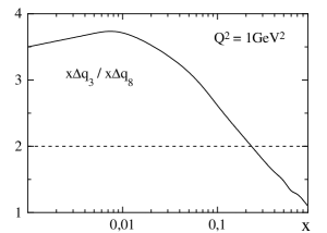
Figure 4: The ratio $\Delta{q_{3}(x,Q^{2})}/\Delta{q_{8}(x,Q^{2})}$, from Leader et al.[9]

2.8 Hyperon Data Input

Together with the Bjorken sum-rule input, $a_{3}=F+D$, the “hypercharge” equivalent, $a_{8}=3F-D$, is also needed. The measured baryon-octet $\beta$-decays can provide the extra information: assuming SU$(3)_{f}$ symmetry, all hyperon semi-leptonic decays (HSD) may be described moderately well in terms of the Cabibbo mixing angle and precisely the two parameters required, $F$ and $D$. The precision of the HSD data is better than presently needed for DIS analyses. However, since SU(3) violation is typically of order 10%, one worries that the extracted values of the two parameters could suffer the same order of shift.

There exist SU(3)-breaking analyses returning $F/D\simeq 0.5$ (cf. the standard value: 0.58), but the poor $\chi^{2}$ of all such fits casts doubt on their validity. Pure SU(3) fits to the hyperon semi-leptonic decays are also often used. These typically return $F/D\simeq 0.575$, but again the fits are very poor: $\chi^{2}\simeq 2/$DoF. On the other hand, SU(3) breaking fits with only one new parameter, give much better agreement: $\chi^{2}\simeq 1/$DoF.[13] These fits return $F/D\simeq 0.57$, which is also stable with respect to the SU(3) breaking approach adopted.

3 Tests of Perturbation Theory

One of the many ways to test PQCD is to compare $\alpha_{s}$ as extracted in different processes. A particularly suggestive method used of late is to show the order-by-order agreement in, e.g., the Bjorken sum-rule (see fig. 5). While data are unambiguous, modulo the usual experimental uncertainties, such a plot is misleading from a theoretical viewpoint: as commented from the floor at this symposium, the naïve interpretation would not be convergence of the perturbation series to the correct value, rather an imminent crossing and possible premature divergence. Although PQCD perturbation series are generally held to be asymptotic, this is clearly not what is being displayed here.

The problem lies in the use of a fixed-order $\alpha_{s}$: it is simply incorrect to use a fixed-order extraction of $\alpha_{s}$ in variable-order predictions. In the majority of cases the perturbative expansion displays monotonic behaviour (at least for the few known terms), just as the Bjorken series. Hence, as the order of perturbation theory used for extraction increases, the value of $\alpha_{s}$ obtained decreases. Thus, taking the world mean $\alpha_{s}$ to be (on average) second order, a first-order extraction would provide a relatively larger value and third and fourth orders, progressively smaller. Correct order-by-order comparison would then lead to the shifts indicated in fig. 5 and therefore milder convergence.

Figure 5: The order-by-order comparison of data and theory for the Bjorken sum-rule: the data points are corrected for QCD and the dashed line is $g_{A}/g_{V}$. The arrows indicate the directions and relative magnitudes of the shifts indicated in the text.

4 Transverse Polarisation

Transverse spin has many facets, I now turn to the status of PQCD approaches to the long-standing puzzle of single-spin asymmetries and also mention some recent developments in transversity. Inequalities are important here too, as constraints on model builders’ input densities for predictive purposes [14] but again, being technical in nature, I shall not discuss them further.

4.1 Single-Spin Asymmetries

A most interesting aspect of transverse spin is the large amount of SSA data: measured effects reach the level of 40–50% in a wide range of processes.[15] Ever since Kane et al.,[16] it has been realised that at twist 2 in LO massless PQCD such effects are zero. At NLO, the effects due to imaginary parts of loop diagrams are found to be at most of order 1%.

However, since the pioneering work of Efremov and Teryaev,[2] it is now well understood that twist-3 effects naturally lead to such asymmetries. To calculate the SSA in prompt-photon production Qiu and Sterman [17] have exploited their idea of taking the necessary imaginary part from soft propagator poles arising in extra partonic legs inherent to twist-3 contributions. Since then Efremov et al.[18] have performed calculations for the pion asymmetry, as too have Qiu and Sterman,[19] and Ji [20] has examined the purely gluonic contributions. The results are all very encouraging.

4.2 Factorisation in Higher-Twist Amplitudes

A difficulty in such calculations is the large number (several tens) of PQCD diagrams encountered. Recently I have shown [21] that, in the pole limit of interest, the contributions simplify owing to a factorisation of the soft insertion from the rest of the amplitude, see fig. 6.

Figure 6: Representation of the amplitude factorisation in the case of a soft external gluon line $x_{g}{\to}0$. The solid circle indicates the propagator from which the imaginary piece is extracted, and $\xi$ is the polarisation vector of the gluon entering the factorised vertex.

The remaining $2{\to}2$ helicity amplitudes are known; thus, calculation of any such process reduces to simple products of known helicity amplitudes with the above “insertion” factors (including modified colour factors). The factorisation described, also leads to more transparent expressions clarifying why large SSA’s may be expected: there is no reason for suppression (kinematic mismatch etc.), beyond their higher-twist nature.

4.3 Unravelling Higher Twist in Single Spin Asymmetries

A complication that has emerged is that the possible mechanisms for producing such asymmetries are numerous (even when restricted to the purely PQCD processes described, not to mention the problem of intrinsic $k_{T}$ [22]). Thus, it is now important to analyse the possible processes in which SSA’s are allowed and to identify those with differing origins, in the hope of eliminating some candidates and finally arriving at the true source. A step in this direction has been taken by Boros et al.,[23] see table 1, and an interesting discussion has also been presented at this symposium by Murgia.[22]

Table 1: Predictions for other SSA’s under different hypotheses for the origins of the pion asymmetry, from Boros et al.[23]

	if $A_{N}$ observed in $p(\uparrow)+p\to\pi+X$ originates from …
process	quark distribution function	elementary scattering process	quark fragmentation function	orbital motion and surface effect
$l+p(\uparrow)\to l+\left(\begin{array}[]{c}\pi^{\pm}\\ K^{+}\end{array}\right)+X$	$A_{N}=0$ wrt jet axis	$A_{N}=0$ wrt jet axis	$A_{N}\neq 0$ wrt jet axis	$A_{N}=0$ wrt jet axis
current fragmentation region for large $Q^{2}$ and large $x_{B}$	$A_{N}\neq 0$ wrt $\gamma^{\star}$ axis	$A_{N}=0$ wrt $\gamma^{\star}$ axis	$A_{N}\neq 0$ wrt $\gamma^{\star}$ axis	$A_{N}=0$ wrt $\gamma^{\star}$ axis
$l+p(\uparrow)\to l+\left(\begin{array}[]{c}\pi^{\pm}\\ K^{+}\end{array}\right)+X$ target fragmentation region for large $Q^{2}$ and large $x_{B}$	$A_{N}\neq 0$	$A_{N}=0$	$A_{N}\neq 0$	$A_{N}=0$
$p+p(\uparrow)\to\left(\begin{array}[]{c}l\bar{l}\\ W^{\pm}\end{array}\right)+X$ $p(\uparrow)$ fragmentation region	$A_{N}\neq 0$	$A_{N}\approx 0$	$A_{N}=0$	$A_{N}\neq 0$

4.4 Transversity

Despite the advantage of being twist-2 and therefore unsuppressed, transversity cannot contribute to inclusive DIS as it requires quark helicity flip. However, Jaffe et al.[24] have recently proposed its measurement via twist-two quark-interference fragmentation functions, see fig. 7.

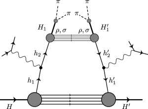
Figure 7: Diagram for double-pion production via $\sigma$, $\rho$ in DIS.

This is remeniscent of the so-called handedness property but appears more direct to interpret.

FSI between, e.g., $\pi^{+}\pi^{-}$, $K\overline{K}$, or $\pi{}K$, produced in the current fragmentation region in DIS on a transversely polarised nucleon may probe transversity. The point is that the pions may be produced through intermediate resonant states: $\sigma[(\pi\pi)^{I=0}_{l=0}]$ and $\rho[(\pi\pi)^{I=1}_{l=1}]$ produced in the current fragmentation region. Two new interference fragmentation functions can then be defined: $\hat{q_{I}}$, $\delta\hat{q_{I}}$; the subscript $I$ stands for interference. The final asymmetry, requiring no model input, has the following form: [24]

$${\cal A}_{\bot\top}\equiv\frac{d\sigma_{\bot}-d\sigma_{\top}}{d\sigma_{\bot}+d\sigma_{\top}} = -\frac{\pi}{4}\frac{\sqrt{6}(1-y)}{[1+(1-y)^{2}]}\cos\phi\sin\delta_{0}\sin\delta_{1}\sin\left(\delta_{0}-\delta_{1}\right)$$ (23)

$$\hskip 4.30554pt\times\;\frac{\sum_{a}e_{a}^{2}\delta q^{a}(x)\,\delta\hat{q}_{I}^{a}(z)}{\sum_{a}e^{2}_{a}q_{a}(x)\left[\sin^{2}\delta_{0}\hat{q}_{0}^{a}(z)+\sin^{2}\delta_{1}\hat{q}_{1}^{a}(z)\right]},$$

where $\hat{q}_{0}$ and $\hat{q}_{1}$ are spin-averaged fragmentation functions for the intermediate $\sigma$ and $\rho$ states, respectively.

Note that the target only need be polarised; the asymmetry is obtained either by flipping the nucleon spin or via the azimuthal asymmetry. This approach can also be extended to generate a (double) helicity asymmetry, which could probe valence-quark spin densities.[25]

5 Orbital Angular Momentum

It has long been well understood that angular-momentum conservation in parton splitting processes implies non-trivial $Q^{2}$ evolution of partonic orbital angular momentum (OAM),[26] in line with that of the gluon spin. Ji et al.[27] have shown that this leads to asymptotic sharing of total angular momentum identical to that of the linear momentum fraction. Recently, Teryaev [28] has rederived the PQCD evolution equations for OAM in a semi-classical approach in terms of the spin-averaged and spin-dependent kernels.

Generation of OAM, balancing the gluon spin, accompanies $q{\to}qg$ splitting. The net effect is obtained subtracting the probabilities of a gluon with negative and positive helicities. The same combination (modulo sign) appears in the $gq$ spin-dependent kernel, with momentum fraction $1{-}x$:

$$P^{LS}_{qq}(x)+P^{LS}_{gq}(1-x)=-\Delta P_{gq}(1-x).$$ (24)

The trick is that the ratio of the quark and gluon OAM can be found via classical reasoning. Before splitting, suppose the quark momentum has only a $z$ component, the final parton momenta are in the $x$-$z$ plane. By momentum conservation, the $x$ components of $q$ and $g$ momenta are equal (up to a sign) and the $z$ components of OAM are thus

$$L_{z}^{q}=P_{x}r^{q}_{y},\qquad L_{z}^{g}=-P_{x}r^{g}_{y},$$ (25)

where the spatial non-locality of quark and gluon production, $r^{q,g}$, has been introduced. OAM $x$ components are also generated:

$$L_{x}^{q}=-P^{q}_{z}r^{q}_{y},\qquad L_{x}^{g}=-P^{g}_{z}r^{g}_{y}.$$ (26)

Conservation of the $x$ component of OAM, $L_{x}^{q}=-L_{x}^{g}$, leads to

$$\frac{r^{q}_{y}}{r^{g}_{y}}=-\frac{P_{z}^{g}}{P_{z}^{q}},$$ (27)

and substitution into the $L_{z}$ eq. finally gives the partition:

$$\frac{L_{z}^{q}}{L_{z}^{g}}=\frac{P_{z}^{g}}{P_{z}^{q}}=\frac{1-x}{x},$$ (28)

precisely as Ji et al.[27] found by explicit calculation. Notice also that the whole problem of defining the relevant operators has been neatly circumvented.

6 Conclusions

In conclusion then, all theoretical aspects of spin physics continue to benefit from interest and study. Moreover, the rewards for the effort put into this sector are an ever-deeper understanding of hadronic structure (and may indeed represent one of the few real keys) while the various phenomenological puzzles are steadily coming under control.

Areas where there is more to be learnt are transverse spin (including transversity) and orbital angular momentum. The former, being linked to hadronic mass scales may provide important clues to the nature of chiral-symmetry breaking while there is also still much to explain of the known phenomenology, and transversity may yet have a rôle in single-spin asymmetries. OAM is as intriguing as it is elusive experimentally; its contribution the proton spin is yet to be measured and, were it to be found large, one would like to understand the implications for the standard SU(6) picture of the nucleon.

References

References

-
[1]
E.V. Shuryak and A.I. Vainshtein, Nucl. Phys.
B 201, 141 (1982);
A.V. Efremov and O.V. Teryaev, Sov. J. Nucl. Phys. 39, 962 (1984);
P.G. Ratcliffe, Nucl. Phys. B 264, 493 (1986). - [2] A.V. Efremov and O.V. Teryaev, Phys. Lett. B 150, 383 (1985).
-
[3]
X. Ji, Phys. Rev. Lett. 78, 610
(1997);
P. Hoodbhoy, X. Ji and W. Lu, e-prints hep-ph/9804337; 9808305;
D. Singleton and V. Dzhunushaliev, e-print hep-ph/9807239;
S.V. Bashinskii and R.L. Jaffe, e-print hep-ph/9804397. - [4] G. Altarelli, R.D. Ball, S. Forte and G. Ridolfi, Acta Phys. Pol. B 29, 1145 (1998).
- [5] S. Forte, G. Altarelli and G. Ridolfi, e-print hep-ph/9808462.
- [6] G. Altarelli, R.D. Ball, S. Forte and G. Ridolfi, Nucl. Phys. B 496, 337 (1997).
- [7] C. Bourrely, E. Leader and O.V. Teryaev, in the proc. of VII Workshop on High Energy Spin Physics (Dubna, Jul. 1997), to appear.
- [8] R.D. Ball, S. Forte and G. Ridolfi, Phys. Lett. B 378, 255 (1996).
- [9] E. Leader, A.V. Sidorov and D.B. Stamenov, e-prints hep-ph/9807251; 9808248.
- [10] E.B. Zijlstra and W.L. van Neerven, Nucl. Phys. B 417, 61 (1994); erratum ibid. B 426, 245 (1994).
- [11] A. De Rújula, Phys. Rev. 10, 1649 (1974).
- [12] R.D. Ball and S. Forte, Phys. Lett. B 335, 77 (1994); 336, 77 (1994); Acta Phys. Pol. B 26, 2097 (1995).
- [13] P.G. Ratcliffe, Phys. Lett. B 242, 271 (1990); 365, 383 (1996); e-print hep-ph/9806381, Phys. Rev. D, to appear.
-
[14]
O.V. Teryaev, e-prints hep-ph/9803403; 9808335;
D. de Florian, J. Soffer, M. Stratmann and W. Vogelsang, e-print hep-ph/9806513. - [15] A. Bravar, in these proceedings.
- [16] G.L. Kane, J. Pumplin and W. Repko, Phys. Rev. Lett. 41, 1689 (1978).
- [17] J. Qiu and G. Sterman, Phys. Rev. Lett. 67, 2264 (1991).
- [18] A.V. Efremov, V.M. Korotkiyan and O.V. Teryaev, Phys. Lett. B 348, 577 (1995).
- [19] J. Qiu and G. Sterman, e-print hep-ph/9806356.
- [20] X. Ji, Phys. Lett. B 289, 137 (1992).
- [21] P.G. Ratcliffe, e-print hep-ph/9806369.
- [22] F. Murgia, in these proceedings.
- [23] C. Boros, L. Zuo-tang, M. Ta-chung and R. Rittel, in the proc. of The XII Int. Symp. on High Energy Spin Physics (Amsterdam, Sept. 1996), eds. C.W. de Jager, T.J. Ketel, P.J. Mulders, J.E.J. Oberski and M. Oskam-Tamboezer (World Sci., 1997), p. 419; J. Phys. G 24, 75 (1998).
- [24] R.L. Jaffe, X. Jin and J. Tang, Phys. Rev. Lett. 80, 1166 (1998).
- [25] R.L. Jaffe, X. Jin and J. Tang, Phys. Rev. D 57, 5920 (1998).
- [26] P.G. Ratcliffe, Phys. Lett. B 192, 180 (1987).
- [27] X. Ji, X.J. Tang and P. Hoodbhoy, Phys. Rev. Lett. 76, 740 (1996).
- [28] O.V. Teryaev, B. Pire and J. Soffer, e-print hep-ph/9806502.