BUTP-98/26

hep-ph/9811342

COMPLETELY AUTOMATED CALCULATIONS OF MULTI-LOOP DIAGRAMS

The computation of higher order processes very often involves a large number of diagrams. In addition, it is in general not possible to solve the occurring integrals explicitly and expansions in small quantities have to be performed. This makes it necessary to automate the calculations as much as possible. A program package will be described which generates automatically the Feynman diagrams, manipulates the expressions in the desired way and performs the computation. As a physical application ${\cal O}(\alpha\alpha_{s})$ corrections to the decay rate of the $Z$ boson into bottom quarks are discussed.

1 Introduction and motivation

The impressive experimental precision reached so far mainly at LEP, SLC and TEVATRON has made it necessary to increase also the effort from the theoretical side. A crucial role plays thereby the computation of multi-loop diagrams in order to evaluate quantum corrections to the different observables.

Higher order corrections are mostly accompanied with a large number of diagrams. Very often it is a tedious job to do the bookkeeping and not to forget some relevant contributions. Especially when the number exceeds the order of a few hundred the generation should be passed to the computer. A further major task is the computation of the integrals. In most cases an exact solution is by far not possible and one has to rely on approximations. One possibility it to compute the integrals (at least partly) numerically. Another promising attempt is the use of asymptotic expansions which is applicable as soon as a certain hierarchy exist between the mass scales involved in the process. Well-defined prescriptions provide rules which specify the actions on the individual diagrams. In general each diagram generates several subgraphs which further increase the complexity of the calculation. Thus it is desired to automate the asymptotic expansion procedures. Of course, also the very computation of the single terms needs to be done by the computer as the size of intermediate expression become rather large.

In the next section a possible solution to the problems addressed above is presented by means of the package GEFICOM. In Section 3 its application to the computation of ${\cal O}(\alpha\alpha_{s})$ corrections to the decay of the $Z$ boson into bottom quarks is discussed.

2 GEFICOM: A package for generation and computation of Feynman diagrams

The automation of the computation of Feynman diagrams can be divided into different steps. In this section we will discuss them on the example of GEFICOM $\!{}^{{\bf?}}$. A flowchart is pictured in Fig. 1.

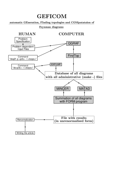
Figure 1: The structure of GEFICOM.

The user has to provide a few simple files specifying, e.g., the process, the particle content and the allowed vertices. Then, in a first step, the graphs contributing to the considered process have to be generated where the amplitudes at least need to contain information about the involved particles and the momenta flowing through each propagator. Inside GEFICOM the FORTRAN program QGRAF $\!{}^{{\bf?}}$ is used which has the advantage of being quite fast. Moreover different output formats are available one of which contains all the desired information on the diagrams.

The Feynman diagrams are classified according to their topology which becomes especially important during the calculation of the integrals. This information is, however, not provided by QGRAF and has to be determined from its output. For a human being this would be very easy. For a computer, on the other side, this is a quite non-trivial task and the momentum distribution has to be used in a clever way in order to extract the topology. This is done by FindTop which is part of a Mathematica program essentially inserting the Feynman rules and transforming the QGRAF output into FORM $\!{}^{{\bf?}}$ notation. Additionally administrative files are generated which rule the computation, sum up the diagrams etc. One finally ends up with a huge database containing all relevant files.

The very computation of the diagrams has to be initiated by the user. It is based on two FORM packages, MINCER $\!{}^{{\bf?}}$ and MATAD $\!{}^{{\bf?}}$, being able to deal with massless two-point, respectively, massive bubble diagrams up to three loops. Before, however, the amplitudes are passed to these packages there is the possibility to apply asymptotic expansions namely the hard-mass and large-momentum procedure providing consistent prescriptions on how to get expansions for large internal masses, respectively, large external momenta. They work on a diagram-by-diagram basis and make well-defined rules available which determine the subgraphs to be extracted from the original diagram $\!{}^{{\bf?}}$. The subgraphs have to be expanded in their small quantities before any momentum integration is performed. Thus significant simplifications are obtained and very often the integrals can be written as products of lower order ones at the price of — sometimes significantly — increasing their number. The automation of these procedures has been performed in the packages LMP $\!{}^{{\bf?}}$ and EXP $\!{}^{{\bf?}}$. They apply the asymptotic-expansion procedures and express the initial diagram as products of single-scale integrals which can be treated by MINCER and MATAD.

A very powerful tool for the computation of the diagrams is implemented into MINCER and MATAD, the so-called integration-by-parts technique. Up to now it has been systematically applied up to the three-loop level $\!{}^{{\bf?},{\bf?},{\bf?}}$. The general idea is quite simple: The integration-by-parts method exploits the fact that the momentum integrals in $D$ dimensions are finite. Thus the surface terms are zero:

$$\int{\rm d}^{D}p{\partial\over\partial p^{\mu}}f(p,\ldots) = 0\,.$$ (1)

The function $f$ in general is a product of scalar propagators belonging to the considered loop. Performing the derivatives in Eq. (1) explicitly leads to a sum of several terms which has to vanish identically. Combining different equations of this type, which are obtained by varying $f(p,\ldots)$ and choosing different loop momenta, leads to relations — so-called recurrence relations — where a complicated integral is expressed as a sum of simpler ones. The repeated application of recurrence relations finally leads to a sum simple integrals, which can be reduced to integrals of lower loop order, and only a few, so-called, master integrals which require a hard calculation.

At the three-loop level the described strategy has first been applied to massless two-point integrals $\!{}^{{\bf?}}$ and has later on been extended to massive bubble diagrams $\!{}^{{\bf?}}$. Also the corresponding master integrals are available $\!{}^{{\bf?}}$. These two sets of recurrence relations were implemented into MINCER and MATAD, respectively, and we will see in the next section that they provide when combined with the asymptotic expansions mentioned above a very powerful tool with a large field of application.

3 Application

The properties of the $Z$ boson have been measured to a very high accuracy — sometimes even at the permille level. Also the hadronic width of the $Z$ boson, $\Gamma_{\rm had}$, is known to an accuracy of roughly $0.1$%. An important contribution to $\Gamma_{\rm had}$ is provided by the partial rate into bottom quarks as already at one-loop order the top quark enters as a virtual particle giving rise to enhanced corrections proportional to $G_{F}M_{t}^{2}$. The full electroweak corrections are known since quite some time $\!{}^{{\bf?},{\bf?}}$ and also the leading terms of ${\cal O}(\alpha_{s}G_{F}M_{t}^{2})$ $\!{}^{{\bf?}}$ and ${\cal O}(\alpha\alpha_{s}\ln M_{t}^{2}/M_{W}^{2})$ $\!{}^{{\bf?}}$ are available since already a few years. Actually it turned out that the logarithmic contribution is relatively large as compared to the term quadratic in $M_{t}$ although $\ln(M_{t}^{2}/M_{W}^{2})$ is by far less enhanced than $M_{t}^{2}/M_{W}^{2}$. Thus the question arises whether the $M_{t}$-independent coefficient and the power-suppressed terms in the expansion lead to a significant change in the numerical prediction.

In the approach chosen in $\!{}^{{\bf?}}$ the $Z$ boson propagator was considered whose imaginary part directly leads to the decay width. The diagrams contributing at the two-loop level are shown in Fig. 2. A gluon has to be added in all possible ways in order to obtain the graphs leading to corrections of order $\alpha\alpha_{s}$.

Figure 2: Diagrams contributing to $\Gamma(Z\to b\bar{b})$ and containing a virtual top quark. Thin lines correspond to bottom quarks, thick lines to top quarks, dotted lines to Goldstone bosons and inner wavy lines represent $W$ bosons.

For vanishing bottom quark mass up to four scales may appear inside a single diagram: $M_{t}^{2}$, $M_{W}^{2}$, $\xi_{W}M_{W}^{2}$ and $q^{2}$ where $q$ is the external momentum to be identified with $M_{Z}^{2}$ at the end. $\xi_{W}$ is the electroweak gauge parameter. In order to be able to apply the hard-mass procedure a certain hierarchy has to be fixed. The assumption $M_{t}^{2}\gg(M_{W}^{2},q^{2}=M_{Z}^{2})$ is clearly justified. Furthermore the diagram of Fig. 2$(f)$ makes it necessary to choose $M_{W}^{2}\gg q^{2}$ in order to avoid contributions to the imaginary part arising from cutting lines involving $W$ bosons. At first sight this looks seemingly inadequate. However, a closer look to the corresponding diagrams shows that actually $(2M_{W})^{2}$, respectively, $(M_{t}+M_{W})^{2}$ has to be compared with $q^{2}$ which justifies the above inequality. This is true, since the real emission of a $W$ boson is always accompanied by another $W$ boson or a top quark. The notation $M_{W}^{2}\gg q^{2}$ is only formal, telling the hard-mass procedure which subgraphs have to be selected.

Concerning the fourth scale, $\xi_{W}M_{W}^{2}$, there is some freedom for the choice at which place in the inequality chain it is inserted. Only $q^{2}\gg\xi_{W}M_{W}^{2}$ is not allowed as then again unwanted imaginary parts would be generated. The other three possibilities are allowed and must lead to identical final results as the $\xi_{W}$ dependence drops out at the very end. In intermediate steps, however, the expressions which have to be evaluated are different. Thus the different choices provide quite strong checks on the calculation.

At two-loop level seven diagrams have to be considered. Their calculation would still be feasible by hand. At three loops, however, 69 diagrams contribute and a computation by hand is very painful especially if higher order terms in the $1/M_{t}$ expansion are considered. The hard-mass procedure applied to the 69 initial three-loop diagrams results in 234 subdiagrams which have to be expanded in their small quantities. In $\!{}^{{\bf?}}$ the package EXP written in Fortran 90 was used which automatically applies the hard-mass procedure. It can be called form GEFICOM setting appropriate options in the initial files to be provided by the user.

Since we are interested in the virtual effect of the top quark we consider in the following the difference of the partial widths of the $Z$ boson into bottom and down quarks:

$$\delta\Gamma_{b-d}^{W} = \delta\Gamma_{b}^{0,W}-\delta\Gamma_{d}^{0,W}\,,$$ (2)

where $\delta\Gamma_{d}^{0,W}$ is the contribution from the diagrams involving a $W$ boson to the partial decay rate $\Gamma(Z\to d\bar{d})$ $\!{}^{{\bf?}}$. $\delta\Gamma_{b}^{0,W}$ is obtained from the diagrams in Fig. 2 and the corresponding ones at three-loop order. The zero indicates that next to the vertex diagrams no additional counterterms had been introduced as they would drop out in the difference. Note that besides the pole parts also the dependence on $\xi_{W}$ drops out in Eq. (2). The final result reads in numerical form $\!{}^{{\bf?}}$:

$$\delta\Gamma^{W}_{b-d} \approx \Gamma^{0}{1\over s_{\theta}^{2}}{\alpha\over\pi}\times$$ (3)

$$\bigg{\{}-0.11\,{M_{t}^{2}\over M_{W}^{2}}+0.71-0.31\,L_{tW}+\left(0.36-0.89\,L_{tW}\right)\,{M_{W}^{2}\over M_{t}^{2}}$$

$$\mbox{}+\left(-0.24-0.97\,L_{tW}\right)\,\left({M_{W}^{2}\over M_{t}^{2}}\right)^{2}+\left(-0.78-0.43\,L_{tW}\right)\,\left({M_{W}^{2}\over M_{t}^{2}}\right)^{3}$$

$$\mbox{}+{\alpha_{s}\over\pi}\,\bigg{[}0.24\,{M_{t}^{2}\over M_{W}^{2}}+1.21-0.32\,L_{tW}+\left(1.40-1.99\,L_{tW}\right)\,{M_{W}^{2}\over M_{t}^{2}}$$

$$\mbox{}\hskip 10.00002pt+\left(0.37-2.99\,L_{tW}+0.08\,L_{tW}^{2}\right)\,\left({M_{W}^{2}\over M_{t}^{2}}\right)^{2}$$

$$\mbox{}\hskip 10.00002pt+\left(-1.08-2.64\,L_{tW}+0.17\,L_{tW}^{2}\right)\,\left({M_{W}^{2}\over M_{t}^{2}}\right)^{3}\bigg{]}\bigg{\}}+{\cal O}\left(\left({M_{W}^{2}\over M_{t}^{2}}\right)^{4}\right)$$

$$\approx \Gamma^{0}{1\over s^{2}_{\theta}}{\alpha\over\pi}\bigg{\{}-0.50+(0.71-0.48)+(0.08-0.29)+(-0.01-0.07)$$

$$\mbox{\hskip 10.00002pt}+(-0.007-0.006)+{\alpha_{s}\over\pi}\bigg{[}1.16+(1.21-0.49)+(0.30-0.65)$$

$$\mbox{\hskip 10.00002pt}+(0.02-0.21+0.01)+(-0.01-0.04+0.004)\bigg{]}\bigg{\}}$$

$$\approx \mbox{}\Gamma^{0}{1\over s^{2}_{\theta}}{\alpha\over\pi}\bigg{\{}-0.50-0.07+{\alpha_{s}\over\pi}\bigg{[}1.16+0.13\bigg{]}\bigg{\}}\,,$$

with $\Gamma^{0}=N_{c}M_{Z}\alpha/(12s_{\theta}^{2}c_{\theta}^{2}$), $s_{\theta}=\sin\theta_{W}$, $\theta_{W}$ being the weak mixing angle, $c^{2}_{\theta}=1-s^{2}_{\theta}$ and $L_{tW}=\ln(M_{t}^{2}/M_{W}^{2})$. $M_{t}$ is the on-shell top mass. The numbers after the second equality sign correspond to successively increasing orders in $1/M_{t}^{2}$, where the brackets collect the corresponding constant, $\ln M_{t}$ and, if present, $\ln^{2}M_{t}$ terms. The numbers after the third equality sign represent the leading $M_{t}^{2}$ term and the sum of the subleading ones where the ${\cal O}(\alpha)$ and ${\cal O}(\alpha\alpha_{s})$ results are displayed separately.

One observes that for the realistic values $M_{Z}=91.91$ GeV, $M_{t}=175$ GeV and $s^{2}_{\theta}=0.223$, which were used in Eq. (3), the constant at next-to-leading order dominates over the $\ln M_{t}^{2}$ term known before. It is remarkable that at one-loop level the corrections arising from the $1/M_{t}^{2}$ terms are of similar size than the one from next-to-leading order, however, the signs are different. The higher order corrections in $1/M_{t}$ are smaller, which means that effectively only the leading $M_{t}^{2}$ term remains.

Proceeding to two loops the situation is similar: Starting at ${\cal O}(1/M_{t}^{2})$ the sign is opposite as compared to the leading terms and a large cancellation takes place. Here, the $1/M_{t}^{4}$ term is still comparable with the $1/M_{t}^{2}$ contribution. The $1/M_{t}^{6}$ term, however, is considerably smaller which suggests that the presented terms should provide a reasonable approximation to the full result. Comparison of this expansion of the one-loop terms to the exact result of $\!{}^{{\bf?}}$ shows agreement up to $0.01\%$ which also gives quite some confidence in the ${\cal O}(\alpha\alpha_{s})$ contribution.

For $\alpha=1/129$ and $\alpha_{s}(M_{Z})=0.120$ we get:

$$\delta\Gamma_{b-d}^{W} = (-5.69-0.79+0.50+0.06)\mbox{ MeV}\,\,=\,\,-5.92\mbox{ MeV}\,.$$ (4)

The first two numbers in Eq. (4) correspond to the ${\cal O}(\alpha)$, the second two to the ${\cal O}(\alpha\alpha_{s})$ corrections. Each of these contributions is again separated into the $M_{t}^{2}$ terms and the sum of the subleading ones.

References

References

- [1] K.G. Chetyrkin and M. Steinhauser; unpublished.
- [2] P. Nogueira, J. Comput. Phys. 105, 279 (1993).
- [3] J.A.M. Vermaseren, Symbolic Manipulation with FORM, (Computer Algebra Netherlands, Amsterdam, 1991).
- [4] S.A. Larin, F.V. Tkachov, and J.A.M. Vermaseren, Preprint NIKHEF-H/91-18 (1991).
- [5] M. Steinhauser, Ph.D. thesis, University of Karlsruhe, (Shaker Verlag, Aachen, 1996).
- [6] For a review see e.g.: V.A. Smirnov, Mod. Phys. Lett. A 10 (1995) 1485.
- [7] R. Harlander, Ph.D. thesis, University of Karlsruhe, 1998, to be published.
- [8] T. Seidensticker, Diploma thesis, University of Karlsruhe, 1998), unpublished.
-
[9]
F.V. Tkachov, Phys. Lett. B 100 (1981) 65;
K.G. Chetyrkin and F.V. Tkachov, Nucl. Phys. B 192 (1981) 159. -
[10]
D.J. Broadhurst, Z. Phys. C 54 (1992) 599;
L.V. Avdeev, Comp. Phys. Commun. 98 (1996) 15. - [11] S. Laporta and E. Remiddi, Phys. Lett B 379 (1996) 283.
- [12] D.J. Broadhurst, Report No. OUT-4102-72, hep-ph/9803091.
-
[13]
A. Akhundov, D. Bardin, and T. Riemann,
Nucl. Phys. B 276 (1986) 1;
J. Bernabeu, A. Pich, and A. Santamaria, Phys. Lett. B 200 (1988) 569;
B.W. Lynn and R.G. Stuart Phys. Lett. B 252 (1990) 676. - [14] W. Beenakker and W. Hollik, Z. Phys. C 40 (1988) 141.
-
[15]
J. Fleischer, F. Jegerlehner, P. Ra̧czka, and O.V. Tarasov,
Phys. Lett. B 293 (1992) 437;
G. Buchalla and A. Buras, Nucl. Phys. B 398 (1993) 285;
G. Degrassi, Nucl. Phys. B 407 (1993) 271;
K.G. Chetyrkin, A. Kwiatkowski, and M. Steinhauser, Mod. Phys. Lett. A 8 (1993) 2785. -
[16]
A. Kwiatkowski and M. Steinhauser, Phys. Lett. B 344 (1995) 359;
S. Peris and A. Santamaria, Nucl. Phys. B 445 (1995) 252. - [17] R. Harlander, T. Seidensticker, and M. Steinhauser, Phys. Lett. B 426 (1998) 125.
- [18] A. Czarnecki and J.H. Kühn, Phys. Rev. Lett. 77 (1996) 3955; (E) ibid. 80 (1998) 893.