SUSX-TH-98-023 Sphalerons with CP-Violating Higgs Potentials

Abstract

We investigate the effect on the sphaleron in the two Higgs doublet electroweak theory of including CP violation in the Higgs potential. To have better control over the relation between the sphaleron energy and the physical quantities in the theory, we show how to parametrize the Higgs potential in terms of physical masses and mixing angles, one of which causes CP violation. By altering this CP violating angle (and keeping the other physical quantities fixed) the sphaleron energy increases by up to 10%. We also calculate the static minimum energy path between adjacent vacua as a function of Chern-Simons number, using the method of gradient flow. The only effect CP violation has on the barrier is the change in height. As a by-product of our work on parametrization of the potential, we demonstrate that CP violation in the Higgs sector favours nearly degenerate light Higgs masses.

1 Introduction

There has been much recent interest in the possibility of generating the asymmetry in baryon number observed today during an electroweak phase transition [1, 2]. For a theory to allow any baryon asymmetry generation, it must satisfy certain conditions, originally identified by Sakharov [3]: a sufficient departure from thermal equilibrium, violation of charge conjugation (C) invariance and the combination of C with parity (P) invariance, and violation of baryon number conservation (B).

The standard model of Weinberg and Salam posseses all three properties. C is violated maximally in that only left handed fermions transform nontrivially under SU(2). CP is violated by a small amount given by the phase in the CKM matrix, and so CP is violated only through the Yukawa couplings. B is conserved to all orders in perturbation theory at zero temperature, but can be violated non-perturbatively either through the quantum tunneling of instantons between inequivalent vacua [4] or through the formation and decay of sphalerons [5] at finite temperature [6]. The required departure from thermal equilibrium occurs during the sufficiently first order phase transition that breaks the gauge $\textup{SU}_{L}(2)\times\textup{U}_{Y}(1)\rightarrow\textup{U}_{em}(1)$.

Unfortunately, although the SM has all the ingredients for baryon asymmetry generation, it does not seem able to create the observed B asymmetry; the $CP$ violation is too small, and the phase transition is not sufficiently first order, and may even not be present at all (see for example [7] and references therein).

Attention has turned to extentions of the standard model. Of particular interest has been the two Higgs standard model, 2HSM. This is a well motivated extension in that it allows sources of CP violation to enter through the Higgs potential, and it includes the Minimal Supersymmetric Standard Model as a subset.

It is the 2HSM model that we consider throughout. Curiously, although the sphaleron has been studied before in the 2HSM [8, 9, 10], the effect of CP violation in the Higgs potential has not been studied in detail. The purpose of this paper is to investigate how the sphaleron reacts to CP violation in the Higgs sector. In doing so we must decide how to parametrize CP violation, as this is by no means unique. The most satisfactory solution, in our opinion, is the most physical one: we parametrize CP violation by the mixing angle between the CP-odd and CP-even Higgs states (by CP-even and CP-odd we mean the quantum numbers the states would possess in the absence of mixing). This leads us to the question of how we fix all 10 independent parameters in the most general SU(2)$\times$U(1)–invariant renormalisable two Higgs potential with acceptable levels of flavour-changing neutral currents. We solve this problem by inferring them from the Higgs masses and mixing angles, and the Higgs vacuum expectation value. This leaves 2 parameters we must fix by hand, one CP violating, and the other a Higgs 4 point coupling. This way of proceeding makes it much easier to satisfy experimental constraints and vacuum stability from the outset, although we must check that the resulting parameters also satisfy the constraints from boundedness of the potential.

Intriguingly, we find that it is quite difficult to cover a wide range of the CP-violating mixing angle, unless the CP-even states are almost degenerate in mass and the CP-odd state is very massive . However, once we choose such a set of masses (100, 110, and 500 GeV), the sphaleron energy varies by as much as 10% as the CP-odd mixing angle changes from 0 to about $\pi/3$. This has important implications for the theory of electroweak baryogenesis. There are strong upper bounds on the lightest Higgs mass, which derive from the requirement that sphaleron transitions not wipe out any generated baryon asymmetry in the broken phase, which in turn constrains the strength of the transition. Even in the MSSM these bounds are close to being violated by the experimental lower bound on the Higgs mass [11].

Another novelty of our approach is the use of the gradient flow method [12] to find the entire barrier, that is we calculate numerically the static minimum energy path (SMEP) between adjacent vacua as a function of the Chern-Simons number. This has not been done before for the two Higgs model, and we were motivated to do this to search for signs of the underlying CP asymmetry in the barrier. The gradient flow technique is slightly easier to implement than methods which calculate the energy subject to a constraint [13, 14], and gives an intuitive feel for how the field might relax to the vacuum after a sphaleron has been created.

In Section 2, we introduce the model and our parameter definitions for the two Higgs potential. We restrict our attention to SU(2), as we then need consider only spherically symmetric field configurations. This is sufficient to demonstrate the point that one should consider more realistic Higgs potentials than hitherto. In Section 3 we construct a general spherically symmetric ansatz for the sphaleron which allows for CP-violation. In Section 4 we show how to determine the couplings of our potential as a function of the physical masses and mixing angles, and derive the bounds on these couplings from vacuum stability and boundedness of potential. We verify the sphaleron solution for a general 2HSM in Section 5 and proceed to find the entire barrier between neighbouring vacua by gradient flow. We then find the height of the energy barrier as a function of the only CP-violating physical parameter, $\theta$, the mixing between CP-even and CP-odd neutral Higgses. In Section 7 we supply our conclusions and outline possibilities for future work.

2 The Model

We consider the bosonic sector of the electroweak lagrangian with two Higgs doublets in the limit $\theta_{w}=0$, so that

$${\cal L}=-\frac{1}{4}F^{a}_{\mu\nu}F^{a\mu\nu}+(D_{\mu}\phi_{\alpha})^{\dagger}(D^{\mu}\phi_{\alpha})-V(\phi_{1},\phi_{2})$$ (1)

where

$$F^{a}_{\mu\nu} = \partial_{\mu}W^{a}_{\nu}-\partial_{\nu}W^{a}_{\mu}+g\varepsilon^{abc}W^{b}_{\mu}W^{c}_{\nu}$$ (2)

$$D_{\mu}\phi_{\alpha} = (\partial_{\mu}+gW_{\mu})\phi_{\alpha}$$ (3)

$$W_{\mu} \equiv W^{a}_{\mu}\frac{\sigma^{a}}{2i}$$ (4)

Higgs fields are labelled by $\alpha=1,2$. The most general renormalizable potential for two Higgs doublets has 14 real couplings. To reduce the effect of flavour changing neutral currents the symmetry $\phi_{1}\rightarrow-\phi_{1}$, $\phi_{2}\rightarrow\phi_{2}$ is often imposed but relaxed for dimension two terms [15]. Such a potential will have ten real couplings, and can be written

$$V(\phi_{1},\phi_{2}) = (\lambda_{1}+\lambda_{3})\left(\phi_{1}^{\dagger}\phi_{1}-\frac{\upsilon_{1}^{2}}{2}\right)^{2}+(\lambda_{2}+\lambda_{3})\left(\phi_{2}^{\dagger}\phi_{2}-\frac{\upsilon_{2}^{2}}{2}\right)^{2}$$ (5)

$$+2\lambda_{3}\left(\phi_{1}^{\dagger}\phi_{1}-\frac{\upsilon_{1}^{2}}{2}\right)\left(\phi_{2}^{\dagger}\phi_{2}-\frac{\upsilon_{2}^{2}}{2}\right)$$

$$+\lambda_{4}\left[\phi_{1}^{\dagger}\phi_{1}\phi_{2}^{\dagger}\phi_{2}-\mathrm{Re}^{2}(\phi_{1}^{\dagger}\phi_{2})-\mathrm{Im}^{2}(\phi_{1}^{\dagger}\phi_{2})\right]$$

$$+\lambda_{5}\left(\mathrm{Re}(\phi_{1}^{\dagger}\phi_{2})-\frac{\upsilon_{1}\upsilon_{2}}{2}\cos\xi\right)^{2}+\lambda_{6}\left(\mathrm{Im}(\phi_{1}^{\dagger}\phi_{2})-\frac{\upsilon_{1}\upsilon_{2}}{2}\sin\xi\right)^{2}$$

$$+\lambda_{7}\left(\mathrm{Re}(\phi_{1}^{\dagger}\phi_{2})-\frac{\upsilon_{1}\upsilon_{2}}{2}\cos\xi\right)\left(\mathrm{Im}(\phi_{1}^{\dagger}\phi_{2})-\frac{\upsilon_{1}\upsilon_{2}}{2}\sin\xi\right)$$

the vacuum configuration is

$$\phi_{\alpha}=\frac{\upsilon_{\alpha}}{\sqrt{2}}\left[\begin{array}[]{c}0\\ e^{i\theta_{\alpha}}\end{array}\right]$$ (6)

where $\theta_{1}=0$ and $\theta_{2}=\xi$. We are free to redefine our fields, and we chose to write $\phi_{\alpha}\to\phi_{\alpha}e^{i\theta{\alpha}}$. The potential can now be written as a function of nine real couplings

$$V(\phi_{1},\phi_{2}) = (\lambda_{1}+\lambda_{3})\left(\phi_{1}^{\dagger}\phi_{1}-\frac{\upsilon_{1}^{2}}{2}\right)^{2}+(\lambda_{2}+\lambda_{3})\left(\phi_{2}^{\dagger}\phi_{2}-\frac{\upsilon_{2}^{2}}{2}\right)^{2}$$ (7)

$$+2\lambda_{3}\left(\phi_{1}^{\dagger}\phi_{1}-\frac{\upsilon_{1}^{2}}{2}\right)\left(\phi_{2}^{\dagger}\phi_{2}-\frac{\upsilon_{2}^{2}}{2}\right)$$

$$+\lambda_{4}\left[\phi_{1}^{\dagger}\phi_{1}\phi_{2}^{\dagger}\phi_{2}-\mathrm{Re}^{2}(\phi_{1}^{\dagger}\phi_{2})-\mathrm{Im}^{2}(\phi_{1}^{\dagger}\phi_{2})\right]$$

$$+\lambda_{+}\left[\left(\mathrm{Re}(\phi_{1}^{\dagger}\phi_{2})-\frac{\upsilon_{1}\upsilon_{2}}{2}\right)^{2}+\mathrm{Im}^{2}(\phi_{1}^{\dagger}\phi_{2})\right]$$

$$+\chi_{1}\left[\left(\mathrm{Re}(\phi_{1}^{\dagger}\phi_{2})-\frac{\upsilon_{1}\upsilon_{2}}{2}\right)^{2}-\mathrm{Im}^{2}(\phi_{1}^{\dagger}\phi_{2})\right]$$

$$+2\chi_{2}\left(\mathrm{Re}(\phi_{1}^{\dagger}\phi_{2})-\frac{\upsilon_{1}\upsilon_{2}}{2}\right)\mathrm{Im}(\phi_{1}^{\dagger}\phi_{2})$$

where

$$\lambda_{+} = \frac{1}{2}(\lambda_{5}+\lambda_{6})$$ (8)

$$\lambda_{-} = \frac{1}{2}(\lambda_{5}-\lambda_{6})$$ (9)

$$\chi_{1} = \frac{\lambda_{7}}{2}\sin 2\xi+\lambda_{-}\cos 2\xi$$ (10)

$$\chi_{2} = \frac{\lambda_{7}}{2}\cos 2\xi-\lambda_{-}\sin 2\xi$$ (11)

The tenth coupling has been shifted in the redefinition to the CP transformation properties of the fields, so that now under a CP transformation $\phi_{\alpha}\rightarrow{-i}\sigma_{2}e^{-i2\theta_{\alpha}}\phi_{\alpha}^{\ast}$.

We chose Eq.  7 as our potential and set $\xi=0$ throughout, so that our vacuum configuration is invariant under CP, and the only source of CP violation is in the coupling $\chi_{2}$. The physical effect of $\chi_{2}$ will be to produce a non-zero mixing angle between the CP-even and CP-odd neutral Higgses.

3 The Sphaleron Ansatz

A sphaleron is a static unstable finite energy field configuration, which represents the top of a static minimum energy path, SMEP, connecting inequivalent vacua. Each vacuum is distinguished in the unitary gauge by its Chern–Simons number ${n}_{\mathrm{CS}}$, defined as

$${n}_{\mathrm{CS}} = \frac{g^{2}}{16\pi^{2}}\varepsilon_{ijk}\int d^{3}x\left[W^{a}_{i}\partial_{j}W^{a}_{k}+\frac{1}{3}g\varepsilon^{abc}W^{a}_{i}W^{b}_{j}W^{c}_{k}\right]$$ (12)

$$= \frac{g^{2}}{32\pi^{2}}\int d^{3}xK^{0},$$ (13)

where $\partial_{\mu}K^{\mu}=F^{a}_{\mu\nu}\tilde{F}^{a\mu\nu}.$ The vacua have integer ${n}_{\mathrm{CS}}$, and are related by a large gauge transformation.

In the standard model there are twelve U(1) currents $J_{u}^{(i)}$, one for each left-handed fermionic species, defined as $J_{\mu}^{(i)}=\Psi_{L}^{(i)}\gamma^{\mu}\Psi_{L}^{(i)}$. At the quantum level, these currents are not conserved:

$$\partial_{\mu}J^{\mu(i)}=\frac{g^{2}}{32\pi^{2}}F^{a}_{\mu\nu}\tilde{F}^{a\mu\nu}$$ (14)

Hence the fermion numbers $N^{(i)}$ are not conserved, by an amount which by the change in the Chern-Simons number. We can infer then that the baryon and lepton number violation as the background gauge fields change is

$$\Delta\textup{B}=\Delta\textup{L}=3\Delta{n}_{\mathrm{CS}}$$ (15)

Vacua with different Chern-Simons number are connected in configuration space along a path whose energy is always finite, so it is possible, with sufficient energy, to change B+L classically. The least energetic way of doing this is to form a sphaleron.

Motivated by [8], we chose a more general version of the spherically symmetric ansatz of [16]:

$$\phi_{\alpha}=\frac{\upsilon_{\alpha}}{\sqrt{2}}(F_{\alpha}+{i}G_{\alpha}\hat{x}^{a}\sigma^{a})$$ (16)

$$W_{0}=\frac{1}{g}A_{0}\hat{x}^{a}\frac{\sigma^{a}}{2i}$$ (17)

$$W_{i}=\frac{1}{g}\left[\frac{(1+\beta)}{r}\varepsilon_{aim}\hat{x}_{m}+\frac{\alpha}{r}(\delta_{ai}-\hat{x}_{a}\hat{x}_{i})+A_{1}\hat{x}_{a}\hat{x}_{i}\right]\frac{\sigma^{a}}{2i}$$ (18)

where $F_{\alpha}=a_{\alpha}+ib_{\alpha}$ and $G_{\alpha}=c_{\alpha}+id_{\alpha}$.

On substituting our ansatz into Eq.  1, our theory posseses spherical symmetry only if

$$F_{\alpha}=\lambda(r,t)G_{\alpha}$$ (19)

we assumed spherical symmetry, and verified that all terms that were zero because of Eq.  19 did indeed vanish. With this condition the $\lambda_{4}$ term disappears from the potential. The $\lambda_{4}$ term is solely responsible for the mass of the physical charged Higgses, $m_{H^{\pm}}=\lambda_{4}{\upsilon^{2}}/{2}$. For our ansatz, imposing spherical symmetry forces the $\lambda_{4}$ term in the potential to zero. Thus the charged Higgses decouple, and the choice of $\lambda_{4}$ is irrelevant for the sphaleron.

4 Choosing Couplings

We expanded

$$\phi_{\alpha}=\frac{1}{\sqrt{2}}\left[\begin{array}[]{c}H_{\alpha}^{+}\\ \upsilon_{\alpha}+H_{\alpha}^{0}\end{array}\right]$$ (20)

to get the mass-squared matrix $M_{G}$ in the gauge basis $h_{G}$ of neutral scalar Higgses, where

$$h_{G}=\left[\mathrm{Re}H^{0}_{1},\mathrm{Re}H^{0}_{2},A^{0}\right].$$ (21)

Here, $A^{0}\equiv(\mathrm{Im}H^{0}_{2}\cos\beta-\mathrm{Im}H^{0}_{1}\sin\beta)$, and is odd under CP, the other two neutral Higgses being even. The components of the mass matrix in the gauge basis are

$$M_{G}(1,1) = \left[4(\lambda_{1}+\lambda_{3})\cos^{2}\beta+(\lambda_{+}+\chi_{1})\sin^{2}\beta\right]\frac{\upsilon^{2}}{2}$$ (22)

$$M_{G}(1,2) = M_{G}(2,1)=(4\lambda_{3}+\lambda_{+}+\chi_{1})\cos\beta\sin\beta\frac{\upsilon^{2}}{2}$$ (23)

$$M_{G}(1,3) = M_{G}(3,1)=\chi_{2}\sin\beta\frac{\upsilon^{2}}{2}$$ (24)

$$M_{G}(2,2) = \left[4(\lambda_{2}+\lambda_{3})\sin^{2}\beta+(\lambda_{+}+\chi_{1})\cos^{2}\beta\right]\frac{\upsilon^{2}}{2}$$ (25)

$$M_{G}(2,3) = M_{G}(3,2)=\chi_{2}\cos\beta\frac{\upsilon^{2}}{2}$$ (26)

$$M_{G}(3,3) = (\lambda_{+}-\chi_{1})\frac{\upsilon^{2}}{2}$$ (27)

We denote the neutral Higgs fields and the mass-squared matrix in the physical basis by $h_{P}$ and $M_{P}$ respectively, with $h_{P}=\left[h_{2},h_{1},h_{3}\right]$and $M_{P}={\mathrm{diag}}\left[m^{2}_{2},m^{2}_{1},m^{2}_{3}\right]$. The reason for our ordering convention is that in the absence of CP violation the lightest Higgs is conventionally the second entry in the physical higgs state vector $h_{P}$. We chose as our three mixing angles the Euler angles $\psi$, $\theta$, and $\phi$, such that

$$h_{P} = R_{z}(\psi)R_{y}(\theta)R_{z}(\phi)~{}h_{G}\equiv D(\psi,~{}\theta,~{}\phi)~{}h_{G}$$ (28)

$$M_{P} = D(\psi,~{}\theta,~{}\phi)~{}M_{G}~{}D^{-1}(\psi,~{}\theta,~{}\phi)$$ (29)

where

$$R_{z}(\alpha)=\left[\begin{array}[]{ccc}\cos\alpha&\sin\alpha&0\\ -\sin\alpha&\cos\alpha&0\\ 0&0&1\end{array}\right],~{}~{}~{}~{}~{}~{}R_{y}(\alpha)=\left[\begin{array}[]{ccc}\cos\alpha&0&-\sin\alpha\\ 0&1&0\\ \sin\alpha&0&\cos\alpha\end{array}\right].$$ (30)

We see that; $\phi$ is responsible for the mixing between the CP even Higgses to give $H^{0}$ and $h^{0}$, ($H^{0}=\mathrm{Re}H^{0}_{1}\cos\phi+\mathrm{Re}H^{0}_{2}\sin\phi$, and $h^{0}=-\mathrm{Re}H^{0}_{1}\sin\phi+\mathrm{Re}H^{0}_{2}\cos\phi$). The angle $\theta$ is responsible entirely for the CP violation as it mixes the CP-odd $A^{0}$ with the CP-even $H^{0}$, and $\psi$ then shares this CP violation between $H^{0}$ and $h^{0}$. For the case $\theta=0$, there is no CP violation; $m_{1}=m_{h^{0}}$, $m_{2}=m_{H^{0}}$, $m_{3}=m_{A^{0}}$, and the mixing angle between the two CP-even states is $\phi+\psi$.

If we invert Eq.  29, we can in principle find $M_{G}$ as a function of the physical parameters, which we call $\upsilon^{2}X(m_{1},m_{2},m_{3},\phi,\theta,\psi)$. The matrix $M_{G}$ is itself a function of eight unknown parameters ($\lambda_{1},\lambda_{2},\lambda_{3},\lambda_{4},\lambda_{+},\chi_{1},\chi_{2},\beta$) and one known parameter ($\upsilon=246$ GeV), where

$$\upsilon=\sqrt{\upsilon_{1}^{2}+\upsilon_{2}^{2}},~{}~{}~{}~{}~{}\tan\beta=\frac{\upsilon_{2}}{\upsilon_{1}}.$$ (31)

The procedure is to find as many as posible of the parameters ($\lambda_{1},\lambda_{2},\lambda_{3},\lambda_{4},\lambda_{+},\chi_{1},\newline \chi_{2},\beta$) in terms of the physical quantities, which are four masses and three mixing angles ($m_{1},m_{2},m_{3},m_{H^{\pm}},\phi,\theta,\psi$). Clearly, we have to fix one of them by hand: this we chose to be $\lambda_{3}$.

The charged Higgs mass $m_{H^{\pm}}$ is determined only by $\upsilon$ and $\lambda_{4}$, and will only be relevant when we consider the boundedness of the potential and the stability of the vacuum. We thus now have seven unknown couplings $\lambda_{1},\lambda_{2},\lambda_{3},\chi_{1},\chi_{2},\beta$. From Eq.  24 and Eq.  26,

$$\chi_{2} = 2\sqrt{X(1,3)^{2}+X(2,3)^{2}},$$ (32)

$$\beta = \arctan\left[\frac{X(1,3)}{X(2,3)}\right]$$ (33)

In the limit $\theta=0$; $X(1,3)=X(2,3)=0$, $\chi_{2}=0$, and $\beta$ can be taken as the limiting value of the ratio. All other couplings are determined as below.

Using the non-independent relation ${\mathrm{Tr}}\;M_{G}=m_{1}^{2}+m_{2}^{2}+m_{3}^{2}$, and eliminating $\lambda_{+}$ using Eq.  27, we were able to solve Eqs.  22, 23 and 25 to determine all the couplings. On the understanding that $\lambda_{3}$ has already been fixed by hand, we get

$$\lambda_{1} = \left[\left(X(1,1)\cos\beta-X(1,2)\sin\beta\right)-2\lambda_{3}\cos 2\beta\sin\beta\right]\frac{1}{2\cos^{3}\beta}$$ (34)

$$\lambda_{2} = \left[\left(X(2,2)\sin\beta-X(1,2)\cos\beta)\right)+2\lambda_{3}\cos 2\beta\cos\beta\right]\frac{1}{2\sin^{3}\beta}$$ (35)

$$\lambda_{+} = -2\lambda_{3}+\left[X(3,3)+X(1,2)\frac{1}{\sin\beta\cos\beta}\right]$$ (36)

$$\chi_{1} = -2\lambda_{3}-\left[X(3,3)+X(1,2)\frac{1}{\sin\beta\cos\beta}\right]$$ (37)

These are linear equations which are easily solved.

We now turn to the constaints that the parameters so derived must satisfy. There are eight conditions on our potential, which derive from its boundedness and the stability of the vacuum state. For boundedness of the potential we require that the eigenvalues of

$$\frac{\partial^{2}V(\phi_{1},\phi_{2})}{\partial x_{i}\partial x_{j}}$$ (38)

are all positive, where $i,j=1,2,3,4$; $x_{1}=\phi_{1}^{\dagger}\phi_{1}$, $x_{2}=\phi_{2}^{\dagger}\phi_{2}$, $x_{3}=\mathrm{Re}(\phi_{1}^{\dagger}\phi_{2})$, and $x_{4}=\mathrm{Im}(\phi_{1}^{\dagger}\phi_{2})$. This gives the conditions

$$\lambda_{1}+\lambda_{2}+2\lambda_{3} > 0$$ (39)

$$4\lambda_{1}\lambda_{2}+4(\lambda_{1}+\lambda_{2})\lambda_{3} > (4\lambda_{3}+\lambda_{4})\lambda_{4}$$ (40)

$$\lambda_{+} > \lambda_{4}$$ (41)

$$(\lambda_{+}-\lambda_{4})^{2} > \chi_{1}^{2}+\chi_{2}^{2}$$ (42)

For a stable vacuum, we require

$$m_{1}^{2}>0,~{}~{}~{}~{}~{}m_{2}^{2}>0,~{}~{}~{}~{}~{}m_{3}^{2}>0,~{}~{}~{}~{}~{}m_{H^{\pm}}>0.$$ (43)

The last of these conditions is easily satisfied by $\lambda_{4}>0$.

On substituting Eqs.  32–37 into the inequalities 39–42 we could derive conditions directly on masses and mixing angles. In practice, we picked masses and mixings, calculated couplings for a suitable $\lambda_{3}$, and then verified that 39–42 held. Although we always used values of masses and mixing angles that satisfied all the conditions for boundedness and stability, in general it was quite difficult to find masses and mixings such that the inequalities 39–42 were satisfied. For example for $m_{1}$=100 GeV, $m_{2}$=300 GeV, $m_{3}$=400 GeV, $m_{H^{\pm}}$=50 GeV, $\psi$=$\phi$=$\frac{\pi}{8}$, the only allowed range of $\theta$ is $2.40\leq\theta\leq 2.85$.

5 The Barrier

We wanted to find the SMEP between vacua differing in ${n}_{\mathrm{cs}}$ by 1. This has been done in the one doublet case using the method of Lagrange multipliers to fix a constraint, either $n_{\mathrm{CS}}$ itself [13], or the distance in field space from the sphaleron [14]. We chose instead gradient flow [12]. Gradient flow is defined from the static energy ${\cal E}_{\mathrm{s}}$ by

$$\frac{\partial f}{\partial t}=-\kappa\frac{\delta{\cal E}_{\mathrm{s}}}{\delta f}$$ (44)

where $\kappa$ is a friction term, and $f$ are the fields of the theory. In our case $f\equiv(a_{\alpha},b_{\alpha},c_{\alpha},d_{\alpha},\alpha,\beta,A_{1})$ (note that in the static energy, $A_{0}=0$). Gradient flow will always describe a path of minimum energy since it forces the fields to evolve with a velocity orthogonal to the contours of ${\cal E}_{\mathrm{s}}$.

To flow down the barrier we first need to find the sphaleron. We chose to work in the radial gauge, $A_{1}=0$, which is the most convenient, for in this gauge so fixing the boundary conditions of all fields fixes ${n}_{\mathrm{CS}}$. To start at the sphaleron, we fixed the boundary conditions corresponding to ${n}_{\mathrm{CS}}=\frac{1}{2}$, which are

$$a_{\alpha}(0) = b_{\alpha}(0)=c_{\alpha}(0)=d_{\alpha}=\alpha(0)=0,~{}~{}~{}~{}~{}~{}~{}~{}~{}~{}\beta(0)=1,$$ (45)

$$a_{\alpha}(\infty) = b_{\alpha}(\infty)=d_{\alpha}(\infty)=\alpha(\infty)=0~{}~{}~{}~{}~{}~{}~{}~{}~{}~{}c_{\alpha}(\infty)=\beta(\infty)=1$$ (46)

We used Simultaneous Over Relaxation, and Chebyshev Acceleration (without even-odd ordering) [17] to relax to the minimum energy configuration, and found a solution consistent with [8] for the same values of the parameters, in that we had the same energy and field profiles were indistinguishable when compared by eye. We used a grid size of 201, and considered our fields to have converged to solutions when the change in the absolute value of the fields integrated over the grid was $<10^{-13}$.

This gave us the initial condition for our gradient flow. A technical problem now arises, because once the fields start flowing, $A_{1}$ has an equation of motion and will not in general remain zero, that is, the configuration will not remain in the radial gauge. It is useful to stay in the radial gauge in order to be able to compute the Chern-Simons number easily. Hence, in order to keep in the radial gauge we carried out a gauge transformation

$$\tilde{a}_{\alpha}+i\tilde{c}_{\alpha} = e^{-i\frac{\Theta}{2}}(a_{\alpha}+ic_{\alpha})$$ (47)

$$\tilde{b}_{\alpha}+i\tilde{d}_{\alpha} = e^{-i\frac{\Theta}{2}}(b_{\alpha}+id_{\alpha})$$ (48)

$$\tilde{\alpha}+i\tilde{\beta}_{\alpha} = e^{-i\Theta}(\alpha+i\beta)$$ (49)

$$\tilde{A_{1}} = A_{1}-\Theta^{\prime}$$ (50)

after each step of evolution of gradient flow, where we chose $\Theta$ so that

$$\Theta=\int A_{1}dx$$ (51)

Naturally, there was no evolution unless we put a small perturbation in one of the fields. For a small positive perturbation we arrived at a vacuum with ${n}_{\mathrm{CS}}=1$, for a small negative perturbation we arrived at a vacuum with ${n}_{\mathrm{CS}}=0$. The barrier was independent of choices of $\kappa$, and we used $\kappa=0.2$ throughout.

We checked our code by computing the barrier and the field profiles for the sphaleron in the one Higgs model, and comparing by eye the results of Nolte and Kunz [14], finding no noticeable differences.

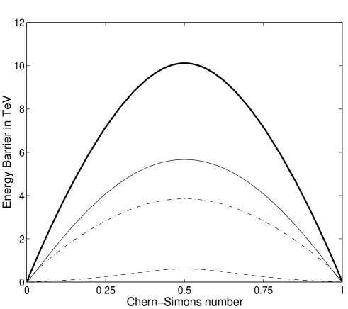
Figure 1: The sphaleron barrier for $m_{1}$=100 GeV, $m_{2}$=300 GeV, $m_{3}$=500 GeV, $\psi$=$\frac{\pi}{4}$, $\theta$=$\frac{\pi}{6}$, $\phi$=-$\frac{\pi}{4}$ and $\lambda_{3}$=0. The solid, dot-dashed and dashed lines are the contributions to the energy from the gauge field, the mixed or covariant derivative, and potential terms respectively.

The result, for one particular choice of masses and mixing angles, is shown in Fig. 1. The barrier showed no unusual features for having an extra doublet, and CP violation. In particular, it is symmetric around Chern-Simons number $\frac{1}{2}$. That this should be so is not obvious a priori, because $n_{CS}$ is odd under CP, and moreover changes by integer multiples under gauge transformations. Hence, a combination of a CP transformation and a large gauge transformation changes $n_{\mathrm{CS}}$ to $1-n_{\mathrm{CS}}$. It is therefore interesting that the barrier should be symmetric under this interchange when the underlying theory is not. It is also interesting to note the small contribution of the potential energy.

6 Energy as a function of CP violating angle

We were unable to find sensible values of $m_{1}$, $m_{2}$, $m_{3}$, $m_{H^{\pm}}$, $\phi$ and $\psi$, that satisfied Eqs. 39–42 for the entire range $0\leq\theta\leq\pi$. In turned out that the largest ranges of $\theta$ favoured degenerate $m_{1}$ and $m_{2}$, large $m_{3}$, and small $m_{H^{\pm}}$. We plotted height of the energy barrier as a function of $\theta$ for the allowed range. In Fig. 2 we display the energy as a function of the CP violating angle $\theta$, for $m_{1}$=100 GeV, $m_{2}$=110 GeV, $m_{3}$=500 GeV, $\psi=\frac{\pi}{8}$, $\phi=\frac{\pi}{8}$ and $\lambda_{3}$=0, values which are consistent with current bounds on Higgs masses [11].

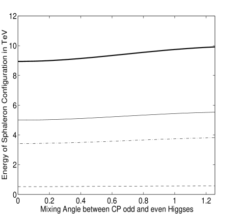
Figure 2: The sphaleron energy as a function of the CP violating Higgs mixing angle $\theta$, for Higgs masses $m_{1}$=100 GeV, $m_{2}$=110 GeV, $m_{3}$=500 GeV, and CP-conserving mixing angles $\psi=\frac{\pi}{8}$, $\phi=\frac{\pi}{8}$. The only coupling undetermined by the masses and the mixing angles is $\lambda_{3}$, which was set to zero. The solid, dot-dashed and dashed lines are the contributions to the energy from the gauge field, the mixed or covariant derivative, and potential terms respectively.

We note that the energy changes from 9 to 10 TeV over the range of $\theta$ we could obtain, or by roughly 10%. This is not insignificant, in view of the tightness of the upper bound on the lightest Higgs mass, which comes from the requirement that the sphaleron rate be sufficiently low in the symmetry-broken phase at the bubble nucleation temperature $T_{b}$. Increasing the sphaleron energy by this amount would mean that the ratio $\upsilon(T_{b})/T_{b}$ can be smaller, and hence that the transition can be more weakly first order. This means that the lightest Higgs is allowed to be more massive (see, e.g., [1] for a more detailed explanation).

Clearly, a more precise determination of the bounds must take into account finite temperature corrections, and use the true SU(2)$\times$U(1) theory. At the same time one should compute the ratio $\upsilon(T_{b})/T_{b}$ with the correct Higgs parameters. It is interesting to note that existing lattice calculations [7] assume that the Higgses in two-doublet models are not degenerate in mass, in order that all but the lightest can be integrated out. We find that in order to get large range of CP-violating angles, one must have almost degenerate light Higges. It may well be worth recalculating the strength of the transition as a function of the (zero-temperature) Higgs masses in the almost degenerate case.

7 Conclusions

In this paper we have made a start on investigating the effect of CP violation in the Higgs potential on the sphaleron energy, by looking at the sphaleron in the pure SU(2) two Higgs theory. We found firstly that the sphaleron energy changed by about 10% as we scanned though a range of our CP-violating parameter, which we defined to be the mixing of the CP-odd with the CP-even Higgs states. This indicates that it is worth going on to calculate the sphaleron energy with finite temperature corrections taken into account, and in the full SU(2)$\times$U(1) two Higgs theory. In this way the bounds deriving from the requirement that the baryon asymmetry not be destroyed in the symmetry-broken phase can be more precisely worked out. We also used a new method, that of gradient flow, to follow the fields as the sphaleron decays to the vacuum, and to exhibit the energy as a function of Chern-Simons number. The shape of the barrier shows no qualitative difference from that in CP-conserving theories: in particular, it is symmetric around Chern-Simons number $\frac{1}{2}$. In a CP-violating theory, this feature is not a priori obvious, and perhaps points to a deeper symmetry in the equations.

Finally, in order to relate our sphaleron energies to physical quantities, we adopted a novel strategy of computing as many as possible of the parameters of the Higgs potential from the masses and mixing angles of the Higgses. With four masses, three mixing angles, and the Higgs vacuum expectation value we needed to choose only two of the parameters without physical input. We found as a by-product that a large range of the CP-violating parameter could only be obtained if two of the Higgs were nearly degenerate in mass, and one much more massive. This again has important implications for the lattice calculations of the strength of the electroweak phase transition, which hitherto have assumed that the Higgses are well separated in mass.

8 Acknowledgements

We are indebted to Paul Saffin for his programming help. JG is supported by PPARC studentship 96314471 and MH by PPARC grant GR/L56305. Computational resources were made available by HEFCE and PPARC throught the JREI scheme.

References

• [1] V.A Rubakov and M.E. Shaposhnikov, Phys. Usp. 39, 461 (1996), hep-ph/9603208
• [2] M. Trodden, hep-ph/9803479
• [3] A.D. Sakharov, JETP Lett. 6 24 (1967).
• [4] G. ’t Hooft, Phys. Rev. Lett. 37 8 (1976).
• [5] F.R. Klinkhammer and N.S. Manton, Phys. Rev. D 30 2212 (1984).
• [6] V.A. Kuzmin, V.A. Rubakov, and M.E. Shaposhnikov, Phys. Lett. B 155 36 (1985).
• [7] K. Kajantie, M. Laine, K.Rummukainen, M. Shaposhnikov, and M. Tsypin, hep-ph/9809435
• [8] B. Kastening, R.D. Peccei, and X. Zhang, Phys. Lett. B 266 413 (1991).
• [9] C. Bachas, P. Tinyakov, and T.N. Tomaras, Phys. Lett. B 385 237 (1996), hep-ph/9606348
• [10] B. Kleihaus, hep-ph/9808295
• [11] C.A. Caso et al., European Physical Journal C3 1 (1998).
• [12] N. Manton, in “Formation and Interactions of Topological Defects”, NATO ASI Series, eds. R. Brandenberger and Davis, (Plenum, New York, 1995).
• [13] T. Akiba, H. Kikuchi, and T. Yanagida, Phys. Rev. D 38 1937 (1988).
• [14] G. Nolte and J. Kunz, Phys. Rev. D 51 3061 (1995), hep-ph/9409445
• [15] J.F. Gunion, H.E. Haber, G. Kane, and S. Dawson, “The Higgs Hunter’s Guide” (Addison-Wesley, Redwood City, 1990).
• [16] B. Ratra and L.G. Yaffe, Phys. Lett. B 205 57 (1988)
• [17] W. Press, S. Teukolsky, W. Veterling, and B. Flannery, “Numerical Recipies in C” (Cambridge Univ. Press, Cambridge, 1992).