NON-EQUILIBRIUM BOSE-EINSTEIN CONDENSATES, DYNAMICAL SCALING AND SYMMETRIC EVOLUTION IN THE LARGE N $\Phi^{4}$ THEORY

Abstract

We analyze the non-equilibrium dynamics of the $O(N)\;\Phi^{4}$ model in the large N limit with broken symmetry tree level potential and for states of large energy density. The dynamics is dramatically different when the energy density is above the top of the tree level potential $V_{0}$ than when it is below it. When the energy density is below $V_{0}$, we find that non-perturbative particle production through spinodal instabilities provides a dynamical mechanism for the Maxwell construction. The asymptotic values of the order parameter only depend on the initial energy density and all values between the minima of the tree level potential are available, the asymptotic dynamical ‘effective potential’ is flat between the minima. When the energy density is larger than $V_{0}$, the evolution samples ergodically the broken symmetry states, as a consequence of non-perturbative particle production via parametric amplification. Furthermore, we examine the quantum dynamics of phase ordering into the broken symmetry phase and find novel scaling behavior of the correlation function. There is a crossover in the dynamical correlation length at a time scale $t_{s}\approx\ln(1/\lambda)$. For $t<t_{s}$ the dynamical correlation length $\xi(t)\propto\sqrt{t}$ and the evolution is dominated by linear instabilities and spinodal decomposition, whereas for $t>t_{s}$ the evolution is non-linear and dominated by the onset of non-equilibrium Bose-Einstein condensation of long-wavelength Goldstone bosons. In this regime a true scaling solution emerges with a non-perturbative anomalous scaling length dimension $z=1/2$ and a dynamical correlation length $\xi(t)\propto(t-t_{s})$. The equal time correlation function in this scaling regime vanishes for $r>2(t-t_{s})$ by causality. For $t>t_{s}$ phase ordering proceeds by the formation of domains that grow at the speed of light, with non-perturbative condensates of Goldstone bosons and the equal time correlation function falls of as $1/r$. A semiclassical but stochastic description emerges for time scales $t>t_{s}$. Our results are compared to phase ordering in classical stochastic descriptions in condensed matter and cosmology.

I Introduction

Recent studies of non-equilibrium evolution of high energy density states have revealed novel and unexpected phenomena ranging from strong dissipative processes via particle production[1, 2] to novel aspects of symmetry breaking[3, 4]. These non-equilibrium effects are crucial to understanding the end of inflation and the reheating problem[2, 5, 6]. They are also conjectured to be relevant for baryogenesis, the partial restoration of symmetries during phase transitions[7, 8], for the formation of defects during non-equilibrium phase transitions[8, 9] and reheating dynamics in gauge and fermionic theories[10]. More recently a novel form of anomalous relaxation with non-universal critical exponents[11] has been found in scalar field theories due to non-equilibrium quantum effects.

One of the important aspects of these phenomena are their non-perturbative character. There are few consistent approaches that can be used for their description. While a classical approach has been advocated to address these issues[5, 7, 8, 9] we have emphasized the application of the large $N$ limit that captures both the quantum aspects as well as the emergence of classicality[1, 2, 3, 4, 6, 11]. The large $N$ limit in scalar field theories has a consistent implementation within the non-equilibrium quantum field theory formulation[1, 2, 12] and the renormalization aspects had been studied in detail[13, 14]. Furthermore it provides a consistent, renormalizable framework to study non-perturbative phenomena that can be systematically improved[1, 2, 12].

In this article we focus on further new non-equilibrium aspects. First, we discuss how non-perturbative particle production due to spinodal instabilities gives rise to a dynamical version of the Maxwell construction of statistical mechanics. It is a well known result that the static effective potential becomes complex in the region of the phase diagram in which coexistence of phases can occur. The imaginary part has been deemed to arise from a failure of the loop expansion, but a more careful treatment reveals that this imaginary part is actually related to the decay rate of a quantum mechanically unstable state[15, 16]. More precisely, the static effective potential approach is just not appropriate to study the dynamic of phase transitions. At the level of formal statistical mechanics, the mixed phase is described via a Maxwell construction that leads to an effective potential (free energy) that is flat in the coexistence region. The Maxwell constructed effective potential has been confirmed by a careful analysis using the ‘exact’ renormalization group[17, 18, 19] of the equilibrium coarse grained free energy.

Here we study the dynamical aspects of the Maxwell construction in the large $N$ limit of a scalar field theory. We begin by reviewing the relevant features of the static effective potential in the large $N$ limit[20, 21, 22] to highlight the fact that the imaginary part of the effective potential is not an artifact of the loop expansion but a more fundamental shortcoming of a static and equilibrium description of the coexistence region in terms of an homogeneous order parameter. We then study in detail how non-equilibrium dynamics, and in particular, particle production due to spinodal instabilities, leads to a flat dynamic potential in the region of coexistence. We find that all expectation values of the scalar field between the minima of the tree level potential are available asymptotically and that the asymptotic value is reached with a vanishing effective mass for the expectation value. This is the dynamical equivalent of a ‘flat dynamical potential’ and the availability of all possible asymptotic expectation values between the minima is the dynamical equivalent of the lever rule for coexistence of phases in the Maxwell construction. For a given initial expectation value, such that the total energy density, $\varepsilon$, is smaller than the maximum of the tree level potential $V(0)$, [here $V(\Phi)$ is the potential for the $O(N)$ field $\Phi$], we find that the asymptotic expectation value depends on the initial conditions only through the total energy as follows

$$<\Phi({\vec{x}},\infty)>=\sqrt{2\over\lambda}|m|\left[1-{\varepsilon\over V(0)}\right]^{x}$$

where $\lambda$ and $m$ are the renormalized quartic self-coupling and mass respectively and $x$ a new dynamical anomalous exponent which is universal in the weak coupling limit and given by $x=0.25$.

In summary, the dynamical effective potential is always real and is flat for $\varepsilon<V(0)$. Two physically different situations appear here:

a) when the energy density $\varepsilon$ is smaller than the maximum of the tree level potential, $\varepsilon<V(0)$ (in terms of renormalized mass and coupling), the non-equilibrium dynamical evolution leads to broken symmetry states and the Maxwell construction via non-perturbative particle production as a consequence of the spinodal instabilities.

b) when $\varepsilon>V(0)$, in which case the energy density is larger than the maximum of the tree level potential, we find that the evolution is symmetric in that the time evolution of the expectation value of the scalar field samples the minima of the tree level potential symmetrically and ergodically with vanishing average over time scales much longer than the period. What we find is that this evolution is a consequence of the growth of the root mean square fluctuations due to parametric amplification which eventually induces a positive mass squared for the field. We show numerically that the expectation value relaxes to zero asymptotically transferring all of the energy to quantum fluctuations via parametric amplification in accord with the results in[6, 11].

Our final topic concerns the quantum non-equilibrium dynamics of phase ordering in the $O(N)$ model. This is an important topic and is the basis of the Kibble mechanism for defect formation as the early universe cools through phase transitions[23, 24, 25]. Recently, there have been some attempts at constructing a non-equilibrium, real-time, description of the dynamics of this process[26]. The early stages of the dynamics of phase ordering in quantum field theory models begin with the growth of spinodally unstable long-wavelength field modes and a dynamical correlation length emerges[27]. The dynamics of non-equilibrium fluctuations during the early spinodally unstable stage has been studied and clarified recently providing a deeper understanding of the quantum fluctuations that trigger the process of phase ordering[28, 29]. We go beyond the early and intermediate time regime which is dominated by the linear instabilities, into the highly non-linear regime which is dominated by non-linear resonances[11] and that begins at the spinodal time $t_{s}\sim m^{-1}\ln(1/\lambda)$. This time scale determines the emergence of a semiclassical but stochastic description which we discuss and clarify. After $t_{s}$, semiclassical, large amplitude ($\propto 1/\sqrt{\lambda}$) field configurations are represented in the quantum density matrix with unsupressed probability.

We find that for $t>t_{s}$ a true scaling solution emerges for which the field acquires a non-perturbative anomalous scaling (length) dimension $z=1/2$, a dynamical correlation length $\xi(t)\approx(t-t_{s})$ emerges. In and the equal-time correlation function vanishes by causality at distances $r>2(t-t_{s})$. In the non-linear regime we find the onset of a novel form of Bose Einstein condensation in which the zero momentum mode of the quantum fluctuations grows asymptotically linearly in time becoming macroscopically populated at long times. This condensation mechanism results in the equal time correlation function decreasing as $1/r$ for $r<2(t-t_{s})$ as a consequence of massless excitations. We find a crossover in the time dependence of the dynamical correlation length at the spinodal time $t_{s}$:

$$\xi(t)\approx\sqrt{t}\quad\mbox{for}\quad t<t_{s}\quad;\quad\xi(t)\approx t-t_{s}\;\quad\mbox{for}\quad t>t_{s}\;.$$

The process of phase ordering in this regime is described by the formation of domains that grow at the speed of light, inside of which there is a non-perturbative condensate of Goldstone bosons.

In section II we review the construction of the effective potential in the large $N$ limit and highlight several important features that are relevant for the dynamics namely

• the regime of validity of the scalar field theory as an effective theory below the energy scale of the Landau pole $\approx m\;e^{16\pi^{2}/\lambda}\;$, and the consistency of studying this theory for energy densities $\propto m^{4}/\lambda$,

• the complex result for the effective potential in the coexistence region and the failure of such effective potential to describe dynamical aspects. In the large $N$ limit, this effective potential is exact and this complex value cannot be blamed on a failure of the loop expansion but is a consequence of more fundamental shortcomings of an effective potential description.

In section III we set up our study of the non-equilibrium dynamics in terms of the quantum density matrix in the large $N$ limit and its probabilistic interpretation. This formulation is the most enlightening to use use in order to discuss the emergence of classicality in terms of probability distributions. It also provides a natural framework in which to interpret the formation of semiclassical, large amplitude, field configurations that are represented in the quantum ensemble with unsuppressed probabilities.

Section IV is devoted to a detailed study of the dynamics in a broken symmetry potential. Here we distinguish between symmetric and non-symmetric evolution and provide a simple criterion for ergodic symmetric evolution in a broken symmetry potential. We contrast the energy with the effective potential and show that particle production provides a dynamical mechanism for the Maxwell construction. Section VI deals with the non-equilibrium process of phase ordering both in the linear and in the non-linear regime. We then compare our results to those of phase ordering kinetics in condensed matter physics[30, 31] and the scaling solution found in radiation and matter dominated Friedmann-Robertson-Walker cosmologies for the non-linear sigma model[32, 33]. We summarize our results and conclusions in section VII.

II The Effective Potential in the large $N$ limit

One of the main conclusions of our work is that the understanding of field theories to be found in the effective potential can be woefully lacking under certain circumstances. In order to better compare and contrast our dynamical results with what would have been expected from an effective potential analysis, and since there are some subtleties involved in the discussion of the large $N$ limit effective potential[20, 21, 22], we recapitulate this discussion below.

There are two facets of the $O(N)$ effective potential that we want to make contact with:

• Scalar field theories can only be taken as effective field theories with a restricted regime of validity. The $O(N)$ model is known to have a Landau ghost at an energy scale $\approx m\;e^{16\pi^{2}/\lambda}$, with $m\;;\;\lambda$ the renormalized mass and coupling respectively, and can only be used reliably below this energy scale. A fuller analysis of the $O(N)$ effective potential in the large $N$ limit determines the range of energy densities for which the theory can make sensible predictions.

• The effective potential is complex in the spinodal region. This is what gives rise to the standard Maxwell construction. We want to understand the dynamics associated with this construction.

We consider the $O(N)$ vector model with Lagrangian density given by,

$${\cal{L}} = \frac{1}{2}\,\dot{\vec{\Phi}}(\vec{x},t)^{2}-\frac{1}{2}\,(\vec{\nabla}\vec{\Phi}(\vec{x},t))^{2}-V(\vec{\Phi}(\vec{x},t))$$ (1)

$$V(\vec{\Phi}) = \frac{1}{2}m^{2}_{0}\,\vec{\Phi}^{2}+\frac{\lambda_{0}}{8N}\,(\vec{\Phi}^{2})^{2}+{N\,m^{4}_{0}\over 2\,\lambda_{0}}$$ (2)

To analyze the large $N$ limit it proves convenient to introduce a Lagrange multiplier field $\alpha(x)$[12] and write the above Lagrangian density in the form

$${\cal{L}}=\frac{1}{2}\,\dot{\vec{\Phi}}(\vec{x},t)^{2}-\frac{1}{2}\,[\vec{\nabla}\vec{\Phi}(\vec{x},t)]^{2}+\frac{N\;}{2\lambda_{0}}\;(\alpha(\vec{x},t)-2\,m^{2}_{0})\;\alpha(\vec{x},t)-\frac{1}{2}\,\vec{\Phi}(\vec{x},t)^{2}\;\alpha(\vec{x},t)$$

The effective potential ($V_{eff}$) can be obtained in the $N=\infty$ limit in the following manner[20, 21, 22]: introducing the expectation value of the scalar field as $\phi(\vec{x},t)^{2}\equiv\frac{1}{N}<\Phi(\vec{x},t)^{2}>$, the quadratic functional integral over the field $\Phi(\vec{x},t)$ can be performed exactly leading to an effective functional of the Lagrange multiplier $\alpha(\vec{x},t)$ and the expectation value $\phi(\vec{x},t)^{2}$. The leading order in the large $N$ limit is obtained via the saddle point approximation in the functional variable $\alpha(\vec{x},t)$ and expansion around the saddle point generates a series in powers of $1/N$. Translational invariance dictates that the relevant saddle point solution must be a space-time constant. In the large $N$ limit only coupling and mass renormalization are needed:

$$\frac{m^{2}_{0}}{\lambda_{0}} = \frac{m^{2}}{\lambda}-\frac{\Lambda^{2}}{16\pi^{2}}$$ (3)

$$\frac{1}{\lambda_{0}} = \frac{1}{\lambda}-\frac{1}{32\pi^{2}}\ln\left[\left(\frac{2\Lambda}{|m|}\right)^{2}\frac{1}{e}\right],$$ (4)

where $\Lambda$ is an ultraviolet cutoff and the finite part in the renormalization of the coupling (4) has been conveniently chosen to simplify the expressions below. As a function of $\alpha(x)=M^{2}$, and $\phi^{2}$, the effective potential at leading order in the large $N$ limit is:[20, 21, 22]

$$V_{eff}(\phi^{2},M^{2})=\frac{M^{2}}{2}\left[\phi^{2}-{{M^{2}-2m^{2}}\over{\lambda}}-{{M^{2}}\over{32\pi^{2}}}\log\left({{\sqrt{e}\,|m|^{2}}\over{M^{2}}}\right)\right],$$ (5)

where $m$ and $\lambda$ are the renormalized mass and coupling, and we have chosen $|m|^{2}$ to be the renormalization scale. Extremizing with respect to the saddle point solution for the Lagrange multiplier, $M^{2}$ we are led to the gap equation[20, 21, 22]:

$$\phi^{2}(M^{2})={{2(M^{2}-m^{2})}\over{\lambda}}+{{M^{2}}\over{16\pi^{2}}}\log\left({{|m|^{2}}\over{M^{2}}}\right)$$ (6)

Shifting the Lagrange multiplier field $\alpha(x)$ by the saddle point value $M^{2}$ we identify $M^{2}$ as the effective squared mass of the fluctuations of the $\vec{\Phi}$ field.

We see from eq.(6) that $\phi^{2}(M^{2})$ increases with $M^{2}$ for $M^{2}<|m|^{2}\;e^{32\pi^{2}/\lambda-1}$.

The effective potential at the solution of the gap equation becomes

$$V_{eff}(\phi^{2}(M^{2}),M^{2})=\frac{M^{4}}{16}\left[\frac{8}{\lambda}+{1\over{4\pi^{2}}}\log\left({{|m|^{2}}\over{\sqrt{e}\,M^{2}}}\right)\right]$$ (7)

It proves convenient to introduce the following dimensionless variables:

$$w \equiv e^{-32\pi^{2}/\lambda}\;{M^{2}\over|m|^{2}}$$ (8)

$$v(w) \equiv {32\pi^{2}\over m^{4}}\;e^{-64\pi^{2}/\lambda}\;V_{eff}(\phi^{2}(M^{2}),M^{2})$$ (9)

$$\varphi^{2} \equiv {16\pi^{2}\over|m|^{2}}\;e^{-\frac{32\pi^{2}}{\lambda}}\;\phi^{2}$$ (10)

in terms of which

$$v(w)=-\frac{1}{2}w^{2}\left(\frac{1}{2}+\log w\right)\;.$$ (11)

In fig. 1 we plot the dimensionless function $v(w)$ vs. $w$. Furthermore at the solution of the gap equation we find the relation

$$\varphi^{2}(w)=-{32\pi^{2}\over\lambda}\mbox{sign}(m^{2})\;e^{-32\pi^{2}/\lambda}-w\log w\;.$$ (12)

In the regime of interest where $\lambda/(32\pi^{2})$ is small, the dimensionless variables $v,w$ and $\varphi$ contain the very small factor $\,e^{-32\pi^{2}/\lambda}\,$ times factors that are typically of order one. Hence, the physically interesting domain of values for $v,w$ and $\varphi$ is near the origin. Only for energies near the Landau ghost, $v,w$ and $\varphi$ become of order one.

Hence, in the infinite $N$ limit, the (‘pion’) field $\Phi_{a}\;(1\leq a\leq N)$ is a free field with mass squared equal to $M^{2}$.

On the other hand, the composite field ${\vec{\Phi}}^{2}(x)$ has as inverse propagator in euclidean space time given by

$$\Delta(k)=\Delta(0)+{1\over{(4\pi)^{2}}}\;\int_{0}^{1}dx\;\log\left[1+x(1-x){{k^{2}}\over{M^{2}}}\right]$$ (13)

where

$$\Delta(0)=-\frac{2}{\lambda}-{1\over{16\pi^{2}}}\log\left({{|m|^{2}}\over{e\;M^{2}}}\right)$$ (14)

The relevance and properties of this propagator will be investigated below for the cases of unbroken $m^{2}>0$ and broken $m^{2}<0$ symmetry.

It is clear from the gap equation (6) and fig. (1) , that $\phi^{2}$ as a function of $M^{2}$ has a maximum at

$$M^{2}=M^{2}_{0}\equiv|m|^{2}\,\exp\left({{32\pi^{2}}\over\lambda}-1\right)$$ (15)

for real $M^{2}$. Notice that such mass scale is of the order of the Landau ghost. That means that it is outside the expected domain of validity of the $\left({\vec{\Phi}}^{2}\right)^{2}$, which can be used as an effective theory for energies well below the Landau ghost.

At the maximum of $\phi^{2}=\phi^{2}(M^{2})$, we have

$$\phi^{2}_{0}\equiv\phi^{2}(M^{2}_{0})={{M^{2}_{0}}\over{16\pi^{2}}}-{{2\,m^{2}}\over{\lambda}}\;.$$ (16)

This value is also of the order of the Landau ghost for our choice of $m^{2}$.

Therefore, for scales much lower than the Landau ghost, the $(\vec{\Phi}^{2})^{2}$ theory is a sensible low energy effective description. In particular in our studies of the dynamics the scale of the expectaction value is typically of order $\phi^{2}\approx|m|^{2}/\lambda<<\phi^{2}_{0}$ which is well within the regime of validity of the effective theory for weak coupling.

As observed in [21, 22], the inverse function $M^{2}=M^{2}(\phi^{2})$ has two branches as a function of $\phi^{2}$. However, the second branch, $M^{2}>M^{2}_{0}$, (branch II in [21]) corresponds to pion masses beyond the Landau ghost. A consistent low energy effective theory emerges for energies well below $M^{2}_{0}$ [See ref[22], sec. IIIA]. This low energy condition requires that this scalar field theory be studied with a finite but large ultraviolet cutoff $|m|<<\Lambda<<|m|\;e^{16\pi^{2}/\lambda}$ and a positive coupling $\lambda$.

A Analysis of the gap equation and the effective potential for $m^{2}>0$

Equation (6) and fig. 1 reveal that for $m^{2}>0$, the gap equation has a real and positive solution for $0\leq\phi^{2}\leq\phi^{2}_{0},\;M^{2}_{1}\leq M^{2}\leq M^{2}_{0}$ where $M^{2}_{1}$ corresponds to $\phi^{2}=0$. The field $\phi$ becomes complex and hence unphysical for $M^{2}\leq M^{2}_{1}$.

In fig. 2, the point

$$w_{1}\equiv e^{-32\pi^{2}/\lambda}\;\frac{M^{2}_{1}}{m^{2}}\;.$$

corresponds to the intersection of the lower curve (unbroken symmetry) with the $\varphi=0$ axis. $w_{1}$ is thus the positive solution of the trascendental equation

$$w_{1}\log w_{1}=-\frac{32\pi^{2}}{\lambda}\;e^{-\frac{32\pi^{2}}{\lambda}}\;.$$

[cfr. eq.(12)] which defines the value of $M^{2}_{1}$.

Clearly, the effective potential is minimal for $\phi^{2}=0,\;M^{2}=M^{2}_{1}$. This is the $O(N)$ symmetric ground state with pions of mass $M^{2}_{1}>0$ [22].

The study of the field theory dynamics in this unbroken symmetry case for initial excited states[11] shows that the (time dependent) effective mass tends to a nonzero value for late times. The pions are thus massive and the zero mode slowly dissipates its energy (there is a non-zero threshold for particle production) and attains the ground state ($\phi=0$) very slowly, with an oscillatory behavior modulated in amplitude by a power law with anomalous relaxation exponent for asymptotically large time[11].

We see that the static analysis through the effective potential agrees with the long time dynamics in the sense that the expectation value of the scalar field relaxes to the minimum of the effective potential, i.e. $\phi=0$ with oscillations that reflect a non-zero mass. In addition, the effective pion mass obtained asymptotically in the dynamical situation depends on the initial energy density (which is conserved)[11]. This dependence of course cannot be captured by a static analysis which only applies to the ground state.

The ${\vec{\Phi}}^{2}$ propagator given by eqs.(13-14) has a tachyonic pole at $\Delta(m_{T})=0$, if $\Delta(0)<0$. This occurs for $M^{2}<m^{2}\;\exp\left({{32\pi^{2}}\over\lambda}-2\right)$. That is, a tachyon is present unless the pion mass is of the order (or larger) than the Landau ghost. In particular, tachyons are absent if one chooses the second branch of the function $M^{2}=M^{2}(\phi^{2})$ [21]. As stated before, this scalar theory should only be interpreted to be valid as a low energy effective theory with $\log\frac{M^{2}}{m^{2}}=O(1)$. The tachyon is then present but at a very large mass provided $\lambda$ is small. We find from eqs.(13-14),

$$\Delta(k)\buildrel k\to\infty\over{=}-\frac{2}{\lambda}+{1\over{(8\pi)^{2}}}\log\left({k\over{m\,\sqrt{e}}}\right)+O({1\over{k^{2}}})\;.$$

Thus the tachyon mass

$$m_{T}=m\;\exp\left({{16\pi^{2}}\over\lambda}+\frac{1}{2}\right)\;.$$

is beyond the range of validity of the effective $\left({\vec{\Phi}}^{2}\right)^{2}$ theory.

In particular in our studies of the dynamics the typical expectation values are of order $\phi^{2}\approx m^{2}/\lambda$ and for these energy scales ${\cal O}(m/\sqrt{\lambda})$ the ultra-heavy tachyonic states are never excited and they decouple from the low energy theory. We can thus safely ignore the existence of the tachyon.

B Analysis of the gap equation and the effective potential for $m^{2}<0$

In this case, it is clear from eq.(6) and fig. 2 that $\phi^{2}\geq{{2\,|m|^{2}}\over{\lambda}}$ for $M^{2}$ real in the interval $0\leq M^{2}\leq M^{2}_{0}$ with $M^{2}_{0}$ given by eq.(15). Equation (7) and fig. 2 show that the minimum of the effective potential corresponds to $M^{2}=0,\;\phi^{2}={{2\,|m|^{2}}\over{\lambda}}$. That is,

$$\varphi^{2}(w)\geq\varphi^{2}(0)=\frac{32\pi^{2}}{\lambda}\;e^{-\frac{32\pi^{2}}{\lambda}}$$

for real $0\leq w\leq 1/e$. The minimum of $V_{eff}$ is at the point $w=0$ in the upper curve (broken symmetry) in fig. 2.

This yields a broken $O(N)$-symmetry ground state. As expected, we have $N-1$ massless pions which are the Goldstone bosons of the $O(N)\to O(N-1)$ breaking [22] as can be seen from eq.(7) and fig. 2 which show that $M^{2}=0$ is the minimum of the effective potential for $M^{2}\geq 0$ and below the Landau ghost. However, this value corresponds to a non-negative $\phi^{2}$ only for $m^{2}<0$. The fact that the minimum $M^{2}=0$ of the effective potential happens in the real configuration space (for $m^{2}<0$) is in agreement with the asymptotic late time behavior found in refs.[1, 2, 6, 11]. There it was found that the dynamical (time dependent) effective mass of the pion fields tends asymptotically to zero for $m^{2}<0$ (and initial energy below the false vacuum but above the ground state). The presence of massless particles allows the zero mode energy to dissipate efficently into them and the zero mode rapidly reaches the ground state. This happens very slowly in the $m^{2}>0$ case (unbroken symmetry). In this case the pions are massive and energy dissipation occurs via non-linear resonances[11].

Now we come to one of the important features of the effective potential in the broken symmetry phase: it follows from eqs.(11), (12) and (16) that there is no real solution $M^{2}$ (or $w$) for $\phi^{2}>\phi^{2}_{0}$. Therefore, $M^{2}$ and $w$ as well as the effective potential become complex despite of the fact that the field $\phi^{2}$ is real.

Whereas in a loop expansion this imaginary part is typically ignored with the hope that higher order corrections (loops) could remedy this situation, in the large $N$ limit this argument does not hold. The physics associated with the imaginary part of the effective potential has been clarified in references[15, 16].

In the region in which the effective potential computed from eq.(7) or eq.(11) turns to be complex, referred to as the spinodal region, the system is in a mixed state in which several phases coexist. The true equilibrium description of the system in the spinodal region is in terms of a Maxwell constructed effective potential, which is flat in the coexistence region $0\leq\phi^{2}\leq{{2\,m^{2}}\over{\lambda}}$[17]. Although such construction is rather arbitrary at the level of phenomenological statistical mechanics (the lever rule), a consistent renormalization group analysis has revealed that the infrared limit of a carefully coarse grained effective action yields the Maxwell constructed effective potential[17]. We also note that in this case of continuous symmetry the spinodal region extends all the way from the maximum to the minimum of the potential without a region of metastability. This must be contrasted with the case of discrete symmetry, wherein the spinodal ends in the limit of metastability before the minimum of the potential. The fact that the spinodal region reaches from the maximum to the minimum of the potential is a consequence of the presence of Goldstone bosons.

At this point we summarize the relevant features of the effective potential in the large $N$ limit to compare to the results obtained from the dynamical evolution[1, 2].

• In the unbroken symmetry case with positive renormalized mass squared ($m^{2}>0$) the static effective potential has a unique minimum for a nonzero value of the squared mass $M^{2}$ of the excitations and vanishing expectation value of the field $\phi$. The dynamics agrees with a vanishing expectation value of the field reached asymptotically at late times with power laws[11]. In addition, the asymptotic effective mass obtained from the dynamical evolution depends on the initial expectation value of the field[11].

• The analysis of ref.[22] shows that the $O(N)$ symmetry is broken in the effective theory for $m^{2}<0$ where again, by effective theory we imply describing energies well below the Landau ghost scale $M^{2}_{0}$ [see eq.(15)].

  When the renormalized mass $m^{2}<0$, the minimum of the static effective potential is found at $M^{2}=0$ and for a nonzero value of the field $\phi$. The $O(N)$ symmetry is then spontaneously broken and the massless scalars are the corresponding Goldstone bosons. The static effective potential computed from eq.(7) or eq.(11) is complex in the interval $0<\phi^{2}<2|m|^{2}/\lambda$; this is the spinodal region that signals phase coexistence. The spinodal region reaches from the maximum to the minimum of the potential unlike in the discrete symmetry case.

  The physics inside the spinodal region cannot be captured via a static description. An equilibrium description of this region can be given in terms of the Maxwell construction which leads to a flat effective potential for $0<\phi^{2}<2m^{2}/\lambda$. Such a description emerges in quantum field theory with a consistent treatment using the exact renormalization group[17, 18, 19]. In the next sections we will study the dynamical Maxwell construction that leads to a flat dynamical effective potential in the spinodal region via the non-equilibrium dynamics.

  In section IV we study the dynamics of evolution in a broken symmetry case but when the initial value of $\phi$ is above the maximum of the tree level potential. In this case the dynamics is similar to that of the unbroken symmetry case. The effective potential is simply unable to describe correctly this physical situation.

• Furthermore, the effective potential clearly illuminates the regime of validity of the scalar theory as an effective, cutoff low energy theory below the Landau ghost. Obviously, the physics is radically different when one considers pions and/or field expectations values at the energy scale of the Landau ghost. Our study of the dynamics in both the broken and unbroken symmetry phases will be restricted to energy scales $\approx|m|/\sqrt{\lambda}$ and energy densities $\approx m^{4}/\lambda$ i.e. well below the Landau ghost scale for weak coupling. Therefore this scalar theory is a reliable cutoff low energy model to study the non-perturbative dynamics for energy scales below the Landau ghost.

III Non-Equilibrium Dynamics in the large $N$ limit: The Density Matrix

The field theory tool to study non-equilibrim dynamics is the quantum density matrix $\hat{\rho}(t)$ which obeys the functional Liouville equation

$$i\frac{\partial\hat{\rho}}{\partial t}=\left[H(t),\hat{\rho}\right]$$

where we admit a Hamiltonian that can depend explicitly on time as it would be the case in expanding cosmologies. A particularly illuminating representation for the field theoretical density matrix is the Schrödinger representation[14, 3], in which the field operator is diagonal. In such a representation

$$\rho[\Phi(\cdot),\tilde{\Phi}(\cdot);t]=\langle\Phi|\hat{\rho}(t)|\tilde{\Phi}\rangle$$

and the diagonal density matrix elements $\rho[\Phi(\cdot),{\Phi}(\cdot);t]={\cal{P}}(\Phi;t)$ give the functional probability density for finding a field configuration with profile $\Phi(\vec{x})$ at time t. Therefore, this representation allows to ask questions about the formation of semiclassical configurations in terms of probability functionals. This is the correct interpretation for the question of finding any arbitrary field configuration in the ensemble described by the non-equilibrium density matrix.

We will study the general case of a biased initial condition leading to symmetry breaking dynamics to illuminate various features of the non-equilibrium dynamics and the implementation of Goldstone’s theorem. Therefore we write

$$\vec{\Phi}(\vec{x},t) = \left(\sqrt{N}\phi(t)+\sigma(\vec{x},t),\vec{\Psi}(\vec{x},t)\right)$$ (17)

$$\langle\Phi^{a}(\vec{x},t)\rangle = \sqrt{N}\;\phi(t)\;\delta^{a,1}=Tr\left[\hat{\rho}(t)\Phi^{a}(\vec{x})\right]$$ (18)

and $\vec{\Psi}$ is an $O(N-1)$ vector.

The canonical momenta conjugate to $\sigma$ and $\Psi^{a}$ are given by

$$\Pi_{\sigma}(\vec{x},t)=\dot{\sigma}(\vec{x},t)\;\;;\;\;\Pi^{a}_{\Psi}(\vec{x},t)=\dot{\Psi}^{a}(\vec{x},t)$$

and the Hamiltonian becomes

$$H(t)=\int d^{3}x\left\{\frac{1}{2}{\Pi^{2}_{\sigma}}+\frac{1}{2}\vec{\Pi}^{2}_{\Psi}+\frac{1}{2}(\vec{\nabla}\Phi)^{2}+\frac{1}{2}(\vec{\nabla}\vec{\Psi})^{2}+V(\phi,\sigma,\vec{\Psi})\right\}+\frac{N}{2}\dot{\phi}^{2}(t)$$

In the Schrödinger representation (at an arbitrary fixed time $t_{0}$), the canonical momenta are represented as functional derivatives

$$\Pi_{\sigma}(\vec{x}) = -i\frac{\delta}{\delta\sigma(\vec{x})}$$ (19)

$$\Pi^{a}_{\Psi}(\vec{x}) = -i\frac{\delta}{\delta\Psi^{a}(\vec{x})}$$ (20)

and the Liouville equation for the density matrix becomes a functional differential equation[14]

$$i<\Psi,\sigma|\dot{\rho}(t)|\tilde{\sigma},\tilde{\Psi}>=\left(H[\Pi_{\sigma},\vec{\Pi}_{\Psi},\sigma,\vec{\Psi};t]-H[\tilde{\Pi}_{\sigma},\vec{\tilde{\Pi}}_{\Psi},\tilde{\sigma},\vec{\tilde{\Psi}};t]\right)<\Psi,\sigma|\rho(t)|\tilde{\sigma},\tilde{\Psi}>.$$ (21)

The large $N$ limit can be implemented by introducing an auxiliary field or alternatively using the following factorization

$$\sigma^{4} \rightarrow 6\langle\sigma^{2}\rangle\sigma^{2}+\mbox{ constant }$$ (22)

$$\sigma^{3} \rightarrow 3\langle\sigma^{2}\rangle\sigma$$ (23)

$$(\vec{\Psi}\cdot\vec{\Psi})^{2} \rightarrow 2\langle\vec{\Psi}^{2}\rangle\vec{\Psi}^{2}-\langle\vec{\Psi}^{2}\rangle^{2}$$ (24)

$$\vec{\Psi}^{2}\sigma^{2} \rightarrow \vec{\Psi}^{2}\langle\sigma^{2}\rangle+\langle\vec{\Psi}^{2}\rangle\sigma^{2}$$ (25)

$$\vec{\Psi}^{2}\sigma \rightarrow \langle\vec{\Psi}^{2}\rangle\sigma,$$ (26)

where the constant term in (22) is irrelevant as it will give a subleading correction in the large $N$ limit. In this approximation, the potential (2) becomes

$$V(\phi,\sigma,\vec{\Psi}) = V(\sqrt{N}\phi)+\sigma\;{\cal{V}}^{1}(t)+\frac{M^{2}_{\sigma}(t)}{2}\;\sigma^{2}+\frac{M^{2}(t)}{2}\;\vec{\Psi}^{2}$$ (27)

$$V(\sqrt{N}\phi) = {N\,\lambda\over 8}\left(\phi^{2}-{2\,m^{2}\over\lambda}\right)^{2}$$ (28)

$${\cal{V}}^{1}(t) = \sqrt{N}\phi(t)\left[m^{2}+\frac{\lambda}{2}\phi^{2}(t)+\frac{\lambda}{2N}\langle\vec{\Psi}^{2}\rangle(t)\right]$$ (29)

$${M}^{2}(t) = m^{2}+\frac{\lambda}{2}\phi^{2}(t)+\frac{\lambda}{2N}\langle\vec{\Psi}^{2}\rangle(t)$$ (30)

$${M}^{2}_{\sigma}(t) = m^{2}+\frac{3\lambda}{2}\phi^{2}(t)+\frac{\lambda}{2N}\langle\vec{\Psi}^{2}\rangle(t)$$ (31)

Since in this approximation the evolution Hamiltonian is quadratic (at the expense of a self-consistency condition), and the different $O(N)$ components evolve independently, the density matrix factorizes as[14]

$$\rho(t)=\rho_{\sigma}(t)\otimes\rho_{\Psi}(t)$$ (32)

Furthermore, the density matrices can be chosen to be Gaussian, and will remain Gaussian under time evolution.

Using spatial translational invariance, we can decompose the fields into their spatial Fourier modes and use these as a basis for the Schrödinger representation density matrix:

$$\sigma(\vec{x},t) = \int\frac{d^{3}k}{(2\pi)^{3/2}}\;\sigma_{\vec{k}}(t)\;\exp(-i\vec{k}\cdot\vec{x})$$ (33)

$$\vec{\Psi}(\vec{x},t) = \int\frac{d^{3}k}{(2\pi)^{3/2}}\;\vec{\Psi}_{\vec{k}}(t)\;\exp(-i\vec{k}\cdot\vec{x})\;.$$ (34)

The Gaussian density matrices acquire a simple form in terms of these Fourier modes[14]

$$\rho_{\sigma}[\sigma,\tilde{\sigma},t] = \prod_{\vec{k}}{\cal{N}}_{\sigma,k}(t)\;\exp\left\{-\frac{A_{\sigma,k}(t)}{2}\;\sigma_{k}(t)\sigma_{-k}(t)-\frac{A^{*}_{\sigma,k}(t)}{2}\;\tilde{\sigma}_{k}(t)\tilde{\sigma}_{-k}(t)\right.$$ (35)

$$- \left.B_{\sigma,k}(t)\sigma_{k}(t)\tilde{\sigma}_{-k}(t)+ip_{\sigma,_{k}}(t)\left[\sigma_{-k}(t)-\tilde{\sigma}_{-k}(t)\right]\right\}\;,$$ (36)

$$\rho_{\vec{\Psi}}[\vec{\Psi},\tilde{\vec{\Psi}},t] = \prod_{\vec{k}}{\cal{N}}_{\Psi,k}(t)\exp\left\{-\frac{A_{\Psi,k}(t)}{2}\;\vec{\Psi}_{k}\cdot\vec{\Psi}_{-k}-\frac{A^{*}_{\Psi,k}(t)}{2}\;\tilde{\vec{\Psi}}_{k}\cdot\vec{\tilde{\Psi}}_{-k}\right.$$ (37)

$$- \left.B_{\Psi,k}(t)\;\vec{\Psi}_{k}\cdot\tilde{\vec{\Psi}}_{-k}\right\}\;.$$ (38)

Only the component along the broken symmetry direction, $\sigma$ has an expectation value of the momentum, represented by $p_{\sigma,k}(t)$ in (36), whereas the transverse directions have vanishing expectation value of the momentum. The kernels $A_{\Psi};\;B_{\Psi}$ are scalars under $O(N-1)$. Although we will ultimately work at zero temperature, we have written the most general form of the density matrix, including a mixing term given by the kernels $B_{\sigma,\Psi,k}$ above to display the most general form of the density matrix. When the mixing kernels $B_{\sigma,\Psi,k}$ vanish, the density matrix collapses to a product of a wave functional and its complex conjugate, i.e. it describes a pure state. Also note that hermiticity of the density matrix requires that the mixing kernels $B_{\sigma,\Psi}$ be real.

Now the Liouville equation (21) can be solved for the time dependent kernels by comparing the different powers of $\sigma,\Psi$ on both sides of the equation (21). We obtain the following set of evolution equations for the kernels[14]:

$$i\,\frac{{\dot{\cal{N}}}_{\sigma,k}}{{\cal{N}}_{\sigma,k}} = \frac{1}{2}(A_{\sigma,k}-A^{*}_{\sigma,k})$$ (39)

$$i\dot{A}_{\sigma,k} = A^{2}_{\sigma,k}-B^{2}_{\sigma,k}-\omega^{2}_{\sigma,k}(t)$$ (40)

$$i\dot{B}_{\sigma,k} = B_{\sigma,k}\left(A_{\sigma,k}-A^{*}_{\sigma,k}\right)$$ (41)

$$\omega^{2}_{\sigma,k}(t) = k^{2}+M^{2}_{\sigma}(t)$$ (42)

$$\ddot{\phi}+M^{2}(t)\phi = 0\;.$$ (43)

$$i\,\frac{{\dot{\cal{N}}}_{\Psi,k}}{{\cal{N}}_{\Psi,k}} = \frac{1}{2}(A_{\Psi,k}-A^{*}_{\Psi,k})$$ (44)

$$i\dot{A}_{\Psi,k} = A^{2}_{\Psi,k}-B^{2}_{\Psi,k}-\omega^{2}_{k}(t)$$ (45)

$$i\dot{B}_{\Psi,k} = B_{\Psi,k}\left(A_{\Psi,k}-A^{*}_{\Psi,k}\right)$$ (46)

$$\omega^{2}_{k}(t) = k^{2}+M^{2}(t).$$ (47)

Writing the kernels $A_{k}$ for $\sigma,\;\Psi$ in terms of real and imaginary components $A_{k}(t)=A_{Rk}(t)+iA_{Ik}(t)$ and using the reality of the $B_{k}$, we find the following invariants of evolution

$$\frac{B_{k}(t)}{A_{Rk}(t)}=\frac{B_{k}(t_{o})}{A_{Rk}(t_{o})}$$ (48)

and

$$\frac{{\cal{N}}_{k}(t)}{\sqrt{A_{Rk}(t)+B_{k}(t)}}=\mbox{constant}$$ (49)

The condition (49) reflects unitary time evolution of the density matrix, i.e. the normalization is time independent.

At this point we notice that the dynamics of $\sigma$ decouples from that of the rest of the fields i.e. it does not contribute to the evolution of the order parameter or to that of the fluctuations of the $\Psi$ fields (transverse directions). This is of course a consequence of the large $N$ limit in which the dynamics is solely determined by the $N-1$ transverse degrees of freedom.

At this point we trace out the density matrix of $\sigma$ and study the evolution solely in terms of the order parameter $\phi$ and the density matrix for the transverse directions.

The equations for the kernels can be simplified by defining[14]

$$A_{Rk}(t) = {\cal{A}}_{Rk}(t)\coth[\Theta_{k}]$$ (50)

$$B_{k}(t) = -\frac{{\cal{A}}_{Rk}(t)}{\sinh[\Theta_{k}]}$$ (51)

with $\Theta_{k}$ an arbitrary real parameter, which for an initial density matrix in thermal equilibrium will be identified with the usual finite temperature factor $\Theta_{k}=\omega_{k}/T$. The complex quantity

$${\cal{A}}_{k}(t)={\cal{A}}_{R,k}(t)+iA_{Ik}(t)$$ (52)

obeys a simple Ricatti differential equation

$$i\dot{{\cal{A}}}_{k}(t)={\cal{A}}^{2}_{k}(t)-\omega^{2}_{k}(t)$$ (53)

which can be solved by introducing a complex field

$${\cal{A}}_{k}(t)=-i\;\frac{\dot{\varphi}^{*}_{k}(t)}{\varphi^{*}_{k}(t)}$$ (54)

$$\ddot{\varphi}^{*}_{k}(t)+\omega^{2}_{k}(t)\;\varphi^{*}_{k}(t)=0.$$ (55)

The initial conditions on the mode functions are determined by the initial values of the real and imaginary parts of the kernel $A_{k}(t=t_{0})$. Since an arbitrary time independent phase can be removed from the wave functionals, the imaginary part of the kernel $A_{k}(t)$ at the initial time can be set to zero without loss of generality. Thus we parametrize the initial conditions on the mode functions $\varphi_{k}(t)$ in the form

$$\varphi_{k}(t_{0})=\frac{1}{\sqrt{2W_{k}}}\;\;;\;\;\left.\dot{\varphi}_{k}(t)\right|_{t_{0}}=-i\sqrt{W_{k}\over 2}$$ (56)

With this choice the initial density matrix for zero mixing kernels corresponds to the product of vacuum wavefunctionals of harmonic oscillators of frequencies $W_{k}$ and their complex conjugates, or if the mixing is of the thermal form it corresponds to the density matrix of a thermal ensemble of harmonic oscillators of these frequencies.

We find in the large $N$ limit

$$\langle\vec{\Psi}^{2}(t)\rangle=N\int\frac{d^{3}k}{(2\pi)^{3}}{|\varphi_{k}(t)|^{2}}\coth\frac{\Theta_{k}}{2}$$ (57)

The mode functions $\varphi_{k}(t)$ form a complete set of states allowing us to expand the Heisenberg operator for the transverse fluctuations as

$$\vec{\Psi}(x)=\int\frac{d^{3}k}{(2\pi)^{3}}\left[{\vec{a}}_{k}\;\varphi_{k}(t)\;e^{i\vec{k}\cdot\vec{x}}+{\vec{a}}^{\dagger}_{k}\;\varphi^{*}_{k}(t)\;e^{-i\vec{k}\cdot\vec{x}}\right],.$$ (58)

where the annihilation and creation operators will allow us to make contact with the Fock representation. With the initial conditions on the mode functions (56) we see that at the initial time $t_{0}$, to be chosen $t_{0}=0$ in what follows, the operators $\vec{a}^{\dagger}_{k}$ create quanta of frequency $W_{k}$ out of the Fock vacuum state.

It is convenient and illuminating to introduce the adiabatic creation and annihilation operators $\alpha_{k}(t)\;;\;\alpha^{\dagger}_{k}(t)$ and expand the Heisenberg field in the form

$$\vec{\Psi}(x)=\int\frac{d^{3}k}{(2\pi)^{3}}\left[{\vec{\alpha}}_{k}(t)\;\frac{e^{-i\int dt^{\prime}\omega_{k}(t^{\prime})}}{\sqrt{2\omega_{k}(t)}}\;e^{i\vec{k}\cdot\vec{x}}+{\vec{\alpha}}^{\dagger}_{k}(t)\;\frac{e^{i\int dt^{\prime}\omega_{k}(t^{\prime})}}{\sqrt{2\omega_{k}(t)}}\;e^{-i\vec{k}\cdot\vec{x}}\right]$$ (59)

The adiabatic operators diagonalize the instantaneous Hamiltonian and will provide a clear description of the particle production contribution to the total energy. The adiabatic operators are related by a Bogoliubov transformation to the operators $a_{k}\;;\;a^{\dagger}_{k}$ that create excitations with respect to the Fock basis at the initial time. These operators are available whenever the time dependent frequencies are real.

We now collect the final set of equations that determine the full dynamics of the density matrix in the large $N$ limit

$$\ddot{\varphi}_{k}(t)+\left[k^{2}+m^{2}+\frac{\lambda}{2}\phi^{2}+\frac{\lambda}{2N}\langle\vec{\Psi}^{2}(t)\rangle\right]\varphi_{k}(t)=0$$ (60)

$$\ddot{\phi}+\left[m^{2}+\frac{\lambda}{2}\phi^{2}+\frac{\lambda}{2N}\langle\vec{\Psi}^{2}(t)\rangle\right]\phi(t)=0$$ (61)

$$\langle\vec{\Psi}^{2}(t)\rangle=\int\frac{d^{3}k}{(2\pi)^{3}}{|\varphi_{k}(t)|^{2}}\coth\frac{\Theta_{k}}{2}$$ (62)

These equations of motion are the same as those obtained in the Heisenberg representation in the large $N$ limit. The renormalization aspects have been studied in references[6, 10, 11, 12, 13, 14] to which we refer the reader for details.

Although we have obtained the equations of motion in the general case of a mixed density matrix, we will consider in what follows the situation of an initial pure state by setting $\Theta_{k}=0$.

IV Dynamics for broken symmetry potential

In this section we study in detail the dynamics in a broken symmetry potential $m^{2}<0$ in two important cases: i) ${\cal V}(\eta_{0})<{\cal V}(0)$ corresponding to $|\eta_{0}|<\sqrt{2}$, ii) ${\cal V}(\eta_{0})>{\cal V}(0)$ corresponding to $|\eta_{0}|>\sqrt{2}$, where we define

$$V(\sqrt{N}\phi) = \frac{2m^{4}N}{\lambda}~{}{\cal{V}}(\eta)$$ (63)

$${\cal{V}}(\eta) = \frac{1}{4}(\eta^{2}-1)^{2}.$$ (64)

We will analyze both of these situations numerically below. Our results can be summarized as follows.

In the first case, ${\cal V}(\eta_{0})<{\cal V}(0)$, the energy is such that dynamics corresponds to a spontaneously broken situation in the sense that if $\eta_{0}\neq 0$ the dynamical evolution results in a non-zero asymptotic value for $\eta(\infty)$. In these cases the effective mass of the transverse fluctuations vanishes asymptotically, i.e. these fluctuations are Goldstone bosons[6, 11]. As it will become clear from the dynamics, in this situation the Maxwell construction is realized through the non-perturbative production of Goldstone bosons.

In the second case, ${\cal V}(\eta_{0})>{\cal V}(0)$, the energy is large enough that under the dynamical evolution the expectation value samples the minima ergodically. Its asymptotic value oscillates around $\eta=0$ with diminishing amplitude and with a non-zero asymptotic effective mass for the fluctuations despite the fact that $m^{2}<0$. In this case particle production is a consequence of parametric amplification.

A Equations of Motion: Numerical Analysis

Here we set up the form of the equations of motion for the expectation value and the relevant modes in a form amenable to numerical analysis.

It proves convenient to introduce the following dimensionless quantities in terms of the renormalized mass and couplings (3,4):

$$\overline{|m|}^{2}=|m|^{2}-\frac{\lambda}{2N}\langle\Psi^{2}({\vec{x}},t=0)\rangle_{R}\;\;,\;\;\frac{1}{\overline{\lambda}}=\frac{1}{\lambda}+\frac{1}{32\pi^{2}}$$ (65)

$$\tau=\overline{|m|}\,t\;\;,\;\;q=\frac{k}{\overline{|m|}}\;\;,\;\;\Omega_{q}=\frac{W_{k}}{\overline{|m|}}\;\;,\;\;\eta^{2}(\tau)=\frac{\overline{\lambda}}{2\overline{|m|}^{2}}\;\phi^{2}(t)\;\;,$$ (66)

$$g\Sigma(\tau)=\frac{\overline{\lambda}}{2\overline{|m|}^{2}}\left[\langle\Psi^{2}({\vec{x}},t)\rangle_{R}-\langle\Psi^{2}({\vec{x}},0)\rangle_{R}\right]\;\;,\;\;\left(\;\Sigma(0)=0\;\right)$$ (67)

$$g=\frac{\lambda}{8\pi^{2}}\;\;,\;\;U_{q}(\tau)\equiv\sqrt{\overline{|m|}}\;\varphi_{k}(t)\;\;.$$ (68)

Here $\langle\Psi^{2}({\vec{x}},t)\rangle_{R}$ stands for the renormalized composite operator [see eq.(72) for an explicit expression].

In the case of broken symmetry ( $m^{2}<0$) the field equations in the $N=\infty$ limit become[1]:

$$\left[\;\frac{d^{2}}{d\tau^{2}}+{\cal M}^{2}(\tau)\;\right]\eta(\tau)=0$$ (69)

$$\left[\;\frac{d^{2}}{d\tau^{2}}+q^{2}+{\cal M}^{2}(\tau)\;\right]U_{q}(\tau)=0$$ (70)

Here,

$${\cal M}^{2}(\tau)\equiv-1+\;\eta^{2}(\tau)+g\;\Sigma(\tau)$$ (71)

plays the rôle of a (time dependent) renormalized effective mass squared and $\Sigma(\tau)$ is given in terms of the mode functions $U_{q}(\tau)$ by[1, 6, 11]

$$g\Sigma(\tau) = g\int_{0}^{\infty}q^{2}dq\left\{\mid U_{q}(\tau)\mid^{2}-\frac{1}{\Omega_{q}}+\frac{\theta(q-1)}{2q^{3}}\left[-\eta^{2}_{0}+\eta^{2}(\tau)+g\;\Sigma(\tau)\right]\right\}\;.$$ (72)

The choice of boundary conditions is subtle for broken symmetry and a distinction must be made for the cases in which the initial expectation value of the scalar field is such that $\eta_{0}>1$ or $\eta_{0}<1$. In the first case, the initial frequencies are all real and vacuum type initial conditions can be chosen. In the second case, there is a band of unstable modes and the initial conditions must be chosen differently. The resulting dynamics in weak coupling is not very sensitive to the different choices of initial conditions in the second case[6]. We shall use the following initial conditions for the mode functions[6, 11]: for $\eta_{0}>1$, we choose

$$U_{q}(0)={1\over{\sqrt{\Omega_{q}}}}\quad,\quad{\dot{U}}_{q}(0)=-i\;\sqrt{\Omega_{q}}\;\;;\;\;\Omega_{q}=\sqrt{q^{2}-1+\eta^{2}_{0}}$$ (73)

while for $|\eta_{0}|<1$

$$U_{q}(0) = {1\over{\sqrt{\Omega_{q}}}}\quad,\quad{\dot{U}}_{q}(0)=-i\;\sqrt{\Omega_{q}}$$ (74)

$$\Omega_{q} = \sqrt{q^{2}+1+\eta^{2}_{0}}\quad{\rm for}\;\;q^{2}<q_{u}^{2}\equiv 1-\eta^{2}_{0}$$ (75)

$$\Omega_{q} = \sqrt{q^{2}-1+\eta^{2}_{0}}\quad{\rm for}\;\;q^{2}>q_{u}^{2}\quad;\quad 0\leq\eta^{2}_{0}<1\;.$$ (76)

To these we add initial conditions for the zero mode given by

$$\eta(0)=\eta_{0}\quad,\quad{\dot{\eta}}(0)=0$$

Although the notion of particle is not unique in a time dependent non-equilibrium situation, a suitable definition can be given with respect to some particular pointer state. Two definitions of the particle number prove particularly important for the discussion that follows. The first is the particle number defined with respect to the initial Fock vacuum state. This takes the following form in terms of the dimensionless mode functions we find the number of particles of (dimensionless) momentum $q$ per unit volume to be given by[6]

$$N_{q}(\tau) = \frac{1}{4}\left[\Omega_{q}|U_{q}(\tau)|^{2}+\frac{|\dot{U}_{q}(\tau)|^{2}}{\Omega_{q}}\right]-\frac{1}{2}\;.$$ (77)

For the stable modes, i.e. for those for which the adiabatic frequencies are real at all times we can also consider the adiabatic particle number. It is given by[11, 3]

$$N^{ad}_{q}(\tau) = \langle\alpha^{\dagger}_{q}(\tau)\alpha_{q}(\tau)\rangle$$ (78)

$$= \frac{1}{4}\left[\omega_{q}(\tau)\;|U_{q}(\tau)|^{2}+\frac{|\dot{U}_{q}(\tau)|^{2}}{\omega_{q}(\tau)}\right]-\frac{1}{2}\;,$$ (79)

where $\omega_{q}(\tau)=\sqrt{q^{2}+{\cal M}^{2}(\tau)}$. Both definitions coincide at $\tau=0$.

We choose a initial state with zero temperature so the the initial occupation number $N_{q}(0)$ vanishes. It is easy to generalize our results to the case of initial states with a thermal distribution.

B ${\cal V}(\eta_{0})<{\cal V}(0),\;(|\eta_{0}|<\sqrt{2})$: Evolution towards spontaneously broken symmetry states

In this case the generic features of the evolution were studied in refs.[6, 11]. If initially $\eta_{0}=\dot{\eta}_{0}=0$, then $\eta$ remains at zero; this is a fixed point of the evolution equations. For early times, the mode functions grow exponentially as a consequence of spinodal instabilities and their amplitude become non-perturbatively large $|U_{q}(\tau)|^{2}\approx 1/g$ for $\tau>\tau_{s}\approx\ln 1/g$ (see eq.(94) below and references[6, 11]). For $\eta_{0}\neq 0$ we find that, whereas the effective mass of the fluctuations vanishes asymptotically leading to Goldstone bosons, the expectation value $\eta(\tau)$ tends asymptotically to a constant $\eta_{\infty}$ that depends on the initial conditions. Fig. 3 displays this evolution for two different initial expectation values. It clearly shows that $\eta_{\infty}$ depends on the initial condition. Furthermore we can see from this figure that the effective frequency of oscillation becomes smaller at larger times, consistent with a vanishing effective mass and the production of Goldstone bosons (see Fig. 5).

The relation between the asymptotic value $\eta_{\infty}$ and the initial value $\eta_{0}$ is shown in fig. 4 for $0<\eta_{0}<\sqrt{2}$. We find that $\eta_{\infty}$ vs. $\eta_{0}$ can be fitted remarkably well (see fig. 4) by the power law behavior

$$\eta_{\infty}(\eta_{0})=\left[\eta_{0}^{2}\,(2-\eta_{0}^{2})\right]^{x}\;=(1-4\,E)^{x}\;,$$ (80)

with $x$ a dynamical critical exponent. A numerical fit yields $x=0.25\ldots$ for small coupling. This exponent is rather insensitive to the coupling for weak coupling. Analogous dynamical exponents were found in ref.[11] for the late time evolution of the expectation value in the unbroken symmetry case.

The law (80) is invariant under the exchange $\eta_{0}\Leftrightarrow\sqrt{2-\eta_{0}^{2}}$ showing that $\eta_{\infty}(\eta_{0})$ is solely a function of the total initial (dimensionless) energy $E=\frac{1}{4}(\eta_{0}^{2}-1)^{2}$. In addition, we have $\eta_{\infty}(1)=1$ and $\eta_{\infty}(0)=0$, as expected, since these are fixed points of the dynamics for $\dot{\eta}(t=0)=0$. Furthermore we find that the effective time dependent mass given by (71) vanishes asymptotically as[11]

$${\cal M}^{2}(\tau)\buildrel\tau\to\infty\over{=}\frac{A}{\tau}\cos\left[2\tau+2\,c\,\ln\frac{\tau}{\tau_{s}}+\gamma\right]$$ (81)

with $A\;;\;c$ given in reference[11]. Figure 5 shows ${\cal M}^{2}(\tau)$. This asymptotic form of the effectiva mass translates into the following asymptotic behavior of $\eta(\tau)$

$$\eta(\tau)\buildrel\tau\to\infty\over{=}\eta_{\infty}(\eta_{0})\left[1+\frac{1}{4}{\cal M}^{2}(\tau)\right]+{\cal O}(1/\tau^{2})$$ (82)

C Dynamical Maxwell construction:

The results of the numerical analysis lead to two important consequences that must be highlighted:

• For $|\eta_{0}|<\sqrt{2}$ all values of $0\leq|\eta_{\infty}|\leq 1$ can be reached asymptotically depending on the initial expectation value (energy). This is manifest in the expression (80) for the asymptotic expectation value and is the dynamical equivalent of the ‘lever rule’ for the Maxwell construction in equilibrium statistical mechanics.

• Asymptotically the effective mass squared, i.e. the “restoring” force in the evolution of $\eta(\tau)$ vanishes as given by eq. (81) (see fig. 5), compatible with massless Goldstone bosons.

• The states for which $0\leq|\eta_{\infty}|<1$ are excited states with large energy densities, the smaller $\eta_{\infty}$ the larger the energy density. Most of the energy is stored in long-wavelength condensates as a result of non-perturbative particle production via spinodal instabilities.

These features of the dynamics combined lead to the conclusion that all of the broken symmetry states with asymptotic equilibrium values $0\leq|\eta_{\infty}|\leq 1$ are allowed and that the dynamical potential associated with these states is flat since the “restoring force” for the evolution of the order parameter is ${\cal M}^{2}(\tau)$ which vanishes asymptotically as a result of Goldstone’s theorem. Therefore we see the emergence of a dynamical Maxwell construction. The energy initially stored in one mode, (the expectation value or zero mode) is transferred to all of the other modes but mainly to those that are spinodally unstable. The amplitude of these modes becomes non-perturbatively large $\sim 1/g$.

This should be contrasted with the results from the static effective potential that predicts that the only equilibrium broken symmetry solution which is physically acceptable is $|\eta|=1$, states with $0\leq|\eta_{0}|\leq 1$ lead to an imaginary part, which as described previously is the hallmark of the spinodal instabilities leading to non-perturbative particle production.

In fact, we can make contact with the static effective potential picture in the following way.

Since we are considering translationally and rotationally invariant states, the expectation value of $T^{\mu\nu}$ takes the perfect fluid form. The energy density, i.e. expectation value of the Hamiltonian (divided by the volume and N) in the broken symmetry case is given by[6]

$$\varepsilon=\frac{\langle H\rangle}{NV}=\frac{\dot{\phi}^{2}}{2}-\frac{|m_{0}|^{2}}{2}\;\phi^{2}+\frac{\lambda_{0}}{8}\;\phi^{4}-\frac{\lambda_{0}}{8N}\;\langle\vec{\Psi}^{2}\rangle^{2}+\frac{1}{4\pi^{2}}\int k^{2}\;dk\;\left[|\dot{\varphi}^{2}_{k}(t)|+\omega^{2}_{k}(t)|\varphi_{k}(t)|^{2}\right]$$ (83)

In ref.[6] it was proven that after a constant subtraction $\propto\Lambda^{4}$ the energy is finite , furthermore (83) is conserved by use of the eqs.(69) and (70)[6].

Using eq.(78) and eq.(72) we write the last term in (83) in the following form

$$\frac{1}{4\pi^{2}} \int_{0}^{\Lambda}\;k^{2}\;dk\;\left[|\dot{\varphi}_{k}(t)|^{2}+\omega^{2}_{k}(t)|\varphi_{k}(t)|^{2}\right]=\varepsilon_{U}+\frac{1}{4\pi^{2}}\int_{k_{u}}^{\Lambda}\;k^{2}\;dk\;\omega_{k}(t)\left({N}^{ad}_{k}(t)+\frac{1}{2}\right)\;,$$ (84)

$$\varepsilon_{U} \equiv\frac{1}{2}\int^{k_{u}}_{0}\frac{k^{2}\;dk}{2\pi^{2}}\;\left[|\dot{\varphi}_{k}(t)|^{2}+\omega^{2}_{k}(t)\;|\varphi_{k}(t)|^{2}\right]$$ (85)

where $k^{2}_{u}$ is the maximum unstable frequency in the broken symmetry case for the case $\eta^{2}_{0}<1$. The term $\varepsilon_{U}$ is the contribution to the energy from the unstable modes with negative squared frequencies, and ${N}^{ad}_{k}(t)$ is the adiabatic particle number given by eq.(78). We have written explicitly an upper momentum cutoff, so as to absorb the divergences in the mass and coupling renormalizations. Using the large $N$ renormalization condition[6, 14]

$${m^{2}_{0}}+\frac{\lambda_{0}}{2}\phi^{2}+\frac{\lambda_{0}}{2N}\langle\vec{\Psi}^{2}\rangle={m^{2}}+\frac{\lambda}{2}\phi^{2}+\frac{\lambda}{2N}\langle\vec{\Psi}^{2}\rangle_{R}$$ (86)

and the renormalization prescription used for the effective potential given by eqns. (3, 4) we find the once subtracted (by a time and field independent term $\propto\Lambda^{4}$) renormalized energy density divided by N to be given in the $\Lambda\rightarrow\infty$ limit by

$$\varepsilon = \frac{\dot{\phi}^{2}}{2}+\frac{\phi^{2}}{2}M^{2}(t)-\frac{M^{2}(t)|m|^{2}}{\lambda}-\frac{M^{4}(t)}{2\lambda}+\varepsilon_{F}(t)-\frac{k_{u}}{16\pi^{2}}\left(k^{2}_{u}+M^{2}(t)\right)^{\frac{3}{2}}$$ (87)

$$+ \frac{k_{u}M^{2}(t)}{32\pi^{2}}\left(k^{2}_{u}+M^{2}(t)\right)^{\frac{1}{2}}+\frac{M^{4}(t)}{32\pi^{2}}\ln\frac{\left(k_{u}+\sqrt{k^{2}_{u}+M^{2}(t)}\right)^{2}}{|m|^{2}\sqrt{e}}$$ (88)

$$M^{2}(t) = -|m|^{2}+\frac{\lambda}{2}\phi^{2}(t)+\frac{\lambda}{2N}\langle\vec{\Psi}^{2}(\vec{x},t)\rangle_{R}$$ (89)

where $M^{2}(t)$ is the effective time dependent mass of the transverse fluctuations and

$$\varepsilon_{F}(t)=\frac{1}{4\pi^{2}}\left\{\int^{k_{u}}_{0}k^{2}\,dk\,\left[|\dot{\varphi}_{k}(t)|^{2}+\omega^{2}_{k}(t)\;|\varphi_{k}(t)|^{2}\right]+\int^{\infty}_{k_{u}}k^{2}\,dk\,\omega_{k}(t)\,N^{ad}_{k}(t)\right\}$$ (90)

contains all of the dynamical information on the spinodal instabilities as well as of adiabatic particle production in the broken symmetry case. This is because the mode functions for the unstable modes will grow exponentially[16, 27] during the early stages of the dynamics. The total energy is finite, conserved and real.

We can now make contact with the static effective potential formalism. Recall that the static effective potential is a quantity defined for time independent expectation value of the field. For this purpose, we identify the saddle point solution of the Lagrange multiplier $M^{2}$ with the effective mass of the transverse fluctuations, which in the dynamical case is $M^{2}(t)$ given by eq. (89). Comparing the effective potential eq. (5) with the above expression for the total energy, we see that we obtain the effective potential from the energy by: i) setting $\dot{\phi}=0$ , ii) neglecting the contribution $\varepsilon_{F}$, iii) setting $k_{u}=0$. Clearly setting $k_{u}=0$ leads to an imaginary part of the effective potential whenever the effective mass is negative. This is the region of spinodal instabilities in the case with the initial expectation value is such that $\eta^{2}_{0}<2$, and whose dynamics is described precisely by $\varepsilon_{F}$. Even in the case in which the initial condition is such that $\eta^{2}_{0}>2$, for which $k_{u}=0$, the effective potential completely misses the term $\varepsilon_{F}$ which is now completely determined by the adiabatic particle production. This is the regime of the dynamics in which particle production is a result of parametric amplification rather than spinodal instabilities[1, 6, 11].

We thus see that particle production via spinodal instabilities for $\eta^{2}_{0}<2$, which is accounted for in the contribution $\varepsilon_{F}$, solves the problem of the imaginary part and is responsible for a dynamical Maxwell construction. For $\eta^{2}_{0}>2$ in which case the initial state has an energy larger than the top of the potential barrier and the dynamics can probe ergodically the minima, parametric amplification leads to profuse particle production which is accounted for by the contribution $\varepsilon_{F}$ now with $k_{u}=0$. Therefore in both cases when particle production is important, either in the spinodally unstable region or for large energy densities when particle production is via parametric amplification, the effective potential provides a misleading picture. However these are the important regions for the study of phase transitions or large energy densities.

D ${\cal V}(\eta_{0})>{\cal V}(0),\;(|\eta_{0}|>\sqrt{2})$: symmetric evolution

We now focus on the case of the broken symmetry potential, but when the initial expectation value is higher in the potential hill than the maximum, i.e. $|\eta_{0}|>\sqrt{2}$. In this case the total energy density is non-perturbatively larger than ${\cal V}(0)$. Classically the expectation value of the scalar field will undergo large amplitude oscillations between the two classical turning points thus probing both broken symmetry states ergodically. The classical evolution is completely symmetric in the sense that averaging the evolution of the expectation value over time scales much larger than the oscillation period will yield a vanishing value, in contrast with the classical evolution for $|\eta_{0}|<\sqrt{2}$. This is not the situation that is envisaged in usual symmetry breaking scenarios. For broken symmetry situations there are no finite energy field configurations that can sample both vacua. In the case under consideration with the zero mode of the scalar field with large amplitude and with an energy density larger than the top of the potential hill, there is enough energy in the system to sample both vacua.

Parametric amplification transfers energy from the expectation value to the quantum fluctuations[1, 6, 11]. Let us assume that a large fraction of the energy in the expectation value has been transferred to the quantum fluctuations such that the amplitude of the expectation value now is $|\eta(\tau)|<\sqrt{2}$. Since the quantum fluctuations react back on the dynamics of the expectation value and now there is an energy density $\propto 1/g$ stored in the quantum fluctuations, the quantum fluctuations act as a bath with large energy density that forces the expectation value to continue to sample ergodically both symmetry breaking vacuum manifolds.

Fig. 6 displays minus the effective mass term, $-{\cal M}^{2}(\tau)$, as a function of time. Clearly the effective mass is positive, translating into the fact that $\lambda\langle\vec{\Psi}^{2}\rangle/N>|m|^{2}$ as a consequence of particle production via parametric amplification. Fig. 7 displays $\eta(\tau)$ for $\eta(0)=5\;;\;g=10^{-5}$.

This situation is qualitatively similar to that of equilibrium finite temperature field theory at temperatures larger than the critical in the sense that the mean root square fluctuation of the field is larger than the value of the field at the minima. Although qualitatively similar to finite temperature in equilibrium, the situation is quantitatively different because the distribution function for the quantum fluctuations is not thermal[6, 11]. A more proper description would be that the total system composed of the expectation value and the quantum fluctuations is described by a microcanonical ensemble at fixed energy. However treating the quantum fluctuations as a bath in interaction with the (one) degree of freedom described by the expectation value, one can think of an alternative canonical description in which the expectation value exchanges energy with the bath. With $\lambda\langle\Psi^{2}\rangle_{R}/N>|m|^{2}$ the fluctuations of the bath are large enough to allow the expectation value to sample both broken symmetry states with equal probability. This alternative canonical interpretation does not imply that the distribution functions are thermal since there is no restriction of maximization of any form of entropy.

The evolution of the expectation value is damped because of the transfer of energy to all the other modes via the mean field. In the present dynamical case, this ‘symmetry restoration’ is just a consequence of the fact that there is a large energy density in the initial state, much larger than the top of the tree level potential, thus under the dynamical evolution the system samples both vacua equally. We note however that symmetric evolution would ensue even in the classical theory without quantum backreaction simply because the energy density is large enough. The initial state is not a broken symmetry state. It has a large enough energy density to allow the expectation value to overcome the potential barrier.

Thus the criterion for symmetric evolution when the tree level potential allows for broken symmetry states is simply that the energy density in the initial state be larger than the top of the tree level potential. That is when the initial amplitude of the expectation value is such that ${\cal V}(\eta_{0})>{\cal V}(0)$. In this case the dynamics is similar to the unbroken symmetry case, the amplitude of the zero mode damps out, transferring energy to the quantum fluctuations via parametric amplification and non-linear resonances[11]. We see that the amplitude of the zero mode tends asymptotically to zero very slowly in a manner similar to the unbroken symmetry case ($m^{2}>0$)[6, 11] while it oscillates symmetrically around $\eta=0$.

These points are clearly illustrated in figs. 6 and 7, ${\cal M}^{2}(\tau)$ and $\eta(\tau)$ for $\eta_{0}=5>\sqrt{2}$ [and hence ${\cal V}(\eta_{0})>{\cal V}(0)$], where ${\cal V}(\eta)$ is given by eq.(64) and $g=10^{-5}$. We find the typical behaviour of unbroken symmetry[6, 11]. It is clear from the figure the presence of two frequencies: one corresponds to twice the asymptotic meson mass ${\cal M}(\infty)$.

We see from fig. 6 that ${\cal M}^{2}(\tau)$ tends asymptotically to

$${\cal M}^{2}(\infty)=-1+\frac{1}{2}\,\eta_{0}^{2}\;.$$

This value follows from the unbroken symmetry result [11] upon changing the sign of the tree level mass squared $+1\to-1$.

We emphasize again, that the fact that we find symmetric evolution for a negative tree level mass squared is not a surprising result, it is due to the high energy of the initial states considered $\sim{\cal O}(1/g)>>1$. Since the dynamical evolution sampled both vacua symmetrically from the beginning (even in the classical theory), there never was symmetry breaking in the first place, and ‘symmetry restoration’ is just the statement that the initial state has enough energy density so that the dynamics probes both vacua symmetrically despite the fact that the tree level potential allows for broken symmetry ground states.

Energy conservation and mode mixing through the mean field leads to a damped evolution for the expectation value but non-perturbative particle production via parametric amplification, results in a highly excited quantum state in which the energy has been distributed mainly throughout the states in the parametrically unstable band(s)[6, 11]. The sign of the tree level mass squared which is so crucial near the ground state becomes here almost irrelevant.

V Quantum Phase Ordering Dynamics

Phase ordering refers to the process phase separation after a sudden cooling from the disordered, high temperature phase into the low temperature phase. During this process the system breaks up in ordered domains, this is the essence of Kibble’s mechanism[23, 24, 25] for the formation of defects after a phase transition. Whereas the dynamics of phase ordering is fairly well understood in condensed matter physics[30, 31], a microscopic quantum field theoretical treatment is still missing. Analogies with condensed matter physics had been used to provide some dynamical estimates in quantum field theory[26], but a full non-equilibrium, dynamical treatment beginning from a microscopic quantum field theory is just beginning to emerge[27, 28, 29]. Analogies with the condensed matter situation led to the study of classical scaling solutions for the dynamics of texture collapse and relaxation in the non-linear sigma model in a matter-radiation dominated cosmology[32, 33].

In this section we provide a description of the process of phase ordering, implementing the non-equilibrium formulation in the full quantum field theory (QFT).

Consider the situation in which the system has been quenched from a symmetric (disordered), high temperature phase into the low temperature (ordered) broken symmetry phase.

In QFT this quench can be introduced by considering an initial quantum mechanical wave function(al) prepared at $t=0$ centered on top of the potential, i.e. a wave function(al) that is localized near the origin in field space[15, 27, 16]. This wave functional is then evolved in time with the Hamiltonian with a potential of the broken symmetry form. This wave function(al) will evolve in time by spreading out to sample the equilibrium states, which results in a growth of correlations and fluctuations. It is precisely in this situation that the density matrix formulation and its probabilistic interpretation offer the most enlightening description. The early time dynamics relaxing the quench assumption has been been recently studied in reference[34].

In the large $N$ limit the concept of topological defect is rather ambiguous, and as we will see, the important concept is the formation of long-wavelength, large amplitude (semiclassical) field configurations during the evolution.

Let us consider the situation of a critical quench, with initial conditions of vanishing expectation value and first derivative at the initial time, i.e. $\eta(\tau=0)=0\;;\;\dot{\eta}(\tau=0)=0$. Since this is a fixed point of the dynamics for the expectation value, it will remain zero all throughout the evolution. From the probability distribution given by eq.(107) and the initial conditions on the mode functions (75)-(76), we see that at the initial time the most probable configurations are those whose spatial Fourier transform are of the order $1/\sqrt{\Omega_{q}}$. Therefore the probability for finding semiclassical long wavelength field configurations with non-perturbatively large amplitudes, i.e. $\Psi_{k}\propto 1/\sqrt{g}$, in the quantum ensemble is exponentially suppressed by the inverse of the coupling constant, i.e. ${\cal P}[\Phi_{sc}]\propto e^{-1/g}$.

However, from the evolution equation for the mode functions (70), we see that the modes with wavevectors in the spinodally unstable band grow exponentially and their amplitude becomes of order $1/\sqrt{g}$ at the spinodal time $\tau_{s}\sim\ln(1/g)$. Figures (11)-(12) show $\sqrt{g}|U_{q}(\tau=100,200)|$ vs. $q$ respectively for $g=10^{-7}\;;\;\eta(\tau=0)=\dot{\eta}(\tau=0)=0$. We infer that for $\ tau>\tau_{s}$ there is a unsuppressed probability for finding long wavelength $k\leq|m|\;(q<1)$ large amplitude $\propto 1/\sqrt{g}$ field configurations in the ensemble. The interpretation of this observation is that spinodal instabilities lead to the formation of non-perturbative semiclassical long-wavelength field configurations with amplitude $\sim 1/\sqrt{g}$ in some functional direction. This is consistent with the fluctuations sampling the minima of the potential, that is $\langle\vec{\Psi}^{2}\rangle/N\sim|m|^{2}/\lambda$ or mean square root fluctuation of the field $\sim|m|/\sqrt{\lambda}$.

An important concept in the dynamics of phase ordering is that of the time dependent correlation length. In condensed matter systems[30] the process of phase ordering at late times (after initial transients shortly after the quench) is described in terms of correlation functions that show a scaling form in terms of a dynamical correlation length which at long times is independent of the (short) initial correlation length in the disordered phase. A scaling solution has also been found[32] in the classical large $N$ limit but in matter or radiation Friedman-Robertson-Walker cosmology.

We now turn our attention to a detailed study of the equal time correlation function to understand the emergence of scaling.

A Correlation Functions

Consider the case of a critical quench i.e. $\langle\vec{\Phi}\rangle=\langle\vec{\dot{\Phi}}\rangle=0$ , i.e. $\eta(0)=\dot{\eta}(0)=0$. In terms of the dimensionless coordinate distance $\vec{r}=\overline{|}m|\vec{x}$ and the dimensionless quantities introduced before (65-68) the equal time correlation function becomes

$$<\Phi^{a}({\vec{x}},t)\,\Phi^{b}(\vec{0},t)> = C(r,\tau)\;\delta^{a,b}$$ (91)

$$= \overline{|m|}^{2}\;\delta^{a,b}\int{d^{3}q\over{(2\pi)^{3}}}\;e^{i{\vec{q}}.{\vec{r}}}\;|U_{q}(\tau)|^{2}={1\over{2\pi^{2}r}}\int_{0}^{\infty}q\,dq\,\sin(qr)\;|U_{q}(\tau)|^{2}\;.$$ (93)

with $r=|\vec{r}|$.

We display in fig. 10, $grC(r,\tau)$ as a function of $r$ for various values of $\tau$. This figure reveals several remarkable features that we analyze in detail below.

B Intermediate time: $\tau\leq\tau_{s}$

For times $\tau$ earlier than the nonlinear or spinodal time $\tau_{s}$ we can neglect the back-reaction of the quantum fluctuations in the evolution equations for the mode functions. This is the linear regime and we can use the spinodal behavior of the mode functions in order to describe the behavior of $C(r,\tau)$. When $\tau\approx\tau_{s}$, the quantum fluctuations become non-perturbatively large and the back-reaction, encoded in the term $g\Sigma(\tau)$ in the evolution equations becomes comparable to the tree level term. For weak coupling, the spinodal time scale is given by[11]

$$\tau_{s}\approx\frac{1}{2}\log\left[\sqrt{8\over{\pi}}\frac{1}{g}\right]+\frac{3}{4}\log\log\left[{8\over{\sqrt{\pi}\;g}}\right]+\ldots\;.$$ (94)

and the mode functions for $\tau<\tau_{s}$ can be reliably approximated as [11]

$$U_{q}(\tau)={1\over{2\sqrt{1-q^{4}}}}\left\{\left[\sqrt{1-q^{2}}-i(1+q^{2})\right]\;e^{\tau\sqrt{1-q^{2}}}+{\cal O}\left(e^{-\tau\sqrt{1-q^{2}}}\right)\right\}\;.$$

for wavevectors in the spinodally unstable band $0<q^{2}<1$. Inserting this expression into eq.(91) yields upon saddle point integration[27],

$$C(r,\tau)={1\over{16\,(\pi\;\tau)^{3/2}}}\;e^{2\tau-{r^{2}\over{4\tau}}}\left[1+{\cal O}\left({r^{2}\over\tau^{2}}\right)\right]\;.$$ (95)

Eq.(95) is in remarkable agreement with our numerical calculations in its range of validity[11]. The exponential decay with $r$ in eq.(95) can be interpreted as the emergence of a dynamical correlation length

$$\xi_{e}=2\sqrt{\tau}$$ (96)

The correlation function in this regime can be written in the form

$$C(r,\tau)=g(\tau)F\left[\frac{r}{\xi_{e}(\tau)}\right].$$ (97)

which, however, is not a true scaling form, since the function $g(\tau)$ is not a power of the dynamical correlation length. This behavior is reminiscent of a diffusive process and similar to the results of phase ordering kinetics for non-conserved order parameter in the non-relativistic case[30], which will be briefly reviewed in the next section. The ‘diffusive’ type behavior in this case is understood from the fact that the modes that grow the fastest are those for which $q<<1$ for which a non-relativistic approximation of the modes is valid.

As we will see below, however, the $\sqrt{\tau}$ behavior of the dynamical correlation length is only valid for $\tau\leq\tau_{s}$; there is a crossover to a linear scaling law and a true scaling solution at longer times.

C Short Distance Analysis

The correlator for small distances can be obtained by expanding $\sin(qr)$ in eq.(91) and restricting the integration to the band of spinodally unstable momenta $q\leq 1$, since the contributions from $q>1$ are perturbatively small corrections. Doing this yields:

$$C(r,\tau)\buildrel r\to 0\over{=}{1\over{4\pi^{2}}}\left[\Sigma(\tau)-{r^{2}\over 6}\int_{0}^{1}q^{4}\,dq\;|U_{q}(\tau)|^{2}+{\cal O}\left(r^{4}\right)\right]\;.$$

For late times we can use the sum rules arising from energy conservation[11]

$$g\Sigma(\infty)=1\quad,\quad\int_{0}^{1}q^{4}\,dq\;|U_{q}(\infty)|^{2}=\frac{1}{4g}\;.$$

Therefore,

$$C(r,\tau)\buildrel r\to 0,\tau>>1\over{=}{1\over{4\pi^{2}\,g}}\left[1-\frac{1}{24}\,r^{2}+{\cal O}\left(r^{4}\right)\right]\;.$$

This behaviour is in perfect agreement with our numerical results for short distances.

D Large distance and late time behavior

For $r>>1$ the integral is dominated by the small q-region, and since the only important modes are those in the spinodally unstable band $q\leq 1$, changing variables to $Q=qr$ the correlation function can be expressed as

$$rC(r,\tau)=\frac{1}{2\pi^{2}r^{2}}\int^{\infty}_{0}Q\,dQ\;\sin Q\;|U_{\frac{Q}{r}}(\tau)|^{2}$$ (98)

For $r>>1$, only the mode functions $U_{q}(\tau)$ with very small $q$ are relevant. Their long time behavior can be obtained from the following reasoning. At late times $\tau>>\tau_{s}$ the effective mass term vanishes asymptotically as given by eq. (81)[11].

Since the effective mass vanishes asymptotically at long time as given by (81)[11] there are no secular terms in the perturbative solution for the $q=0$ mode[11] so that the mode with $q=0$ must behave as[11]

$$U_{0}(\tau)=L+K\tau+\mbox{small oscillatory terms}$$ (99)

The Wronskian guarantees that neither of the complex coefficients, $L,\ K$ can vanish[11]. Figs.(11)-(12) show both the real ($\sqrt{g}\;U_{R,0}(\tau)$) and imaginary ($\sqrt{g}\;U_{I,0}(\tau)$) parts of $\sqrt{g}\;U_{0}(\tau)$ respectively for $\eta(0)=\dot{\eta}(0)=0$; $g=10^{-7}$ where it can be seen that $L\sim K\sim{\cal O}(1/\sqrt{g})$. This linear growth with time signals the onset of a novel form of Bose Einstein condensation, in the sense that at very large times the zero momentum mode will become macroscopically occupied[11]. Since the mass term vanishes asymptotically, the solutions to the equations of motion will be of the form

$$U_{q}(\tau)\buildrel\tau\to\infty\over{=}A_{q}\;e^{iq\tau}+B_{q}\;e^{-iq\tau}$$

The equation of motion for the modes is analytic in the momentum variable $q$, therefore analyticity in $q$ fixes the small $q$ behavior at long times to be of the form

$$U_{q<<1}(\tau)=L\,\cos(q\tau)+\frac{K}{q}\,\sin(q\tau).$$ (100)

Figs. (8)-(9) show the behavior of the mode functions at two large times, for very small $q$, the behavior of the modes as a function of $q$ is very well described by the form (100) with a numerical error in the small $q$ region less than a few percent.

At large time and distance ($r;\tau>>1$) the correlation function (98) becomes

$$r\;C(r,\tau)\buildrel r>>1,\tau\to\infty\over{=}\frac{|K|^{2}}{2\pi^{2}}\int^{\infty}_{0}\frac{dQ}{Q}\sin Q\sin^{2}\left(Q\;\frac{\tau}{r}\right)=\frac{|K|^{2}}{8\pi}\;\Theta(2\tau-r)\;.$$ (101)

The correlation function falls off as $1/r$ for $r<2\tau$ and vanishes for $r>2\tau$. which is precisely the behavior found numerically and shown in detail in fig. 10 which reveals that the correlation function vanishes for

$$r>2(\tau-\tau_{s})+c$$ (102)

with $\tau_{s}$ the spinodal time and $c\approx 2$ for small coupling. A similar analysis using the mode functions (100) leads to the $\cos(2\tau)/\tau$ behavior of ${\cal M}^{2}(\tau)$ at large times.

The $1/r$ fall-off can be interpreted as a correlation function of massless Goldstone modes. However, these are not free modes, as their correlator would have a $1/r^{2}$ fall off.

The interpretation is the following, for times $\tau>\tau_{s}$ there is a zero momentum condensate formed by Goldstone bosons travelling at the speed of light and back-to-back. That is, massless particles emitted from the points $(0,\tau)$ and $(r,\tau)$ form propagating fronts which at time $\tau$ are at a distance $\tau-\tau_{s}$ from the origin and from $r$, respectively.

These space-time points are causally connected for $2(\tau-\tau_{s})\geq r$. Otherwise, the correlator vanishes. Causality allows the addition of a positive constant $c$ as in eq.(102).

The root mean square fluctuation of the field inside this propagating front is non-perturbatively large $\sim|m|/\sqrt{g}$ reflecting the process of phase ordering. The fact that the root mean square fluctuation of the field inside these domains means that although the expectation value of the order parameter vanishes, inside these growing domains the fluctuations sample the broken symmetry minima. These then are ordered domains with an average expectation value inside each domain to be given the mean square root fluctuation and therefore saturated at the equilibrium values at the minima of the potential.

For $r<2(\tau-\tau_{s})+c$ we find numerically that

$$C(r,\tau)\approx\frac{0.1}{g\;r}$$ (103)

for $\eta(0)=\dot{\eta}(0)=0$ and small coupling. This result is in complete agreement with the estimates (101) since from figures (11)-(12) (linear growth) we infer that $g|K|^{2}\approx 2$.

Inserting the low $q$ behaviour of the mode functions (100) into eq.(72) for yields for late times

$$\Sigma(\tau)\buildrel\tau\to\infty\over{=}\Sigma(\infty)+{\cal O}\left({\sin 2\tau\over\tau}\right)\;.$$

Comparing this with the results of ref.[11], we see that this approximation yields the correct asymptotic behaviour for $\Sigma(\tau)$ except for the logarithmic phases in the $1/\tau$ term [see eq.(81)].

The asymptotic form of the equal time two-point correlation function given by eqn. (101) reveals a true scaling solution. Introducing the dynamical correlation length $\xi(\tau)\approx\tau$ and defining the variable $x=r/\xi(\tau)$ it can be written in the form

$$C(r,\tau)=\left[\xi(\tau)\right]^{-2(1-z)}F[x]$$ (104)

with the anomalous dynamical exponent $z=1/2$ (the naive scaling length dimension of the field is 1) and the scaling function

$$F[x]\propto\frac{1}{x}\Theta(2-x)$$ (105)

This scaling solution reveals the non-perturbative buildup of a large anomalous dimension.

E Correlation length

We can compute the correlation length at time $\tau$ using the standard expression,

$$\xi(\tau)\equiv{\int d^{3}r\;|r|\;C(r,\tau)\over\int d^{3}r\;C(r,\tau)}$$

There are two different time regimes: i) the early-intermediate time $\tau\leq\tau_{s}$ and ii) the late time $\tau>>\tau_{s}$ with different behavior for the correlation length. Thus there is a crossover in the scaling behavior of the correlation function at the spinodal time scale $\tau_{s}$, with the correlation length behaving as

$$\xi(\tau)\propto\left\{\begin{array}[]{cc}\sqrt{\tau}&\mbox{for $\tau\leq\tau_{s}$}\\ \tau-\tau_{s}&\mbox{for $\tau\geq\tau_{s}$}\end{array}\right.$$ (106)

For times larger than the spinodal time, when the spinodal fluctuations have been shut-off by the growth of the self-consistent field, and the dynamics is driven by the non-linear evolution, the correlation length grows monotonically with time becoming infinite as $t\rightarrow\infty$; this is a consequence of the presence of massless particles. Moreover, the vanishing of the correlation function for $r>2\tau$ is consistent with causality and tells us that the correlation length must be of the order of magnitude given by eq.(106) for at long times.

Only for infinite time the correlation length takes the value infinite as one would expect in the presence of massless particles. The time effectively acts as a infrared cutoff making $\xi$ finite for finite time.

F Where are the Defects?

As mentioned above, there are no defects as such in the $O(N)$ model in the large $N$ limit. However, what we are seeing is that this is not necessarily the relevant question, in terms of the phase ordering. What we should look for are long wavelength, non-perturbatively large configurations[12].

These are always present in the ensemble described by the density matrix of the system. However, if our system were just a thermal one, such configurations would be highly suppressed, since their energies would be proportional to $1/\lambda$.

What we see in our evolution, though, is that spinodal instabilities drive the growth of long wavelength, non-perturbatively large configurations. We should then expect to find them with unsuppressed probability in the ensemble after the spinodal time, say. A way to quantify this is to use the probability distribution obtained from the density matrix.

The probability of finding a particular field configuration with spatial Fourier transform $\Psi_{k}$ at time $t$ in the ensemble is given by

$${\cal P}[\Psi,t]=\prod_{\vec{k}}\frac{{\cal{N}}_{\Psi,k}(t_{0})}{\sqrt{2}|\varphi_{k}(t)|}\exp\left\{-\frac{\vec{\Psi}_{k}\cdot\vec{\Psi}_{-k}}{2|\varphi_{k}(t)|^{2}}\right\}$$ (107)

which shows clearly that at a given time $t$, the most likely configurations to be found in the ensemble are those whose spatial Fourier transform are given by $\varphi_{k}(t)$.

The mode functions $\varphi_{k}(t)$ become non-perturbatively large, $\propto 1/\sqrt{\lambda}$ because of spinodal unstabilities. Therefore even when at the initial time field configurations with non-perturbatively large amplitudes are exponentially suppressed for weak couplings, at times of $t_{s}\propto\ln(1/\lambda)$ large amplitude field configurations will be unsuppressed in the quantum ensemble.

This interpretation is further supported by the results of reference[3].

G A classical but stochastic description

At the end of the stage of linear instabilities at $\tau\approx\tau_{s}$ we have seen that the mode functions in the spinodally unstable band $0<q<1$ attain non-perturbative large amplitudes $\sim 1/\sqrt{g}$, whereas the larger wavelength modes remain perturbatively small. All of the correlation functions are dominated by the modes that achieved non-perturbatively large amplitudes through spinodal decomposition. This suggests that the field should be decomposed as the sum of a classical part corresponding to the amplified modes and a quantum mechanical part corresponding to those modes with perturbative amplitudes

$$\vec{\Psi}(\vec{x},t) = \vec{\Psi}_{sc}(\vec{x},t)+\hat{\vec{\Psi}}(\vec{x},t)$$ (108)

$$\vec{\Psi}_{sc}(\vec{x},t) = \int_{\vec{k},|k|<|m|}\frac{d^{3}k}{(2\pi)^{3/2}}\;\left[{\vec{A}}_{\vec{k}}\;{\varphi}_{\vec{k},sc}(t)\;e^{i\vec{k}\cdot\vec{x}}+{\vec{A}}^{*}_{\vec{k}}\;{\varphi}^{*}_{\vec{k},sc}(t)\;e^{-i\vec{k}\cdot\vec{x}}\right]$$ (109)

$$\hat{\vec{\Psi}}(\vec{x},t) = \int\frac{d^{3}k}{(2\pi)^{3/2}}\;\left[\hat{\vec{a}}_{\vec{k}}\;{\varphi}_{\vec{k},qm}(t)\;e^{i\vec{k}\cdot\vec{x}}+\hat{\vec{a}}^{*}_{\vec{k}}\;{\varphi}^{*}_{\vec{k},qm}(t)\;e^{-i\vec{k}\cdot\vec{x}}\right]$$ (110)

where ${\varphi}_{\vec{k},sc}$ are the ${\cal O}(1/\sqrt{g})$ parts of the mode functions, whereas ${\varphi}_{\vec{k},qm}$ are the ${\cal O}(1)$, i.e. perturbatively small part. Clearly the split between the semiclassical and quantum components of the field is ambiguous. However, this ambiguity is of ${\cal O}(g)$ corresponding to extracting the small components of the mode functions and therefore remains perturbatively small.

Whereas the ${\hat{\vec{a}}}$ are quantum mechanical operators with usual commutation relations, the variables $\vec{A}$ are classical. However in order to reproduce the non-perturbative contributions of the correlation functions these variables must be described in terms of a Gaussian stochastic probability distribution so that

$$<<{\vec{A}}_{\vec{k}}>>=<<{\vec{A}}^{*}_{\vec{k}}>>=0$$ (111)

$$<<{\vec{A}}_{\vec{k}}{\vec{A}}^{*}_{\vec{k}^{\prime}}>>=\delta_{\vec{k},\vec{k}^{\prime}}$$ (112)

The stochasticity of these semiclassical variables is necessary to reproduce all of the correlation functions that are obtained from averages with the quantum mechanical density matrix given by (38). Because in the large $N$ limit the quantum density matrix is Gaussian, the semiclassical probability distribution function is also Gaussian.

We see that a stochastic description arises naturally from the time-evolution of the system, and is not put in by hand.

H Summary of quantum phase ordering dynamics

We summarize here the results from this section to provide a picture of the process of quantum phase ordering in the large $N$ limit for the case of a critical quench, i.e. $\eta(0)=\dot{\eta}(0)=0$.

• The process begins with the exponential growth of spinodally unstable modes. The equal space-time two point correlation function grows and begins to compete with the tree level terms in the equations of motion. This is the region of linear instabilities that lasts up to the spinodal time $t_{s}\approx 1/|m|\;\ln(1/g)$ when $g\Sigma(\tau)\approx 1$. The correlation function is of the scaling form, with a time dependent correlation length that scales as $\xi(t)\propto\sqrt{t}$. The growth of quantum fluctuations are interpreted as the formation of semiclassical coherent condensates with wavelengths $k\leq|m|$, with unsuppressed probability of being represented in the quantum ensemble.

• At $t\sim t_{s}$ the quantum backreaction of the modes produces a crossover and for $t>t_{s}$ the evolution is non-linear[11]. The effective mass of the fluctuations vanishes and the distribution functions reveal non-perturbative long-wavelength condensates of Goldstone bosons. A novel form of Bose Einstein condensation is manifest in the linear growth with time of the zero momentum mode function. This soft condensate of Goldstone bosons in turn leads to a correlation function that falls off as $1/r$ and is cut-off by causality at $r>2(t-t_{s})$. We interpret this result as that the process of phase ordering occurs via the formation of a domain or bubble that grows at the speed of light for $t>t_{s}$ inside which there is a non-perturbative, semiclassical condensate of Goldstone bosons. Inside these domains the mean square root fluctuations are $\sim|m|/\sqrt{\lambda}$ and therefore sampling the equilibrium minima of the potential, i.e. the order parameter averaged over this domain saturates at the equilibrium value. The equal time correlation function falls off as $1/r$ in contrast to free field behavior $1/r^{2}$.

• For $t\geq t_{s}$ the non-perturbative aspects of the dynamics can be described by a semiclassical but stochastic distribution function. The semiclassical description is achieved through the field expansion in terms of the modes in the spinodally unstable band with coefficients that are interpreted as stochastic variables with a Gaussian probability distribution function. This description reproduces the non-perturbative contributions to all of the correlation functions in the large $N$ limit.

VI Comparison with classical Phase Ordering Kinetics:

We now compare the results obtained above on quantum phase ordering dynamics to those previously found in the literature but in different contexts but within classical stochastic field theory: i) Non-relativistic condensed matter: phase ordering kinetics for non-conserved order parameter in the large $N$ limit[30, 31], ii) Cosmology: the relaxation of texture-like configurations in a Friedmann-Robertson-Walker background metric in the non-linear sigma model in the large $N$ limit[32]. Our main purpose is to compare and contrast our results to those obtained within the classical large $N$ approximation and to point out that the body of results found here describe a fundamentally different set of phenomena and scaling.

A Phase ordering kinetics in condensed matter:

The process of ordering after a quench in condensed matter physics has been studied both theoretically and experimentally very intensely during the last decade (for a thorough review see[30]). Amongst the theoretical approaches, the large $N$ limit stands out as one of the few that yields to an exactly solvable description of the dynamics and used as a yardstick against which to compare other approaches[30]. Let us now briefly summarize the most relevant features of the solution in the large $N$ limit. For non-conserved order parameter, the process of phase ordering is studied by means of the time dependent Ginsburg-Landau equation (TDGL)

$$\frac{\partial\vec{\phi}(\vec{x},t)}{\partial t}=-\Gamma\frac{\delta F}{\delta\vec{\phi}(\vec{x},t)}.$$ (113)

Here $\Gamma$ a phenomenological dissipative coefficient, which in this model can be absorbed in a definition of time, and the Ginzburg-Landau free energy $F$ is given by

$$F=\int d^{3}x\left[\frac{1}{2}\left(\vec{\nabla}\vec{\phi}(\vec{x},t)\right)^{2}+V(\vec{\phi}(\vec{x},t))\right]$$ (114)

with $V(\vec{\phi})$ given by eq.(2)(with $m^{2}_{0}<0$ for broken symmetry). The TDGL equation is purely dissipative and a simple calculation of the energy, which is given by total spatial integral of the free energy density, shows that it is a monotonically decreasing function of time.

In terms of the rescaled field $\vec{\phi}^{2}=(2N|m_{0}|^{2}/\lambda_{0})\,\vec{\eta}^{2}$ and rescaled time and spatial variables $|m_{0}|^{2}\Gamma t=\tau\;\;;\;\;|m_{0}|\vec{x}=\vec{z}$ the TDGL equation now reads

$$\frac{\partial\vec{\eta}}{\partial\tau}=\nabla^{2}\vec{\eta}+\vec{\eta}-(\vec{\eta})^{2}\vec{\eta}$$ (115)

The large $N$ limit is implemented by a Hartree-like factorization of the non-linear term[30] $\vec{\eta}^{2}\rightarrow\langle\vec{\eta}^{2}\rangle$ where the average is over the initial probability distribution function. The initial state is assumed to be completely disordered and described by a Gaussian distribution function with

$$\langle\vec{\eta}(\vec{z},0)\rangle=0\;\;;\;\;\langle\eta^{a}(\vec{z},0)\;\eta^{b}(\vec{z}^{\prime},0)\rangle={\Delta}\;\delta^{a,b}\;\delta^{3}(\vec{z}-\vec{z}^{\prime})$$ (116)

with $\Delta$ a constant determined by the high temperature short ranged correlations[30, 31]. This factorization leads to a simple equation

$$\frac{\partial\vec{\eta}}{\partial\tau} = \nabla^{2}\vec{\eta}+{\cal{M}}^{2}(\tau)\;\vec{\eta}$$ (117)

$${\cal{M}}^{2}(\tau) = 1-\langle\vec{\eta}^{2}\rangle$$ (118)

but with a self-consistency condition much in the same manner as the large $N$ description in quantum field theory, notice that the effective mass term ${\cal{M}}^{2}(\tau)$ is similar to that found in eq. (71). However, notice that eqs.(118) are not Lorentz invariant but only Galilean invariant.

The large $N$ solution of the TDGL equation leads to the following asymptotic expressions for the effective mass and correlation function[30]

$${\cal{M}}^{2}(\tau)\buildrel\tau\to\infty\over{=}\frac{3}{4\,\tau}$$ (119)

$$\langle\eta^{a}({\vec{z}},\tau)\;\eta^{b}(\vec{0},\tau)\rangle=\delta^{a,b}\;S_{o}\;\exp\left(-\frac{|\vec{z}|^{2}}{8\tau}\right)$$ (120)

where again the averages are over the initial probability distribution and $S_{o}$ depends on the initial conditions.

Furthermore, recently a detailed study of the asymptotic behavior in time in the large $N$ limit of phase ordering kinetics in these models revealed a form of Bose Einstein condensation of long wavelength fluctuations asymptotically in time[31].

The TDGL description leads asymptotically to Goldstone bosons, with an effective mass term that vanishes asymptotically as in eq.(119), whereas in QFT the effective mass vanishes as in eq. (81). The oscillatory behavior of (81) is an important difference because it is responsible for non-perturbative anomalous dimensions[11]. The dynamical correlation length obtained from the TDGL equal time correlation function, eq. (120) agrees (up to an overall scale) with that obtained in QFT for $\tau<\tau_{s}$ and given by eq.(96). However, whereas the TDGL correlation length holds at all times (after some short initial transients[30, 31]), the QFT solution exhibits a crossover at $\tau>\tau_{s}$ [see eq. (106)] to a linear dependence determined by causality and the onset of a Bose-Einstein condensate. This crucially different behavior is related to the non-relativistic nature of the TDGL equations in contrast with the fully relativistic invariance of our model.

A remarkable similarity is that both the QFT version and the TDGL one of the large $N$ model dsiplay the onset of a novel form of a Bose Einstein condensate. In QFT we have seen that the $q=0$ quantum mode grows linearly with time as a consequence of a vanishing effective mass term. This condensation mechanism is responsible for cutting off the spatial correlations for $r>2t$ as discussed above, a result compatible with causality. In the TDGL description, a Bose condensate is found[31] in order to satisfy the consistency condition in the asymptotic equilibrium state, this condensate results in a Bragg peak at zero spatial momentum[31]. An important difference is that whereas the TDGL description is purely dissipative and the asymptotic dynamics is rather insensitive to the initial conditions and coupling, in the QFT description dissipation is compatible with energy conservation and time reversal invariance and the asymptotic evolution depends on the initial conditions and coupling.

B Textures and scaling in a FRW background:

In references[32] the process of phase ordering in radiation and matter dominated FRW cosmological backgrounds has been studied at the classical level in the non-linear sigma model (NLSM). A more detailed connection between the cosmological setting and the TDGL description described above has been provided in reference[33] and we refer the reader to those references for more details. We here highlight the most important ingredients of the solution to compare to our results on quantum phase ordering kinetics which obviously are valid for Minkowski space-time. The main evolution equation studied in refs.[32, 33] are given by (using the same notation for the variables)

$$\frac{\partial^{2}\vec{\eta}}{\partial\tau^{2}}+\frac{\alpha(\tau)}{\tau}\frac{\partial\vec{\eta}}{\partial\tau}-\nabla^{2}\vec{\eta}+{\cal M}^{2}(\tau)\;\vec{\eta}=0$$ (121)

where $\tau$ now refers to conformal time, $\alpha(\tau)=2\;d\ln a(\tau)/d\ln\tau$ and $a(\tau)$ the FRW scale factor as a function of conformal time. Here the effective mass ${\cal M}^{2}(\tau)$ arises from a spatial Gaussian average of the non-linear term in the equation of motion of the non-linear sigma model[32, 33]. The scaling solution found in references[32, 33] result in the self-consistent behavior for the effective mass term given by

$${\cal M}^{2}(\tau)=\frac{{\cal M}^{2}_{0}}{\tau^{2}}$$ (122)

which leads to an exact form for the solution of the mode functions (in terms of comoving wavevectors) in terms of Bessel functions[32, 33]. The solutions are of the scaling form

$$\vec{\eta}_{\vec{k}}(\tau)\propto F(|\vec{k}|\tau)$$ (123)

As shown in[33] these gaussian scaling solutions lead to equal (conformal) time correlation functions that are cutoff at $r=2\tau$ and that reveal a dynamical (comoving) correlation length that grows linearly in conformal time $\xi\sim\tau$. In radiation and matter dominated FRW cosmologies the size of the causal horizon $\sim a(\tau)\;\tau$ in conformal time and the cutoff in the correlation function is a consequence of causality.

The solution of refs.[32, 33] have no $\alpha=0$ limit. The normalization and the power spectrum have an infrared divergence for $\alpha\rightarrow 0$ which makes impossible to fulfil the NLSM constraint in that limit. Thus, our quantum Minkowski solution is not related to the classical gaussian solutions in FRW for the NLSM. Furthermore, our treatment is fully quantum whereas a classical stochastic approach is used in refs.[32, 33].

There are only two aspects where our quantum results and the solution of refs.[32, 33] are similar: a correlation length that grows linearly with time and a correlation function with support inside $r<2\tau$.

We find a crossover from the spinodal regime to the non-linear regime. Of course this crossover cannot be captured by the NLSM since in the NLSM the field is constrained to lie at the minima of the potential, i.e. there is no possibility of spinodal instabilities or rolling of the expectation value. In addition, our effective mass squared decreases as $1/\tau$ while it oscillates with frequency $2\,m$ whereas in the NLSM the effective squared mass vanishes as $1/\tau^{2}$. This different behaviour corresponds to the different nature of the IR divergences in FRM and Minkowski space-times.

VII Conclusions

In this article we have obtained a novel set of non-perturbative and non-equilibrium phenomena in the leading order in the large N limit of a scalar theory. We have elucidated the shortcomings of a static effective potential description in the large N limit and contrasted this formulation to the results obtained within a consistent and non-perturbative treatment of the dynamics out of equilibrium in the same approximation. Whereas the static effective potential is complex in the region of coexistence, the non-equilibrium evolution leads to a dynamical Maxwell construction: all the expectation values in the coexistence region are allowed asymptotic solutions of the dynamics and the “restoring force” for the evolution of the expectation value vanishes asymptotically, i.e. a flat dynamical potential in the coexistence region. The dynamical Maxwell construction is a consequence of non-perturbative particle production through spinodal instabilities. The particles are produced mainly at low momentum. A dynamical correlation length $\xi(t)$ emerges whose behavior as a function of time reveals a crossover from $\xi(t)\propto\sqrt{t}$ for $t<t_{s}\approx|m|^{-1}\ln(1/\lambda)$ to $\xi(t)\propto(t-t_{s})$ for $t>t_{s}$. For $t>t_{s}$ the evolution is dominated by the non-linearities and a true scaling solution emerges for which the field scales with a non-perturbatively large anomalous dynamical exponent $z=1/2$. These novel phenomena in the non-linear regime are a consequence of the onset of a non-equilibrium Bose-Einstein condensate at zero momentum that grows linearly in time. This condensate and the density of modes nearby ensure that the equal time two-point correlation function vanishes by causality for $r>2(t-t_{s})$. We have studied the process of quantum phase ordering and interpreted the long-time phase ordering dynamics as proceeding via the growth of domains or bubbles that expand at the speed of light inside which there is a non-perturbative condensate of Goldstone bosons. The equal time two-point correlation function falls off as $1/r$ inside these domains.

The analysis in terms of a quantum density matrix leads to a description of the non-equilibrium ensembles and correlations in terms of a classical but stochastic distribution function which describes large amplitude configurations with unsuppressed probabilities. We have also compared our results of quantum phase ordering dynamics to those obtained in stochastic field theories both in condensed matter (non-conserving TDGL equation) as well as the non-linear sigma model in a Friedmann-Robertson-Walker cosmology establishing some qualitative similarities and important differences.

Furthemore we have also clarified aspects of the dynamics when the initial energy density is larger than that of the top of the potential. Our analysis shows how the expectation value is driven to zero, showing unambiguously that the dynamics is O(N) symmetric as a consequence of non-perturbative particle production via parametric amplification.

VIII Acknowledgements:

D.B and H.J. de V. thank J. Alexandre, E. Branchina, C. Destri, Y. Kluger, E. Mottola, J. Polonyi, R. Rivers and N. Tetradis for stimulating discussions, D.B. thanks M. Zannetti and M. Hindmarsh for useful conversations. D. B. thanks the N.S.F for partial support through grant award: PHY-9605186 and LPTHE for warm hospitality. R. H., is supported by DOE grant DE-FG02-91-ER40682. We thank NATO for partial support.

FIG. 1.: The dimensionless effective potential $v(w)$ as a function of the dimensionless mass $w$. See eq.(11).

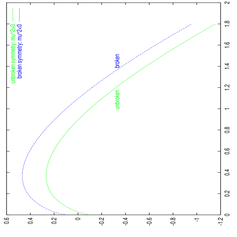
FIG. 2.: The dimensionless scalar field $\varphi^{2}(w)$ as a function of the dimensionless mass $w$ for a coupling $\lambda$ such that ${32\pi^{2}\over\lambda}\;e^{-32\pi^{2}/\lambda}=0.1$. See eq.(12).

FIG. 3.: $\eta(\tau)$ vs. $\tau$. Solid line corresponds to $\eta_{0}=0.03\;;\;\dot{\eta}_{0}=0$, dashed line corresponds to $\eta_{0}=0.1\;;\;\dot{\eta}_{0}=0$, for $g=10^{-7}$.

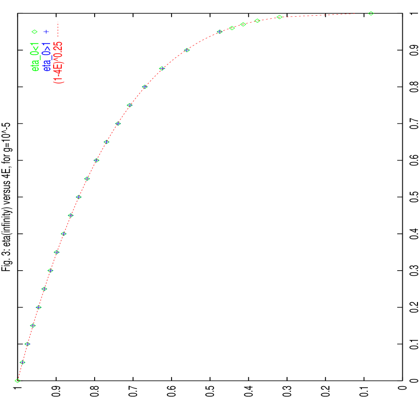
FIG. 4.: $\eta_{\infty}$ as a function of $4E=(\eta_{0}^{2}-1)^{2}$. The points $+$ correspond to $\eta_{0}>1$ whereas the points $\Diamond$ correspond to $\eta_{0}<1$. As discussed in section IV, $\eta_{\infty}$ is invariant under the exchange $\eta_{0}\Leftrightarrow\sqrt{2-\eta_{0}^{2}}$. The continuos curve is $\eta_{\infty}=\left[\eta_{0}^{2}\,(2-\eta_{0}^{2})\right]^{x}$ with $x=0.25$.

FIG. 5.: ${\cal M}^{2}(\tau)$ vs. $\tau$ [see eq.(71)] for $\eta(0)=\dot{\eta}(0)=0$, $g=10^{-7}$

FIG. 6.: ${\cal M}^{2}(\tau)$ as a function of $\tau$ for $g=10^{-5}$ and $\eta_{0}=5$.

FIG. 7.: $\eta(\tau)$ as a function of $\tau$ for $g=10^{-5}$ and $\eta_{0}=5$.

FIG. 8.: $\sqrt{g}|U_{q}(\tau=100)|$ vs. $q$ (see eq.(70) for $\eta(0)=\dot{\eta}(0)=0$, $g=10^{-7}$

FIG. 9.: $\sqrt{g}|U_{q}(\tau=200)|$ vs. $q$ (see eq.(70) for $\eta(0)=\dot{\eta}(0)=0$, $g=10^{-7}$

FIG. 10.: $gr\,C(r,\tau)$ as a function of $r$ for $\tau=25\;;50\;75;\;100$ for $g=10^{-7}$ and $\eta_{0}=\dot{\eta}(0)=0$.

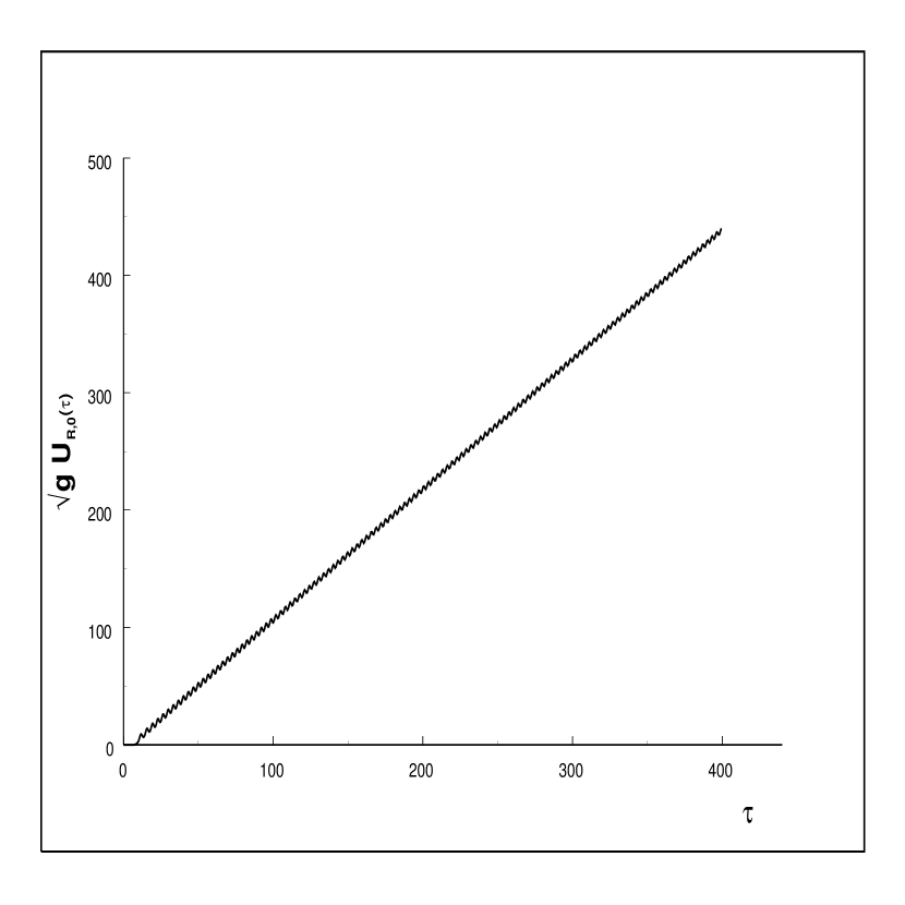
FIG. 11.: $\sqrt{g}U_{R,q=0}(\tau)$ vs. $\tau$ for $\eta(0)=\dot{\eta}(0)=0$, $g=10^{-7}$

FIG. 12.: $\sqrt{g}U_{I,q=0}(\tau)$ vs. $\tau$ for $\eta(0)=\dot{\eta}(0)=0$, $g=10^{-7}$

REFERENCES

- [1] D. Boyanovsky, H. J. de Vega, R. Holman, D.-S. Lee and A. Singh, Phys. Rev. D51, 4419 (1995). D. Boyanovsky, H. J. de Vega and R. Holman, Proceedings of the Second Paris Cosmology Colloquium, Observatoire de Paris, June 1994, pp. 127-215, H. J. de Vega and N. Sánchez, Editors (World Scientific, 1995); Advances in Astrofundamental Physics, Erice Chalonge School, N. Sánchez and A. Zichichi Editors, (World Scientific, 1995).
- [2] D. Boyanovsky, H. J. de Vega and R. Holman, Vth. Erice Chalonge School, Current Topics in Astrofundamental Physics, N. Sánchez and A. Zichichi Editors, World Scientific, 1996, p. 183-270. D. Boyanovsky, M. D’Attanasio, H. J. de Vega, R. Holman and D. S. Lee, Phys. Rev. D52, 6805 (1995).
- [3] F. Cooper, S. Habib, Y. Kluger, E. Mottola, Phys. Rev. D55 (1997), 6471.
- [4] D. Boyanovsky, H. J. de Vega, R. Holman, S. Prem Kumar and R. D. Pisarski, Phys. Rev. D57, 3653 (1998).
- [5] L. Kofman, A. Linde and A. Starobinsky, Phys. Rev. Lett. 73, 3195 (1994) and 76, 1011 (1996). A. Linde, Lectures on Inflationary Cosmology, in Current Topics in Astrofundamental Physics, ‘The Early Universe’, Proceedings of the Chalonge Erice School, N. Sánchez and A. Zichichi Editors, Nato ASI series C, vol. 467, 1995, Kluwer Acad. Publ.
- [6] D. Boyanovsky, H. J. de Vega, R. Holman and J. Salgado, Phys. Rev. D54, 7570 (1996); D. Boyanovsky, D. Cormier, H. J. de Vega, R. Holman, A. Singh, M. Srednicki; Phys. Rev. D56 (1997) 1939.
- [7] E. W. Kolb, A. Riotto and Igor I. Tkachev, Phys. Rev. D56 (1997) 6133; E.W. Kolb, A. Riotto and I.I. Tkachev, Phys. Lett. B423 (1998) 348.
- [8] S. Khlebnikov and I. Tkachev, Phys. Rev. Lett. 77, 219 (1996) and 79, 1607 (1997); I. Tkachev, S. Khlebnikov, L. Kofman, A. Linde, hep-ph/9805209; A. Riotto and I. I. Tkachev Phys.Lett. B385 (1996) 57; I. I. Tkachev, S. Yu. Khlebnikov, I. I. Tkachev, Phys. Lett. B390 (1997) 80.
- [9] S. Kasuya and M. Kawasaki, Phys. Rev. D56, 7597 (1997) and D58 (1998); Phys. Lett. B388, 686 (1996); M. Yamaguchi, J. Yokoyama and M. Kawasaki, Prog. Theor. Phys. 100 (1998) 535.
- [10] J. Baacke, K. Heitmann and C. Paetzold, Phys. Rev. D55 (1997) 7815 and D58 (1998) 125013.
- [11] D. Boyanovsky, H. J. de Vega, C. Destri, R. Holman and J. Salgado, Phys. Rev. D57, 7388 (1998).
- [12] F. Cooper, S. Habib, Y. Kluger, E. Mottola, J. P. Paz, P. R. Anderson, Phys. Rev. D50, 2848 (1994). F. Cooper, Y. Kluger, E. Mottola, J. P. Paz, Phys. Rev. D51, 2377 (1995); F. Cooper and E. Mottola, Mod. Phys. Lett. A 2, 635 (1987); F. Cooper and E. Mottola, Phys. Rev. D36, 3114 (1987); F. Cooper, S.-Y. Pi and P. N. Stancioff, Phys. Rev. D34, 3831 (1986).
- [13] J. Baacke, K. Heitmann and C. Paetzold, Phys. Rev. D57 (1998) 6406; D57 (1998) 6398 and D56 (1997) 6556.
- [14] D. Boyanovsky, H. J. de Vega and R. Holman, Phys. Rev. D 49, 2769 (1994); D. Boyanovsky, D. Cormier, H. J. de Vega, R. Holman et S. Prem Kumar, Phys. Rev. D57, 2166, (1998), (and references therein).
- [15] E. J. Weinberg and A. Wu, Phys. Rev. D36, 2474 (1987).
- [16] D. Boyanovsky and H. J. de Vega, Phys. Rev. D47, 2343 (1993).
- [17] V. Branchina, P. Castorina and D. Zappalà, Phys. Rev. D41, 1948 (1990). A. Ringwald and C. Wetterich, Nucl. Phys. B334, 506 (1990). N. Tetradis and C. Wetterich, Nucl. Phys. B 383, 197 (1992). N. Tetradis and D. Litim, Nucl. Phys. B 464, 492 (1996)
- [18] J. Alexandre, V. Branchina and J. Polonyi, cond-mat/9803007. J. Alexandre, V. Branchina and J. Polonyi, Phys. Rev. D58 (1998) 016002; hep-th/9709060; S.-B. Liao and J. Polonyi, Phys. Rev. D51 (1995) 748.
- [19] N. Tetradis and C. Wetterich, Int.J.Mod.Phys. A9 (1994) 4029; Nucl.Phys. B422 (1994) 541; M. Reuter, N. Tetradis and C. Wetterich, Nucl.Phys. B401 (1993) 567; J. Berges, N. Tetradis, C. Wetterich, Phys.Lett. B393 (1997) 387.
- [20] R. G. Root, Phys. Rev. D 10, 3322 (1974). S. Coleman, R. Jackiw and H. D. Politzer, Phys. Rev. D 10, 2491 (1974).
- [21] L. F. Abbott, J. S. Kang and H. J. Schnitzer, Phys. Rev. D 13, 2212 (1976).
- [22] W. A. Bardeen and M. Moshe, Phys. Rev. D 28, 1372 (1983).
- [23] T. W. B. Kibble, J. Phys. A 9, 1387 (1976).
- [24] M. B. Hindmarsh and T.W.B. Kibble, Rep. Prog. Phys. 58:477 (1995).
- [25] A. Vilenkin and E.P.S. Shellard, ‘Cosmic Strings and other Topological Defects’, Cambridge Monographs on Math. Phys. (Cambridge Univ. Press, 1994).
- [26] W. H. Zurek, Nature 317, 505 (1985); Acta Physica Polonica B24, 1301 1993); Phys. Rep. 276, (1996).
- [27] D. Boyanovsky, D-S. Lee, and A. Singh, Phys. Rev. D48, 800 (1993).
- [28] G.Karra and R.J.Rivers, Phys.Lett. B414 (1997), 28; R.J.Rivers, 3rd. Colloque Cosmologie, Observatoire de Paris, June 1995, p. 341 in the Proceedings edited by H J de Vega and N. Sánchez, World Scientific. A.J. Gill and R.J. Rivers, Phys. Rev. D51 (1995), 6949; G.J. Cheetham, E.J. Copeland, T.S. Evans, R.J. Rivers, Phys. Rev.D47 (1993),5316.
- [29] G. J. Stephens, E. A. Calzetta, B. L. Hu, S. A. Ramsey, Phys. Rev. D59 (1999) 045009. D. Ibaceta and E. Calzetta, hep-ph/9810301 (1998).
- [30] A. J. Bray, Adv. Phys. 43, 357 (1994).
- [31] C. Castellano and M. Zannetti, cond-mat/9807242; C. Castellano, F. Corberi and M. Zannetti, Phys. Rev. E56, 4973 (1997); F. Corberi, A. Coniglio and M. Zannetti, Phys. Rev. E51, 5469 (1995).
- [32] N. Turok and D. N. Spergel, Phys. Rev. Lett. 66, 3093 (1991); D. N. Spergel, N. Turok, W. H. Press and B. S. Ryden, Phys. Rev. D43, 1038 (1991).
- [33] J. A. N. Filipe and A. J. Bray, Phys. Rev. E50, 2523 (1994); J. A. N. Filipe, (Ph. D. Thesis, 1994, unpublished).
- [34] Relaxing the assumption of an instantaneous quench and allowing for a time dependence of the cooling mechanism has been recently studied by M. Bowick and A Momen, Phys. Rev. D58 (1998) 085014.