Bose-Einstein Correlations in a Space-Time Approach to
$e^{+}e^{-}$ Annihilation into Hadrons

Abstract

A new treatment of Bose-Einstein correlations is incorporated in a space-time parton-shower model for $e^{+}e^{-}$ annihilation into hadrons. Two alternative afterburners are discussed, and we use a simple calculable model to demonstrate that they reproduce successfully the size of the hadron emission region. One of the afterburners is used to calculate two-pion correlations in $e^{+}e^{-}\rightarrow Z^{0}\rightarrow hadrons$ and $e^{+}e^{-}\rightarrow W^{+}W^{-}\rightarrow hadrons$. Results are shown with and without resonance decays, for correlations along and transverse to the thrust jet axis in these two classes of events.

1 Introduction

Perturbative parton-shower Monte Carlos [1, 2] combined with models for hadronization provide a very successful description of experimental data on $e^{+}e^{-}\rightarrow Z^{0}\rightarrow hadrons$, deep-inelastic lepton-nucleon scattering, etc.. In most of the applications made so far, attention has been concentrated on distributions and correlations in momentum space. However, there are some key aspects of the physics where better understanding [3] of the space-time development of the hadronic system is desirable [4]. This is particularly true for the treatment of dense hadronic media, such as those produced in heavy-ion collisions, where the formation and expansion of the system are of both experimental and theoretical interest. A prototype for the treatment of such questions may be provided by the reaction $e^{+}e^{-}\rightarrow W^{+}W^{-}\rightarrow hadrons$, where the $W^{\pm}$ do not decay independently, but in a hadronic environment created by each other. This may engender collective effects such as colour reconnection [5, 6, 7, 8], parton exogamy [9, 10] and Bose-Einstein correlations [11, 12, 13] that may be detected by experiment [14, 15, 16], and could be of relevance to the measurement of $m_{W}$ at LEP 2 [17].

A parton-shower Monte Carlo has recently been developed [18] which incorporates the information on the space-time development that is encoded in perturbative QCD [19], and combines it with a phenomenological spatial criterion for confinement [20] to provide a complete space-time description of hadronization. This tool has been applied to the analysis of $e^{+}e^{-}\rightarrow Z^{0}\rightarrow hadrons$ [4], $e^{+}e^{-}\rightarrow W^{+}W^{-}\rightarrow hadrons$ [9, 10], deep-inelastic lepton-nucleon scattering [21] and relativistic heavy-ion collisions [22, 23, 24]. In the application to $e^{+}e^{-}\rightarrow W^{+}W^{-}\rightarrow hadrons$, it has provided new insight into collective effects such as parton ‘exogamy’ [10], namely the marriage of partons from different $W^{\pm}$ parents to produce daughter clusters of final-state hadrons. In the application to relativistic heavy-ion collisions, it has provided useful insights into such issues as the formation and local thermalization of the dense nuclear fireball, hadron production [24], and the possible suppression of the $J/\psi$ [22, 23]. However, little attempt has so far been made to incorporate Bose-Einstein correlations into this space-time model in a realistic way.

Bose-Einstein correlations have been analyzed in many experimental situations, including $e^{+}e^{-}$ annihilation [14, 15] where there has also been considerable recent theoretical progress [25], and have been used extensively as a tool to analyze the hadronic fireballs produced in relativistic heavy-ion collisions [26, 27]. Considerable recent progress has been made in the development of the formalism for analyzing Bose-Einstein correlations [28], and for implementing them in an afterburner for models of hadron production [29, 30, 31]. It was shown that Bose-Einstein correlations in the two-particle momentum spectra allow for a detailed reconstruction [27, 28] of the geometry and dynamical state of the reaction zone from which the final-state hadrons are emitted. The purpose of this paper is to describe the implementation of Bose-Einstein correlations in the space-time parton-shower Monte Carlo mentioned above (see also [32]), and to describe pilot applications to the reactions $e^{+}e^{-}\rightarrow Z^{0}\rightarrow hadrons$ and $e^{+}e^{-}\rightarrow W^{+}W^{-}\rightarrow hadrons$. This work should pave the way for a detailed space-time analysis of hadron production in these reactions using data on two-particle momentum correlations.

We introduce in Section 2 of this paper “classical” and “quantum” algorithms suitable for the calculation of Bose-Einstein correlations in Monte Carlo codes for hadron production. Both algorithms differ in how the numerical event simulation is used to define a quantum mechanical phase space density of emission points. We test these algorithms in Section 3, using a simple and analytically solvable model [33] for the hadron source. We verify that Bose-Einstein analysis tools applied to the hadronic spectra generated by the two versions of the afterburner reproduce correctly the input source geometry. Then, in Section 4 we apply the “quantum” afterburner to hadronic $Z^{0}$ and $W^{+}W^{-}$ final states generated by a parton-shower Monte Carlo. We calculate two-pion correlations with and without resonance decays, studying both the longitudinal and transverse momentum dependences of the correlation functions.

In a final Section, we mention possible future studies using the approach introduced in this paper. These would include implementation of the “classical” version of the Bose-Einstein afterburner, and exploration of the influence on the “quantum” afterburner results of varying the assumed wave-packet size.

2 Bose-Einstein algorithms

In this section we explain the algorithms with which we later calculate two-particle correlations of identical pions from perturbative parton-shower Monte Carlos.

2.1 General considerations

Bose-Einstein correlations reflect the phase-space density of the hadronic source created in the collision. Contrary to single-particle momentum spectra, they thus also provide access to the space-time structure of the reaction zone. A consistent numerical simulation of Bose-Einstein effects on the two-particle and many-particle momentum distributions thus requires by necessity an algorithm which propagates the particles in phase space, rather than in momentum space only. This is what the parton-shower cascade event generator VNI does.

The Bose-Einstein symmetrization effects result in an enhancement at small relative momenta tensysevensyfivesy$\textstyle q$ of the 2-particle coincidence spectrum relative to the product of single particle spectra. The tensysevensyfivesy$\textstyle q$ range of this enhancement is inversely related to the size of the emission region in space-time. All existing shower Monte Carlos, whether formulated in phase space or only in momentum space, are based on a probabilistic description and thus do not correctly describe the many-particle symmetrization effects of the quantum-mechanical time evolution. The corresponding quantum-statistical corrections must therefore be implemented, in some approximation, by an “afterburner” at the end of the classical time evolution.

In momentum-space based Monte Carlos like JETSET, one tries to implement the clustering of identical bosons at small relative momenta by shifting the final state momenta according to certain prescriptions [12, 13]. These shifting prescriptions are not unique and lead to changes in the invariant mass of the particle pair, and thus do not allow one to conserve simultaneously energy and momentum. Furthermore, they involve a weighting function which is put in by hand but should, in principle, reflect the (unknown) space-time structure of the simulated event. A recent attempt to relate the weighting function directly to previously unused information on the space-time structure of the particle-production process is described in [34]. However, its connection to the position of the hadrons at “freeze-out”, i.e., decoupling from the strong interactions, remains at most indirect.

In the present paper, we study two algorithms [29, 30] to implement Bose-Einstein correlations at the end of the Monte Carlo simulation. These algorithms do not shift the particle momenta, nor do they alter the output of the event generator in any other way. They calculate the single-particle inclusive momentum distribution directly from the output momenta of the generator, and the two-particle coincidence spectra from the space-time coordinates and momenta of particle pairs from the generator output. They differ in the way in which they associate with the event generator output a quantum-mechanical Wigner phase space density $S(x,K)$. Both algorithms assume that the particles propagate freely from the source to the detector and include only the quantum-statistical pairwise correlations between identical bosons. Generalizations of these algorithms to include final-state interactions [35] and multiparticle correlation effects [36] have been proposed but not yet implemented numerically.

The two-particle correlation function is constructed as the ratio of the two-particle coincidence spectrum $P_{2}({\leavevmode\mathchoice{\hbox{\rm tensysevensyfivesy\boldmath{$\displaystyle p$}}}{\hbox{\rm tensysevensyfivesy\boldmath{$\textstyle p$}}}{\hbox{\rm tensysevensyfivesy\boldmath{$\scriptstyle p$}}}{\hbox{\rm tensysevensyfivesy\boldmath{$\scriptscriptstyle p$}}}}_{a},{\leavevmode\mathchoice{\hbox{\rm tensysevensyfivesy\boldmath{$\displaystyle p$}}}{\hbox{\rm tensysevensyfivesy\boldmath{$\textstyle p$}}}{\hbox{\rm tensysevensyfivesy\boldmath{$\scriptstyle p$}}}{\hbox{\rm tensysevensyfivesy\boldmath{$\scriptscriptstyle p$}}}}_{b})$ and the product of single-particle inclusive spectra, $P_{1}({\leavevmode\mathchoice{\hbox{\rm tensysevensyfivesy\boldmath{$\displaystyle p$}}}{\hbox{\rm tensysevensyfivesy\boldmath{$\textstyle p$}}}{\hbox{\rm tensysevensyfivesy\boldmath{$\scriptstyle p$}}}{\hbox{\rm tensysevensyfivesy\boldmath{$\scriptscriptstyle p$}}}}_{a,b})$,

$$C({\leavevmode\mathchoice{\hbox{\rm tensysevensyfivesy\boldmath{$\displaystyle q$}}}{\hbox{\rm tensysevensyfivesy\boldmath{$\textstyle q$}}}{\hbox{\rm tensysevensyfivesy\boldmath{$\scriptstyle q$}}}{\hbox{\rm tensysevensyfivesy\boldmath{$\scriptscriptstyle q$}}}},{\leavevmode\mathchoice{\hbox{\rm tensysevensyfivesy\boldmath{$\displaystyle K$}}}{\hbox{\rm tensysevensyfivesy\boldmath{$\textstyle K$}}}{\hbox{\rm tensysevensyfivesy\boldmath{$\scriptstyle K$}}}{\hbox{\rm tensysevensyfivesy\boldmath{$\scriptscriptstyle K$}}}})={\cal N}{P_{2}({\leavevmode\mathchoice{\hbox{\rm tensysevensyfivesy\boldmath{$\displaystyle p$}}}{\hbox{\rm tensysevensyfivesy\boldmath{$\textstyle p$}}}{\hbox{\rm tensysevensyfivesy\boldmath{$\scriptstyle p$}}}{\hbox{\rm tensysevensyfivesy\boldmath{$\scriptscriptstyle p$}}}}_{a},{\leavevmode\mathchoice{\hbox{\rm tensysevensyfivesy\boldmath{$\displaystyle p$}}}{\hbox{\rm tensysevensyfivesy\boldmath{$\textstyle p$}}}{\hbox{\rm tensysevensyfivesy\boldmath{$\scriptstyle p$}}}{\hbox{\rm tensysevensyfivesy\boldmath{$\scriptscriptstyle p$}}}}_{b})\over P_{1}({\leavevmode\mathchoice{\hbox{\rm tensysevensyfivesy\boldmath{$\displaystyle p$}}}{\hbox{\rm tensysevensyfivesy\boldmath{$\textstyle p$}}}{\hbox{\rm tensysevensyfivesy\boldmath{$\scriptstyle p$}}}{\hbox{\rm tensysevensyfivesy\boldmath{$\scriptscriptstyle p$}}}}_{a})\,P_{1}({\leavevmode\mathchoice{\hbox{\rm tensysevensyfivesy\boldmath{$\displaystyle p$}}}{\hbox{\rm tensysevensyfivesy\boldmath{$\textstyle p$}}}{\hbox{\rm tensysevensyfivesy\boldmath{$\scriptstyle p$}}}{\hbox{\rm tensysevensyfivesy\boldmath{$\scriptscriptstyle p$}}}}_{b})}\,,$$ (1)

where ${\leavevmode\mathchoice{\hbox{\rm tensysevensyfivesy\boldmath{$\displaystyle q$}}}{\hbox{\rm tensysevensyfivesy\boldmath{$\textstyle q$}}}{\hbox{\rm tensysevensyfivesy\boldmath{$\scriptstyle q$}}}{\hbox{\rm tensysevensyfivesy\boldmath{$\scriptscriptstyle q$}}}}={\leavevmode\mathchoice{\hbox{\rm tensysevensyfivesy\boldmath{$\displaystyle p$}}}{\hbox{\rm tensysevensyfivesy\boldmath{$\textstyle p$}}}{\hbox{\rm tensysevensyfivesy\boldmath{$\scriptstyle p$}}}{\hbox{\rm tensysevensyfivesy\boldmath{$\scriptscriptstyle p$}}}}_{a}-{\leavevmode\mathchoice{\hbox{\rm tensysevensyfivesy\boldmath{$\displaystyle p$}}}{\hbox{\rm tensysevensyfivesy\boldmath{$\textstyle p$}}}{\hbox{\rm tensysevensyfivesy\boldmath{$\scriptstyle p$}}}{\hbox{\rm tensysevensyfivesy\boldmath{$\scriptscriptstyle p$}}}}_{b}$ is the relative and ${\leavevmode\mathchoice{\hbox{\rm tensysevensyfivesy\boldmath{$\displaystyle K$}}}{\hbox{\rm tensysevensyfivesy\boldmath{$\textstyle K$}}}{\hbox{\rm tensysevensyfivesy\boldmath{$\scriptstyle K$}}}{\hbox{\rm tensysevensyfivesy\boldmath{$\scriptscriptstyle K$}}}}=({\leavevmode\mathchoice{\hbox{\rm tensysevensyfivesy\boldmath{$\displaystyle p$}}}{\hbox{\rm tensysevensyfivesy\boldmath{$\textstyle p$}}}{\hbox{\rm tensysevensyfivesy\boldmath{$\scriptstyle p$}}}{\hbox{\rm tensysevensyfivesy\boldmath{$\scriptscriptstyle p$}}}}_{a}+{\leavevmode\mathchoice{\hbox{\rm tensysevensyfivesy\boldmath{$\displaystyle p$}}}{\hbox{\rm tensysevensyfivesy\boldmath{$\textstyle p$}}}{\hbox{\rm tensysevensyfivesy\boldmath{$\scriptstyle p$}}}{\hbox{\rm tensysevensyfivesy\boldmath{$\scriptscriptstyle p$}}}}_{b})/2$ is the average pair momentum. With the assumption of independent particle emission the two-particle correlation function (1) can then be written as [37, 38, 39, 28]

$$C({\leavevmode\mathchoice{\hbox{\rm tensysevensyfivesy\boldmath{$\displaystyle q$}}}{\hbox{\rm tensysevensyfivesy\boldmath{$\textstyle q$}}}{\hbox{\rm tensysevensyfivesy\boldmath{$\scriptstyle q$}}}{\hbox{\rm tensysevensyfivesy\boldmath{$\scriptscriptstyle q$}}}},{\leavevmode\mathchoice{\hbox{\rm tensysevensyfivesy\boldmath{$\displaystyle K$}}}{\hbox{\rm tensysevensyfivesy\boldmath{$\textstyle K$}}}{\hbox{\rm tensysevensyfivesy\boldmath{$\scriptstyle K$}}}{\hbox{\rm tensysevensyfivesy\boldmath{$\scriptscriptstyle K$}}}})={\cal N}_{s}\left({1+{\left|\int d^{4}x\,S(x,K)\,e^{iq{\cdot}x}\right|^{2}\over\int d^{4}x\,S(x,p_{a})\,\int d^{4}y\,S(y,p_{b})}}\right)\,,$$ (2)

where $S(x,p)$ is the single-particle Wigner phase-space density of the source. In this work we choose the normalization ${\cal N}={\cal N}_{s}=1$ in presenting our results. The implications of other choices of normalization are discussed in Section 2.2. The four-vectors $p_{a,b}$ in the denominator on the r.h.s. are on-shell while the numerator contains the off-shell four-vectors $q$ and $K$ with $q^{0}=E_{a}-E_{b}$ and $K^{0}=(E_{a}+E_{b})/2$. The main question is how to relate the event generator output to this Wigner density, and how to simulate the r.h.s. of Eq. (2). This will be discussed in Section 2.3.

2.2 Normalization of the correlator

The normalization ${\cal N}$ in (1) does not affect the space-time interpretation of the correlator, and the reader who is only interested in the latter can skip the present subsection. The subtle point we discuss here is that, in the context of event generator studies, the normalization ${\cal N}$ of the correlator is only fixed after requiring that the Bose-Einstein algorithm affects the simulated multiplicity in a particular way. We start by recalling the quantum field-theoretical definitions of the single- and two-particle spectra,

$$P_{1}({\leavevmode\mathchoice{\hbox{\rm tensysevensyfivesy\boldmath{$\displaystyle p$}}}{\hbox{\rm tensysevensyfivesy\boldmath{$\textstyle p$}}}{\hbox{\rm tensysevensyfivesy\boldmath{$\scriptstyle p$}}}{\hbox{\rm tensysevensyfivesy\boldmath{$\scriptscriptstyle p$}}}}) = E_{p}\langle{\hat{a}}^{\dagger}_{\leavevmode\mathchoice{\hbox{\rm tensysevensyfivesy\boldmath{$\displaystyle p$}}}{\hbox{\rm tensysevensyfivesy\boldmath{$\textstyle p$}}}{\hbox{\rm tensysevensyfivesy\boldmath{$\scriptstyle p$}}}{\hbox{\rm tensysevensyfivesy\boldmath{$\scriptscriptstyle p$}}}}{\hat{a}}_{\leavevmode\mathchoice{\hbox{\rm tensysevensyfivesy\boldmath{$\displaystyle p$}}}{\hbox{\rm tensysevensyfivesy\boldmath{$\textstyle p$}}}{\hbox{\rm tensysevensyfivesy\boldmath{$\scriptstyle p$}}}{\hbox{\rm tensysevensyfivesy\boldmath{$\scriptscriptstyle p$}}}}\rangle\,,$$ (3)

$$P_{2}({\leavevmode\mathchoice{\hbox{\rm tensysevensyfivesy\boldmath{$\displaystyle p$}}}{\hbox{\rm tensysevensyfivesy\boldmath{$\textstyle p$}}}{\hbox{\rm tensysevensyfivesy\boldmath{$\scriptstyle p$}}}{\hbox{\rm tensysevensyfivesy\boldmath{$\scriptscriptstyle p$}}}}_{a},{\leavevmode\mathchoice{\hbox{\rm tensysevensyfivesy\boldmath{$\displaystyle p$}}}{\hbox{\rm tensysevensyfivesy\boldmath{$\textstyle p$}}}{\hbox{\rm tensysevensyfivesy\boldmath{$\scriptstyle p$}}}{\hbox{\rm tensysevensyfivesy\boldmath{$\scriptscriptstyle p$}}}}_{b}) = E_{a}\,E_{b}\,\langle{\hat{a}}^{\dagger}_{{\leavevmode\mathchoice{\hbox{\rm tensysevensyfivesy\boldmath{$\displaystyle p$}}}{\hbox{\rm tensysevensyfivesy\boldmath{$\textstyle p$}}}{\hbox{\rm tensysevensyfivesy\boldmath{$\scriptstyle p$}}}{\hbox{\rm tensysevensyfivesy\boldmath{$\scriptscriptstyle p$}}}}_{a}}{\hat{a}}^{\dagger}_{{\leavevmode\mathchoice{\hbox{\rm tensysevensyfivesy\boldmath{$\displaystyle p$}}}{\hbox{\rm tensysevensyfivesy\boldmath{$\textstyle p$}}}{\hbox{\rm tensysevensyfivesy\boldmath{$\scriptstyle p$}}}{\hbox{\rm tensysevensyfivesy\boldmath{$\scriptscriptstyle p$}}}}_{b}}{\hat{a}}_{{\leavevmode\mathchoice{\hbox{\rm tensysevensyfivesy\boldmath{$\displaystyle p$}}}{\hbox{\rm tensysevensyfivesy\boldmath{$\textstyle p$}}}{\hbox{\rm tensysevensyfivesy\boldmath{$\scriptstyle p$}}}{\hbox{\rm tensysevensyfivesy\boldmath{$\scriptscriptstyle p$}}}}_{b}}{\hat{a}}_{{\leavevmode\mathchoice{\hbox{\rm tensysevensyfivesy\boldmath{$\displaystyle p$}}}{\hbox{\rm tensysevensyfivesy\boldmath{$\textstyle p$}}}{\hbox{\rm tensysevensyfivesy\boldmath{$\scriptstyle p$}}}{\hbox{\rm tensysevensyfivesy\boldmath{$\scriptscriptstyle p$}}}}_{a}}\rangle\,,$$ (4)

where $\langle...\rangle$ indicates the ensemble of physical states (events) for which the correlator is calculated. This implies the normalizations

$$\int P_{1}({\leavevmode\mathchoice{\hbox{\rm tensysevensyfivesy\boldmath{$\displaystyle p$}}}{\hbox{\rm tensysevensyfivesy\boldmath{$\textstyle p$}}}{\hbox{\rm tensysevensyfivesy\boldmath{$\scriptstyle p$}}}{\hbox{\rm tensysevensyfivesy\boldmath{$\scriptscriptstyle p$}}}})\,{d^{3}p\over E_{p}} = \langle{\hat{N}}\rangle\,,$$ (5)

$$\int P_{2}({\leavevmode\mathchoice{\hbox{\rm tensysevensyfivesy\boldmath{$\displaystyle p$}}}{\hbox{\rm tensysevensyfivesy\boldmath{$\textstyle p$}}}{\hbox{\rm tensysevensyfivesy\boldmath{$\scriptstyle p$}}}{\hbox{\rm tensysevensyfivesy\boldmath{$\scriptscriptstyle p$}}}}_{a},{\leavevmode\mathchoice{\hbox{\rm tensysevensyfivesy\boldmath{$\displaystyle p$}}}{\hbox{\rm tensysevensyfivesy\boldmath{$\textstyle p$}}}{\hbox{\rm tensysevensyfivesy\boldmath{$\scriptstyle p$}}}{\hbox{\rm tensysevensyfivesy\boldmath{$\scriptscriptstyle p$}}}}_{b})\,{d^{3}p_{a}\over E_{a}}\,{d^{3}p_{b}\over E_{b}} = \langle{\hat{N}}({\hat{N}}-1)\rangle\,,$$ (6)

where ${\hat{N}}=\int(d^{3}p/E)\,{\hat{a}}^{\dagger}_{\leavevmode\mathchoice{\hbox{\rm tensysevensyfivesy\boldmath{$\displaystyle p$}}}{\hbox{\rm tensysevensyfivesy\boldmath{$\textstyle p$}}}{\hbox{\rm tensysevensyfivesy\boldmath{$\scriptstyle p$}}}{\hbox{\rm tensysevensyfivesy\boldmath{$\scriptscriptstyle p$}}}}{\hat{a}}_{\leavevmode\mathchoice{\hbox{\rm tensysevensyfivesy\boldmath{$\displaystyle p$}}}{\hbox{\rm tensysevensyfivesy\boldmath{$\textstyle p$}}}{\hbox{\rm tensysevensyfivesy\boldmath{$\scriptstyle p$}}}{\hbox{\rm tensysevensyfivesy\boldmath{$\scriptscriptstyle p$}}}}$ is the particle number operator. We now discuss the physical implications of two different normalizations of the correlator:

1. One can interpret the two-particle correlator as a factor [13]

   $$d^{6}\sigma_{\pi\pi}^{\rm BE}/d^{3}{\leavevmode\mathchoice{\hbox{\rm tensysevensyfivesy\boldmath{$\displaystyle p$}}}{\hbox{\rm tensysevensyfivesy\boldmath{$\textstyle p$}}}{\hbox{\rm tensysevensyfivesy\boldmath{$\scriptstyle p$}}}{\hbox{\rm tensysevensyfivesy\boldmath{$\scriptscriptstyle p$}}}}_{1}\,d^{3}{\leavevmode\mathchoice{\hbox{\rm tensysevensyfivesy\boldmath{$\displaystyle p$}}}{\hbox{\rm tensysevensyfivesy\boldmath{$\textstyle p$}}}{\hbox{\rm tensysevensyfivesy\boldmath{$\scriptstyle p$}}}{\hbox{\rm tensysevensyfivesy\boldmath{$\scriptscriptstyle p$}}}}_{2}=C({\leavevmode\mathchoice{\hbox{\rm tensysevensyfivesy\boldmath{$\displaystyle q$}}}{\hbox{\rm tensysevensyfivesy\boldmath{$\textstyle q$}}}{\hbox{\rm tensysevensyfivesy\boldmath{$\scriptstyle q$}}}{\hbox{\rm tensysevensyfivesy\boldmath{$\scriptscriptstyle q$}}}},{\leavevmode\mathchoice{\hbox{\rm tensysevensyfivesy\boldmath{$\displaystyle K$}}}{\hbox{\rm tensysevensyfivesy\boldmath{$\textstyle K$}}}{\hbox{\rm tensysevensyfivesy\boldmath{$\scriptstyle K$}}}{\hbox{\rm tensysevensyfivesy\boldmath{$\scriptscriptstyle K$}}}})\,d^{6}\sigma_{\pi\pi}^{\rm NO}/d^{3}{\leavevmode\mathchoice{\hbox{\rm tensysevensyfivesy\boldmath{$\displaystyle p$}}}{\hbox{\rm tensysevensyfivesy\boldmath{$\textstyle p$}}}{\hbox{\rm tensysevensyfivesy\boldmath{$\scriptstyle p$}}}{\hbox{\rm tensysevensyfivesy\boldmath{$\scriptscriptstyle p$}}}}_{1}\,d^{3}{\leavevmode\mathchoice{\hbox{\rm tensysevensyfivesy\boldmath{$\displaystyle p$}}}{\hbox{\rm tensysevensyfivesy\boldmath{$\textstyle p$}}}{\hbox{\rm tensysevensyfivesy\boldmath{$\scriptstyle p$}}}{\hbox{\rm tensysevensyfivesy\boldmath{$\scriptscriptstyle p$}}}}_{2}$$ (7)

   relating the measured two-particle differential cross sections on the l.h.s. to the differential two-particle cross section resulting from the simulation. Requiring that the Bose-Einstein afterburner conserves event multiplicities on an event-by-event level, the corresponding momentum integrated total two-particle cross sections have to coincide, $\sigma_{\pi\pi}^{\rm BE}=\sigma_{\pi\pi}^{\rm NO}$. This is the appropriate starting point if total pair cross sections are used in the tuning of the event generator which then, of course, should not be changed by the Bose-Einstein afterburner. The normalization satisfying these requirements normalizes both the numerator and denominator of (1) separately to unity [40],

   $${\cal N}={{\langle\hat{N}\rangle}^{2}\over{\langle\hat{N}(\hat{N}-1)}\rangle}\,.$$ (8)

   This results in a normalization ${\cal N}_{s}<1$ of the two-particle correlator (2) [41, 36, 42].

2. A different choice of normalization often used in heavy-ion physics is [28]

   $${\cal N}={\cal N}_{s}=1\,.$$ (9)

   Combining (1) and (2), it follows that

   $$P_{2}({\leavevmode\mathchoice{\hbox{\rm tensysevensyfivesy\boldmath{$\displaystyle p$}}}{\hbox{\rm tensysevensyfivesy\boldmath{$\textstyle p$}}}{\hbox{\rm tensysevensyfivesy\boldmath{$\scriptstyle p$}}}{\hbox{\rm tensysevensyfivesy\boldmath{$\scriptscriptstyle p$}}}}_{a},{\leavevmode\mathchoice{\hbox{\rm tensysevensyfivesy\boldmath{$\displaystyle p$}}}{\hbox{\rm tensysevensyfivesy\boldmath{$\textstyle p$}}}{\hbox{\rm tensysevensyfivesy\boldmath{$\scriptstyle p$}}}{\hbox{\rm tensysevensyfivesy\boldmath{$\scriptscriptstyle p$}}}}_{b})=E_{a}\,E_{b}{d^{6}N\over d^{3}p_{a}\,d^{3}p_{b}}>P_{1}({\leavevmode\mathchoice{\hbox{\rm tensysevensyfivesy\boldmath{$\displaystyle p$}}}{\hbox{\rm tensysevensyfivesy\boldmath{$\textstyle p$}}}{\hbox{\rm tensysevensyfivesy\boldmath{$\scriptstyle p$}}}{\hbox{\rm tensysevensyfivesy\boldmath{$\scriptscriptstyle p$}}}}_{a})\,P_{1}({\leavevmode\mathchoice{\hbox{\rm tensysevensyfivesy\boldmath{$\displaystyle p$}}}{\hbox{\rm tensysevensyfivesy\boldmath{$\textstyle p$}}}{\hbox{\rm tensysevensyfivesy\boldmath{$\scriptstyle p$}}}{\hbox{\rm tensysevensyfivesy\boldmath{$\scriptscriptstyle p$}}}}_{b})=\left(E_{a}{d^{3}N\over d^{3}p_{a}}\right)\left(E_{b}{d^{3}N\over d^{3}p_{b}}\right)\,,$$ (10)

   and, because of (5,6), also that

   $$\langle{\hat{N}}({\hat{N}}-1)\rangle>\langle{\hat{N}}\rangle^{2}\,.$$ (11)

   If we interpret the r.h.s. of these equations as the pair spectra and pair multiplicity from the event generator, implying that the generated multiplicity has a Poisson distribution, ($\langle N(N-1)\rangle_{\rm gen}=\langle N\rangle^{2}_{\rm gen}$, then this implies that the Bose-Einstein effects have increased the pair multiplicity. This may account for some of the effects of Bose-Einstein statistics on the particle-production processes prior to freeze-out [43].

Depending whether we require for the Bose-Einstein afterburner the conservation of event multiplicities on an event-by-event level, or aim to mimic Bose-Einstein effects during the particle-production processes as well, the normalization of the two-particle correlator is thus either smaller than unity or unity itself. In the present paper, we are only investigating the space-time interpretation of the two-particle correlator, and hence we can set ${\cal N}={\cal N}_{s}=1$ without any loss of generality.

2.3 Wigner densities and event generator output

We now explain how we construct a two-particle spectrum with the properties (9-11) from the event generator output. For simplicity, we discuss only one particle species, say $\pi^{+}$. The event generator yields for each collision event $m$ a set of final (on-shell) $\pi^{+}$ momenta $p_{i}=(E_{i},{\leavevmode\mathchoice{\hbox{\rm tensysevensyfivesy\boldmath{$\displaystyle p$}}}{\hbox{\rm tensysevensyfivesy\boldmath{$\textstyle p$}}}{\hbox{\rm tensysevensyfivesy\boldmath{$\scriptstyle p$}}}{\hbox{\rm tensysevensyfivesy\boldmath{$\scriptscriptstyle p$}}}}_{i})$ and last interaction points $r_{i}=(t_{i},\leavevmode\mathchoice{\hbox{\rm tensysevensyfivesy\boldmath{$\displaystyle r$}}}{\hbox{\rm tensysevensyfivesy\boldmath{$\textstyle r$}}}{\hbox{\rm tensysevensyfivesy\boldmath{$\scriptstyle r$}}}{\hbox{\rm tensysevensyfivesy\boldmath{$\scriptscriptstyle r$}}}_{i})$, with $i=1,2,\dots,N_{m}$ where $N_{m}$ is the total number of $\pi^{+}$ created in event $m$:

$$\{(r_{i},p_{i})\,|\,i=1,2,\dots,N_{m}\}.$$ (12)

They define a classical (positive definite) phase-space density

$$\rho_{\rm class}(x,p)={1\over N_{\rm evt}}\sum_{m=1}^{N_{\rm evt}}\rho^{(m)}_{\rm class}(x,p)={1\over N_{\rm evt}}\sum_{m=1}^{N_{\rm evt}}\sum_{i=1}^{N_{m}}\delta^{(4)}(x-r_{i})\,\delta^{(4)}(p-p_{i})\,.$$ (13)

The distributions $\rho^{(m)}_{\rm class}(x,p)$ for individual events cannot be taken as Wigner densities since they fix the particle coordinates and momenta simultaneously, thereby violating the uncertainty relation. This can affect the calculation of the two-particle correlator significantly [31]. Furthermore, $\rho_{\rm class}(x,p)$ is always positive, whilst the Wigner density $S(x,p)$ can, at least in principle, become negative. Only when averaged over sufficiently large phase-space regions is the latter guaranteed to be positive definite. On the other hand, it is unlikely that such Zitterbewegung oscillations of $S(x,p)$ or the spiky structure of $\rho_{\rm class}(x,p)$ affect the correlation function at small tensysevensyfivesy$\textstyle q$ where the Bose-Einstein effects become visible. It is well known [28] that the width of the correlation function reflects only the r.m.s. width of the Wigner density $S(x,p)$ in coordinate space, and that finer structures in $S(x,p)$ (like spikes or quantum oscillations) show up in the correlator only at large tensysevensyfivesy$\textstyle q$ and are very hard to resolve experimentally. Furthermore, since the event generator performs a Monte Carlo simulation of a dynamical evolution which is based on quantum-mechanical transition amplitudes, averaging its output over many simulated events should generate a smooth phase-space distribution (13) which is not in conflict with the uncertainty relation.

Following these arguments, one can try to identify directly the classical phase-space density $\rho_{\rm class}(x,p)$ (13), averaged over sufficiently many events, with the on-shell source Wigner density $S(x,p)$ in (2), in the following sense:

$$\rho_{\rm class}(x,p)=2\theta(p^{0})\,\delta(p^{2}-m^{2})S(x,p)\,.$$ (14)

This ensures the correct normalization to the average multiplicity $\langle N\rangle$:

$$\int{d^{3}p\over E_{p}}\,\int d^{4}x\,S(x;{\leavevmode\mathchoice{\hbox{\rm tensysevensyfivesy\boldmath{$\displaystyle p$}}}{\hbox{\rm tensysevensyfivesy\boldmath{$\textstyle p$}}}{\hbox{\rm tensysevensyfivesy\boldmath{$\scriptstyle p$}}}{\hbox{\rm tensysevensyfivesy\boldmath{$\scriptscriptstyle p$}}}},E_{p})=\int d^{4}p\,d^{4}x\,\rho_{\rm class}(x,p)={1\over N_{\rm evt}}\sum_{m=1}^{N_{\rm evt}}N_{m}=\langle N\rangle\,.$$ (15)

The identification (14) gives rise to the “classical” version of our Bose-Einstein afterburner [29], to be discussed in Sec. 2.3.1.

Alternatively, if one wants to avoid the conceptual difficulty of relating an expression like (13), where every term under the sum explicitly violates the uncertainty relation, with the source Wigner density, one can associate the set of phase space points (12) with the phase-space locations of the centers of minimum-uncertainty wave packets [30]:

$$(\leavevmode\mathchoice{\hbox{\rm tensysevensyfivesy\boldmath{$\displaystyle r$}}}{\hbox{\rm tensysevensyfivesy\boldmath{$\textstyle r$}}}{\hbox{\rm tensysevensyfivesy\boldmath{$\scriptstyle r$}}}{\hbox{\rm tensysevensyfivesy\boldmath{$\scriptscriptstyle r$}}}_{i},\leavevmode\mathchoice{\hbox{\rm tensysevensyfivesy\boldmath{$\displaystyle p$}}}{\hbox{\rm tensysevensyfivesy\boldmath{$\textstyle p$}}}{\hbox{\rm tensysevensyfivesy\boldmath{$\scriptstyle p$}}}{\hbox{\rm tensysevensyfivesy\boldmath{$\scriptscriptstyle p$}}}_{i},{t}_{i})\longrightarrow f_{i}(\leavevmode\mathchoice{\hbox{\rm tensysevensyfivesy\boldmath{$\displaystyle x$}}}{\hbox{\rm tensysevensyfivesy\boldmath{$\textstyle x$}}}{\hbox{\rm tensysevensyfivesy\boldmath{$\scriptstyle x$}}}{\hbox{\rm tensysevensyfivesy\boldmath{$\scriptscriptstyle x$}}},{t}_{i})={1\over(\pi\sigma^{2})^{3/4}}\,e^{-(\leavevmode\mathchoice{\hbox{\rm tensysevensyfivesy\boldmath{$\displaystyle x$}}}{\hbox{\rm tensysevensyfivesy\boldmath{$\textstyle x$}}}{\hbox{\rm tensysevensyfivesy\boldmath{$\scriptstyle x$}}}{\hbox{\rm tensysevensyfivesy\boldmath{$\scriptscriptstyle x$}}}-\leavevmode\mathchoice{\hbox{\rm tensysevensyfivesy\boldmath{$\displaystyle r$}}}{\hbox{\rm tensysevensyfivesy\boldmath{$\textstyle r$}}}{\hbox{\rm tensysevensyfivesy\boldmath{$\scriptstyle r$}}}{\hbox{\rm tensysevensyfivesy\boldmath{$\scriptscriptstyle r$}}}_{i})^{2}/(2\sigma^{2})+i\leavevmode\mathchoice{\hbox{\rm tensysevensyfivesy\boldmath{$\displaystyle p$}}}{\hbox{\rm tensysevensyfivesy\boldmath{$\textstyle p$}}}{\hbox{\rm tensysevensyfivesy\boldmath{$\scriptstyle p$}}}{\hbox{\rm tensysevensyfivesy\boldmath{$\scriptscriptstyle p$}}}_{i}\cdot\leavevmode\mathchoice{\hbox{\rm tensysevensyfivesy\boldmath{$\displaystyle x$}}}{\hbox{\rm tensysevensyfivesy\boldmath{$\textstyle x$}}}{\hbox{\rm tensysevensyfivesy\boldmath{$\scriptstyle x$}}}{\hbox{\rm tensysevensyfivesy\boldmath{$\scriptscriptstyle x$}}}}\,.$$ (16)

In this case one enforces quantum-mechanical consistency of the emission function $S(x,p)$ at the level of each individual simulated event. The identification (16) gives rise to the “quantum” version of our Bose-Einstein afterburner [29, 30], to be discussed in Sec. 2.3.2. The word “quantum” in this case stresses the quantum-mechanical consistency of the Wigner density on the event-by-event level (which may indeed be requiring too much), while the “classical” algorithm generates a quantum-mechanically consistent emission function only on the ensemble level, and only if $\rho_{\rm class}$ does not violate the uncertainty relation (see Sec. 3).

Before turning to a discussion of these two algorithms we shortly comment on the underlying assumptions. The use of single-particle Wigner densities $S(x,p)$ implies that the $N$-particle production amplitude factorizes into one-particle production amplitudes [44, 28]. In general, $P_{2}({\leavevmode\mathchoice{\hbox{\rm tensysevensyfivesy\boldmath{$\displaystyle p$}}}{\hbox{\rm tensysevensyfivesy\boldmath{$\textstyle p$}}}{\hbox{\rm tensysevensyfivesy\boldmath{$\scriptstyle p$}}}{\hbox{\rm tensysevensyfivesy\boldmath{$\scriptscriptstyle p$}}}}_{a},{\leavevmode\mathchoice{\hbox{\rm tensysevensyfivesy\boldmath{$\displaystyle p$}}}{\hbox{\rm tensysevensyfivesy\boldmath{$\textstyle p$}}}{\hbox{\rm tensysevensyfivesy\boldmath{$\scriptstyle p$}}}{\hbox{\rm tensysevensyfivesy\boldmath{$\scriptscriptstyle p$}}}}_{b})$ is given by a sum over the two possible permutations of the Fourier transform of the quantum mechanical two-particle Wigner density $S_{2}(x_{a},p_{a};x_{b},p_{b})$ of the source at freeze-out [45]; here we assume $S_{2}(x_{a},p_{a};x_{b},p_{b})=S(x_{a},p_{a})\,S(x_{b},p_{b})$. This assumption (which amounts to a Wick decomposition of the r.h.s. of (4) [28]) implies that the two particles in the pair are emitted independently from each other. It thus neglects dynamical correlations between the two particles in the pair, due, e.g., to energy-momentum conservation, as well as certain quantum-statistical correlations which may be induced on the two-particle level by the symmetry of the multi-particle final-state wave function. While the neglect of dynamical correlations is probably well justified for heavy-ion collisions for which our algorithms were developed [29, 30], the same is much less obvious for $e^{+}e^{-}$ collisions. At high energies, however, we expect such dynamical correlations to affect the two-particle spectrum mostly at large values of tensysevensyfivesy$\textstyle q$, where kinematical constraints play an important role, and not to interfere with the Bose-Einstein correlations at small tensysevensyfivesy$\textstyle q$. If this is true, they cancel from the ratio (1) as constructed by our algorithm (see below). Multi-particle symmetrization effects, on the other hand, are more of an issue in heavy-ion physics [36, 46] where the rapidity densities of the produced particles are large, while their neglect in $e^{+}e^{-}$ collisions seems unproblematic. Furthermore, it is known [42] that for certain classes of multiplicity distributions they do not destroy the factorization of the two-particle Wigner density which is assumed here.

2.3.1 “Classical” version of the Bose-Einstein afterburner

We start from (13) and (14). The momenta returned from the event generator are on-shell, and we hence write from now on $S(x,{\leavevmode\mathchoice{\hbox{\rm tensysevensyfivesy\boldmath{$\displaystyle p$}}}{\hbox{\rm tensysevensyfivesy\boldmath{$\textstyle p$}}}{\hbox{\rm tensysevensyfivesy\boldmath{$\scriptstyle p$}}}{\hbox{\rm tensysevensyfivesy\boldmath{$\scriptscriptstyle p$}}}})$ respectively $\rho_{\rm class}(x,{\leavevmode\mathchoice{\hbox{\rm tensysevensyfivesy\boldmath{$\displaystyle p$}}}{\hbox{\rm tensysevensyfivesy\boldmath{$\textstyle p$}}}{\hbox{\rm tensysevensyfivesy\boldmath{$\scriptstyle p$}}}{\hbox{\rm tensysevensyfivesy\boldmath{$\scriptscriptstyle p$}}}})$ for the on-shell distributions. The $\delta$-function structure of $\rho_{\rm class}$ requires one in practice to bin in the momentum variable (since the $x$-dependence is integrated over in (2), no binning in $x$ is necessary there). For this purpose we introduce the normalized “bin functions” with bin width $\epsilon$

$$\delta^{(\epsilon)}_{{\leavevmode\mathchoice{\hbox{\rm tensysevensyfivesy\boldmath{$\displaystyle p$}}}{\hbox{\rm tensysevensyfivesy\boldmath{$\textstyle p$}}}{\hbox{\rm tensysevensyfivesy\boldmath{$\scriptstyle p$}}}{\hbox{\rm tensysevensyfivesy\boldmath{$\scriptscriptstyle p$}}}}_{i},{\leavevmode\mathchoice{\hbox{\rm tensysevensyfivesy\boldmath{$\displaystyle p$}}}{\hbox{\rm tensysevensyfivesy\boldmath{$\textstyle p$}}}{\hbox{\rm tensysevensyfivesy\boldmath{$\scriptstyle p$}}}{\hbox{\rm tensysevensyfivesy\boldmath{$\scriptscriptstyle p$}}}}}=\left\{\begin{array}[]{r@{\quad:\quad}l}1/\epsilon^{3}&p_{j}-{\epsilon\over 2}\leq p_{i,j}\leq p_{j}+{\epsilon\over 2}\qquad(j=x,y,z)\\ 0&{\rm otherwise}\end{array}\right.$$ (17)

or, alternatively, properly normalized Gaussians of width $\epsilon$,

$$\delta^{(\epsilon)}_{{\leavevmode\mathchoice{\hbox{\rm tensysevensyfivesy\boldmath{$\displaystyle p$}}}{\hbox{\rm tensysevensyfivesy\boldmath{$\textstyle p$}}}{\hbox{\rm tensysevensyfivesy\boldmath{$\scriptstyle p$}}}{\hbox{\rm tensysevensyfivesy\boldmath{$\scriptscriptstyle p$}}}}_{i},{\leavevmode\mathchoice{\hbox{\rm tensysevensyfivesy\boldmath{$\displaystyle p$}}}{\hbox{\rm tensysevensyfivesy\boldmath{$\textstyle p$}}}{\hbox{\rm tensysevensyfivesy\boldmath{$\scriptstyle p$}}}{\hbox{\rm tensysevensyfivesy\boldmath{$\scriptscriptstyle p$}}}}}={1\over(\pi\epsilon^{2})^{3/2}}\exp\left(-({\leavevmode\mathchoice{\hbox{\rm tensysevensyfivesy\boldmath{$\displaystyle p$}}}{\hbox{\rm tensysevensyfivesy\boldmath{$\textstyle p$}}}{\hbox{\rm tensysevensyfivesy\boldmath{$\scriptstyle p$}}}{\hbox{\rm tensysevensyfivesy\boldmath{$\scriptscriptstyle p$}}}}_{i}-{\leavevmode\mathchoice{\hbox{\rm tensysevensyfivesy\boldmath{$\displaystyle p$}}}{\hbox{\rm tensysevensyfivesy\boldmath{$\textstyle p$}}}{\hbox{\rm tensysevensyfivesy\boldmath{$\scriptstyle p$}}}{\hbox{\rm tensysevensyfivesy\boldmath{$\scriptscriptstyle p$}}}})^{2}/\epsilon^{2}\right)\,.$$ (18)

In the limit $\epsilon\to 0$, these Gaussian bin functions reduce to the properly normalized $\delta$ functions $\delta^{(3)}({\leavevmode\mathchoice{\hbox{\rm tensysevensyfivesy\boldmath{$\displaystyle p$}}}{\hbox{\rm tensysevensyfivesy\boldmath{$\textstyle p$}}}{\hbox{\rm tensysevensyfivesy\boldmath{$\scriptstyle p$}}}{\hbox{\rm tensysevensyfivesy\boldmath{$\scriptscriptstyle p$}}}}_{i}-{\leavevmode\mathchoice{\hbox{\rm tensysevensyfivesy\boldmath{$\displaystyle p$}}}{\hbox{\rm tensysevensyfivesy\boldmath{$\textstyle p$}}}{\hbox{\rm tensysevensyfivesy\boldmath{$\scriptstyle p$}}}{\hbox{\rm tensysevensyfivesy\boldmath{$\scriptscriptstyle p$}}}})$. For each event $m$ we calculate the numerator and denominator of (7) separately. We find for the invariant two-particle spectrum in the numerator [29]

$$P_{2}({\leavevmode\mathchoice{\hbox{\rm tensysevensyfivesy\boldmath{$\displaystyle p$}}}{\hbox{\rm tensysevensyfivesy\boldmath{$\textstyle p$}}}{\hbox{\rm tensysevensyfivesy\boldmath{$\scriptstyle p$}}}{\hbox{\rm tensysevensyfivesy\boldmath{$\scriptscriptstyle p$}}}}_{a},{\leavevmode\mathchoice{\hbox{\rm tensysevensyfivesy\boldmath{$\displaystyle p$}}}{\hbox{\rm tensysevensyfivesy\boldmath{$\textstyle p$}}}{\hbox{\rm tensysevensyfivesy\boldmath{$\scriptstyle p$}}}{\hbox{\rm tensysevensyfivesy\boldmath{$\scriptscriptstyle p$}}}}_{b})=E_{a}\,E_{b}\sum_{i\neq j}^{N_{m}}\left(\delta^{(\epsilon)}_{{\leavevmode\mathchoice{\hbox{\rm tensysevensyfivesy\boldmath{$\displaystyle p$}}}{\hbox{\rm tensysevensyfivesy\boldmath{$\textstyle p$}}}{\hbox{\rm tensysevensyfivesy\boldmath{$\scriptstyle p$}}}{\hbox{\rm tensysevensyfivesy\boldmath{$\scriptscriptstyle p$}}}}_{i},{\leavevmode\mathchoice{\hbox{\rm tensysevensyfivesy\boldmath{$\displaystyle p$}}}{\hbox{\rm tensysevensyfivesy\boldmath{$\textstyle p$}}}{\hbox{\rm tensysevensyfivesy\boldmath{$\scriptstyle p$}}}{\hbox{\rm tensysevensyfivesy\boldmath{$\scriptscriptstyle p$}}}}_{a}}\,\delta^{(\epsilon)}_{{\leavevmode\mathchoice{\hbox{\rm tensysevensyfivesy\boldmath{$\displaystyle p$}}}{\hbox{\rm tensysevensyfivesy\boldmath{$\textstyle p$}}}{\hbox{\rm tensysevensyfivesy\boldmath{$\scriptstyle p$}}}{\hbox{\rm tensysevensyfivesy\boldmath{$\scriptscriptstyle p$}}}}_{j},{\leavevmode\mathchoice{\hbox{\rm tensysevensyfivesy\boldmath{$\displaystyle p$}}}{\hbox{\rm tensysevensyfivesy\boldmath{$\textstyle p$}}}{\hbox{\rm tensysevensyfivesy\boldmath{$\scriptstyle p$}}}{\hbox{\rm tensysevensyfivesy\boldmath{$\scriptscriptstyle p$}}}}_{b}}+\delta^{(\epsilon)}_{{\leavevmode\mathchoice{\hbox{\rm tensysevensyfivesy\boldmath{$\displaystyle p$}}}{\hbox{\rm tensysevensyfivesy\boldmath{$\textstyle p$}}}{\hbox{\rm tensysevensyfivesy\boldmath{$\scriptstyle p$}}}{\hbox{\rm tensysevensyfivesy\boldmath{$\scriptscriptstyle p$}}}}_{i},{\leavevmode\mathchoice{\hbox{\rm tensysevensyfivesy\boldmath{$\displaystyle K$}}}{\hbox{\rm tensysevensyfivesy\boldmath{$\textstyle K$}}}{\hbox{\rm tensysevensyfivesy\boldmath{$\scriptstyle K$}}}{\hbox{\rm tensysevensyfivesy\boldmath{$\scriptscriptstyle K$}}}}}\,\delta^{(\epsilon)}_{{\leavevmode\mathchoice{\hbox{\rm tensysevensyfivesy\boldmath{$\displaystyle p$}}}{\hbox{\rm tensysevensyfivesy\boldmath{$\textstyle p$}}}{\hbox{\rm tensysevensyfivesy\boldmath{$\scriptstyle p$}}}{\hbox{\rm tensysevensyfivesy\boldmath{$\scriptscriptstyle p$}}}}_{j},{\leavevmode\mathchoice{\hbox{\rm tensysevensyfivesy\boldmath{$\displaystyle K$}}}{\hbox{\rm tensysevensyfivesy\boldmath{$\textstyle K$}}}{\hbox{\rm tensysevensyfivesy\boldmath{$\scriptstyle K$}}}{\hbox{\rm tensysevensyfivesy\boldmath{$\scriptscriptstyle K$}}}}}\cos(q\cdot(r_{i}-r_{j}))\right)$$ (19)

and for the product of single-particle spectra in the denominator

$$P_{1}({\leavevmode\mathchoice{\hbox{\rm tensysevensyfivesy\boldmath{$\displaystyle p$}}}{\hbox{\rm tensysevensyfivesy\boldmath{$\textstyle p$}}}{\hbox{\rm tensysevensyfivesy\boldmath{$\scriptstyle p$}}}{\hbox{\rm tensysevensyfivesy\boldmath{$\scriptscriptstyle p$}}}}_{a})\,P_{1}({\leavevmode\mathchoice{\hbox{\rm tensysevensyfivesy\boldmath{$\displaystyle p$}}}{\hbox{\rm tensysevensyfivesy\boldmath{$\textstyle p$}}}{\hbox{\rm tensysevensyfivesy\boldmath{$\scriptstyle p$}}}{\hbox{\rm tensysevensyfivesy\boldmath{$\scriptscriptstyle p$}}}}_{b})=E_{a}\,E_{b}\sum_{i\neq j}^{N_{m}}\sum_{j}^{N_{m}}\delta^{(\epsilon)}_{{\leavevmode\mathchoice{\hbox{\rm tensysevensyfivesy\boldmath{$\displaystyle p$}}}{\hbox{\rm tensysevensyfivesy\boldmath{$\textstyle p$}}}{\hbox{\rm tensysevensyfivesy\boldmath{$\scriptstyle p$}}}{\hbox{\rm tensysevensyfivesy\boldmath{$\scriptscriptstyle p$}}}}_{i},{\leavevmode\mathchoice{\hbox{\rm tensysevensyfivesy\boldmath{$\displaystyle p$}}}{\hbox{\rm tensysevensyfivesy\boldmath{$\textstyle p$}}}{\hbox{\rm tensysevensyfivesy\boldmath{$\scriptstyle p$}}}{\hbox{\rm tensysevensyfivesy\boldmath{$\scriptscriptstyle p$}}}}_{a}}\,\delta^{(\epsilon)}_{{\leavevmode\mathchoice{\hbox{\rm tensysevensyfivesy\boldmath{$\displaystyle p$}}}{\hbox{\rm tensysevensyfivesy\boldmath{$\textstyle p$}}}{\hbox{\rm tensysevensyfivesy\boldmath{$\scriptstyle p$}}}{\hbox{\rm tensysevensyfivesy\boldmath{$\scriptscriptstyle p$}}}}_{j},{\leavevmode\mathchoice{\hbox{\rm tensysevensyfivesy\boldmath{$\displaystyle p$}}}{\hbox{\rm tensysevensyfivesy\boldmath{$\textstyle p$}}}{\hbox{\rm tensysevensyfivesy\boldmath{$\scriptstyle p$}}}{\hbox{\rm tensysevensyfivesy\boldmath{$\scriptscriptstyle p$}}}}_{b}}\,.$$ (20)

In (19), ${\leavevmode\mathchoice{\hbox{\rm tensysevensyfivesy\boldmath{$\displaystyle K$}}}{\hbox{\rm tensysevensyfivesy\boldmath{$\textstyle K$}}}{\hbox{\rm tensysevensyfivesy\boldmath{$\scriptstyle K$}}}{\hbox{\rm tensysevensyfivesy\boldmath{$\scriptscriptstyle K$}}}}{=}({\leavevmode\mathchoice{\hbox{\rm tensysevensyfivesy\boldmath{$\displaystyle p$}}}{\hbox{\rm tensysevensyfivesy\boldmath{$\textstyle p$}}}{\hbox{\rm tensysevensyfivesy\boldmath{$\scriptstyle p$}}}{\hbox{\rm tensysevensyfivesy\boldmath{$\scriptscriptstyle p$}}}}_{a}{+}{\leavevmode\mathchoice{\hbox{\rm tensysevensyfivesy\boldmath{$\displaystyle p$}}}{\hbox{\rm tensysevensyfivesy\boldmath{$\textstyle p$}}}{\hbox{\rm tensysevensyfivesy\boldmath{$\scriptstyle p$}}}{\hbox{\rm tensysevensyfivesy\boldmath{$\scriptscriptstyle p$}}}}_{b})/2$ and ${\leavevmode\mathchoice{\hbox{\rm tensysevensyfivesy\boldmath{$\displaystyle q$}}}{\hbox{\rm tensysevensyfivesy\boldmath{$\textstyle q$}}}{\hbox{\rm tensysevensyfivesy\boldmath{$\scriptstyle q$}}}{\hbox{\rm tensysevensyfivesy\boldmath{$\scriptscriptstyle q$}}}}{=}{\leavevmode\mathchoice{\hbox{\rm tensysevensyfivesy\boldmath{$\displaystyle p$}}}{\hbox{\rm tensysevensyfivesy\boldmath{$\textstyle p$}}}{\hbox{\rm tensysevensyfivesy\boldmath{$\scriptstyle p$}}}{\hbox{\rm tensysevensyfivesy\boldmath{$\scriptscriptstyle p$}}}}_{a}{-}{\leavevmode\mathchoice{\hbox{\rm tensysevensyfivesy\boldmath{$\displaystyle p$}}}{\hbox{\rm tensysevensyfivesy\boldmath{$\textstyle p$}}}{\hbox{\rm tensysevensyfivesy\boldmath{$\scriptstyle p$}}}{\hbox{\rm tensysevensyfivesy\boldmath{$\scriptscriptstyle p$}}}}_{b}$ define the point in momentum space at which the correlator is to be evaluated. Please note that the momenta $p_{i,j}$ of the generated particles determine only which pairs are selected and contribute to the correlator, but their weight in the correlator (in particular the cosine in the exchange term) depends only on the space-time coordinates and not on the momenta of the generated particles.

The correlator (1) is obtained by averaging the numerator and denominator separately over all events, ${1\over N_{\rm evt}}\sum_{m=1}^{N_{\rm evt}}\dots$, and then taking the ratio. Direct insertion of (13,14) into (2) gives (19,20) without the restriction $i\neq j$ on the summation indices. This is a discretization artefact, and the pairs with $i=j$ formed from the same particle must be removed by hand in this approach. To preserve the normalization of the correlator we also remove them from the denominator. Replacing $\cos(q\cdot(r_{i}-r_{j}))$ by $\exp(iq\cdot(r_{i}-r_{j}))$, which is allowed by symmetry under the exchange $i\leftrightarrow j$, the weight function can then be factored, and we obtain

$$C({\leavevmode\mathchoice{\hbox{\rm tensysevensyfivesy\boldmath{$\displaystyle q$}}}{\hbox{\rm tensysevensyfivesy\boldmath{$\textstyle q$}}}{\hbox{\rm tensysevensyfivesy\boldmath{$\scriptstyle q$}}}{\hbox{\rm tensysevensyfivesy\boldmath{$\scriptscriptstyle q$}}}},{\leavevmode\mathchoice{\hbox{\rm tensysevensyfivesy\boldmath{$\displaystyle K$}}}{\hbox{\rm tensysevensyfivesy\boldmath{$\textstyle K$}}}{\hbox{\rm tensysevensyfivesy\boldmath{$\scriptstyle K$}}}{\hbox{\rm tensysevensyfivesy\boldmath{$\scriptscriptstyle K$}}}})=1+{\sum_{m=1}^{N_{\rm evt}}\left[\left|\sum_{i=1}^{N_{m}}\delta^{(\epsilon)}_{{\leavevmode\mathchoice{\hbox{\rm tensysevensyfivesy\boldmath{$\displaystyle p$}}}{\hbox{\rm tensysevensyfivesy\boldmath{$\textstyle p$}}}{\hbox{\rm tensysevensyfivesy\boldmath{$\scriptstyle p$}}}{\hbox{\rm tensysevensyfivesy\boldmath{$\scriptscriptstyle p$}}}}_{i},{\leavevmode\mathchoice{\hbox{\rm tensysevensyfivesy\boldmath{$\displaystyle K$}}}{\hbox{\rm tensysevensyfivesy\boldmath{$\textstyle K$}}}{\hbox{\rm tensysevensyfivesy\boldmath{$\scriptstyle K$}}}{\hbox{\rm tensysevensyfivesy\boldmath{$\scriptscriptstyle K$}}}}}\,e^{iq\cdot r_{i}}\right|^{2}-\sum_{i=1}^{N_{m}}\left(\delta^{(\epsilon)}_{{\leavevmode\mathchoice{\hbox{\rm tensysevensyfivesy\boldmath{$\displaystyle p$}}}{\hbox{\rm tensysevensyfivesy\boldmath{$\textstyle p$}}}{\hbox{\rm tensysevensyfivesy\boldmath{$\scriptstyle p$}}}{\hbox{\rm tensysevensyfivesy\boldmath{$\scriptscriptstyle p$}}}}_{i},{\leavevmode\mathchoice{\hbox{\rm tensysevensyfivesy\boldmath{$\displaystyle K$}}}{\hbox{\rm tensysevensyfivesy\boldmath{$\textstyle K$}}}{\hbox{\rm tensysevensyfivesy\boldmath{$\scriptstyle K$}}}{\hbox{\rm tensysevensyfivesy\boldmath{$\scriptscriptstyle K$}}}}}\right)^{2}\right]\over\sum_{m=1}^{N_{\rm evt}}\left[\left(\sum_{i=1}^{N_{m}}\delta^{(\epsilon)}_{{\leavevmode\mathchoice{\hbox{\rm tensysevensyfivesy\boldmath{$\displaystyle p$}}}{\hbox{\rm tensysevensyfivesy\boldmath{$\textstyle p$}}}{\hbox{\rm tensysevensyfivesy\boldmath{$\scriptstyle p$}}}{\hbox{\rm tensysevensyfivesy\boldmath{$\scriptscriptstyle p$}}}}_{i},{\leavevmode\mathchoice{\hbox{\rm tensysevensyfivesy\boldmath{$\displaystyle p$}}}{\hbox{\rm tensysevensyfivesy\boldmath{$\textstyle p$}}}{\hbox{\rm tensysevensyfivesy\boldmath{$\scriptstyle p$}}}{\hbox{\rm tensysevensyfivesy\boldmath{$\scriptscriptstyle p$}}}}_{a}}\right)\left(\sum_{j=1}^{N_{m}}\delta^{(\epsilon)}_{{\leavevmode\mathchoice{\hbox{\rm tensysevensyfivesy\boldmath{$\displaystyle p$}}}{\hbox{\rm tensysevensyfivesy\boldmath{$\textstyle p$}}}{\hbox{\rm tensysevensyfivesy\boldmath{$\scriptstyle p$}}}{\hbox{\rm tensysevensyfivesy\boldmath{$\scriptscriptstyle p$}}}}_{j},{\leavevmode\mathchoice{\hbox{\rm tensysevensyfivesy\boldmath{$\displaystyle p$}}}{\hbox{\rm tensysevensyfivesy\boldmath{$\textstyle p$}}}{\hbox{\rm tensysevensyfivesy\boldmath{$\scriptstyle p$}}}{\hbox{\rm tensysevensyfivesy\boldmath{$\scriptscriptstyle p$}}}}_{b}}\right)-\sum_{i=1}^{N_{m}}\delta^{(\epsilon)}_{{\leavevmode\mathchoice{\hbox{\rm tensysevensyfivesy\boldmath{$\displaystyle p$}}}{\hbox{\rm tensysevensyfivesy\boldmath{$\textstyle p$}}}{\hbox{\rm tensysevensyfivesy\boldmath{$\scriptstyle p$}}}{\hbox{\rm tensysevensyfivesy\boldmath{$\scriptscriptstyle p$}}}}_{i},{\leavevmode\mathchoice{\hbox{\rm tensysevensyfivesy\boldmath{$\displaystyle p$}}}{\hbox{\rm tensysevensyfivesy\boldmath{$\textstyle p$}}}{\hbox{\rm tensysevensyfivesy\boldmath{$\scriptstyle p$}}}{\hbox{\rm tensysevensyfivesy\boldmath{$\scriptscriptstyle p$}}}}_{a}}\delta^{(\epsilon)}_{{\leavevmode\mathchoice{\hbox{\rm tensysevensyfivesy\boldmath{$\displaystyle p$}}}{\hbox{\rm tensysevensyfivesy\boldmath{$\textstyle p$}}}{\hbox{\rm tensysevensyfivesy\boldmath{$\scriptstyle p$}}}{\hbox{\rm tensysevensyfivesy\boldmath{$\scriptscriptstyle p$}}}}_{i},{\leavevmode\mathchoice{\hbox{\rm tensysevensyfivesy\boldmath{$\displaystyle p$}}}{\hbox{\rm tensysevensyfivesy\boldmath{$\textstyle p$}}}{\hbox{\rm tensysevensyfivesy\boldmath{$\scriptstyle p$}}}{\hbox{\rm tensysevensyfivesy\boldmath{$\scriptscriptstyle p$}}}}_{b}}\right]}\,.$$ (21)

The subtracted terms in the numerator and denominator remove the spurious contributions from pairs constructed of the same particles. The factorization of the weight function provides a dramatic simplification. Each of the sums in (21) requires only $O(N_{m})$ manipulations, a clear advantage for large average event multiplicities $\langle N\rangle$ over the evaluation of (19), which involves $O(N_{m}^{2})$ numerical manipulations. Unfortunately this fails once final-state interactions are included, since the corresponding generalized weights no longer factorize [35]. Also, if one wants to account for multiparticle symmetrization effects, more than $O(N_{m}^{2})$ numerical manipulations are typically required [36].

In general the result for the correlator at a fixed point $({\leavevmode\mathchoice{\hbox{\rm tensysevensyfivesy\boldmath{$\displaystyle q$}}}{\hbox{\rm tensysevensyfivesy\boldmath{$\textstyle q$}}}{\hbox{\rm tensysevensyfivesy\boldmath{$\scriptstyle q$}}}{\hbox{\rm tensysevensyfivesy\boldmath{$\scriptscriptstyle q$}}}},{\leavevmode\mathchoice{\hbox{\rm tensysevensyfivesy\boldmath{$\displaystyle K$}}}{\hbox{\rm tensysevensyfivesy\boldmath{$\textstyle K$}}}{\hbox{\rm tensysevensyfivesy\boldmath{$\scriptstyle K$}}}{\hbox{\rm tensysevensyfivesy\boldmath{$\scriptscriptstyle K$}}}})$ will depend on the bin width $\epsilon$. Finite event statistics puts a lower practical limit on $\epsilon$. In practice the convergence of the results must be tested numerically. We discuss these statistical requirements in Sec. 3 in detail for a toy model.

2.3.2 “Quantum” version of the Bose-Einstein afterburner

In the “quantum” version of the Bose-Einstein afterburner, the phase-space coordinates $(t_{i},{\leavevmode\mathchoice{\hbox{\rm tensysevensyfivesy\boldmath{$\displaystyle r$}}}{\hbox{\rm tensysevensyfivesy\boldmath{$\textstyle r$}}}{\hbox{\rm tensysevensyfivesy\boldmath{$\scriptstyle r$}}}{\hbox{\rm tensysevensyfivesy\boldmath{$\scriptscriptstyle r$}}}}_{i},{\leavevmode\mathchoice{\hbox{\rm tensysevensyfivesy\boldmath{$\displaystyle p$}}}{\hbox{\rm tensysevensyfivesy\boldmath{$\textstyle p$}}}{\hbox{\rm tensysevensyfivesy\boldmath{$\scriptstyle p$}}}{\hbox{\rm tensysevensyfivesy\boldmath{$\scriptscriptstyle p$}}}}_{i})$ of the generator output are interpreted as the centers of normalized minimum-uncertainty Gaussian wavepackets (16) of spatial width $\sigma$. For the one- and two-particle correlator, one finds instead of (21) [30, 29]

$$E_{p}{d^{3}N\over d^{3}p} = {E_{p}\over N_{\rm evt}}\sum_{m=1}^{N_{\rm evt}}\nu_{m}({\leavevmode\mathchoice{\hbox{\rm tensysevensyfivesy\boldmath{$\displaystyle p$}}}{\hbox{\rm tensysevensyfivesy\boldmath{$\textstyle p$}}}{\hbox{\rm tensysevensyfivesy\boldmath{$\scriptstyle p$}}}{\hbox{\rm tensysevensyfivesy\boldmath{$\scriptscriptstyle p$}}}})={E_{p}\over{N_{\rm evt}}}\sum_{m=1}^{N_{\rm evt}}\sum_{i=1}^{N_{m}}s_{i}({\leavevmode\mathchoice{\hbox{\rm tensysevensyfivesy\boldmath{$\displaystyle p$}}}{\hbox{\rm tensysevensyfivesy\boldmath{$\textstyle p$}}}{\hbox{\rm tensysevensyfivesy\boldmath{$\scriptstyle p$}}}{\hbox{\rm tensysevensyfivesy\boldmath{$\scriptscriptstyle p$}}}})\,,$$ (22)

$$C({\leavevmode\mathchoice{\hbox{\rm tensysevensyfivesy\boldmath{$\displaystyle q$}}}{\hbox{\rm tensysevensyfivesy\boldmath{$\textstyle q$}}}{\hbox{\rm tensysevensyfivesy\boldmath{$\scriptstyle q$}}}{\hbox{\rm tensysevensyfivesy\boldmath{$\scriptscriptstyle q$}}}},{\leavevmode\mathchoice{\hbox{\rm tensysevensyfivesy\boldmath{$\displaystyle K$}}}{\hbox{\rm tensysevensyfivesy\boldmath{$\textstyle K$}}}{\hbox{\rm tensysevensyfivesy\boldmath{$\scriptstyle K$}}}{\hbox{\rm tensysevensyfivesy\boldmath{$\scriptscriptstyle K$}}}}) = 1+e^{-\sigma^{2}{\leavevmode\mathchoice{\hbox{\rm tensysevensyfivesy\boldmath{$\displaystyle q$}}}{\hbox{\rm tensysevensyfivesy\boldmath{$\textstyle q$}}}{\hbox{\rm tensysevensyfivesy\boldmath{$\scriptstyle q$}}}{\hbox{\rm tensysevensyfivesy\boldmath{$\scriptscriptstyle q$}}}}^{2}/2}{\sum_{m=1}^{N_{\rm evt}}\left[\left|\sum_{i=1}^{N_{m}}s_{i}({\leavevmode\mathchoice{\hbox{\rm tensysevensyfivesy\boldmath{$\displaystyle K$}}}{\hbox{\rm tensysevensyfivesy\boldmath{$\textstyle K$}}}{\hbox{\rm tensysevensyfivesy\boldmath{$\scriptstyle K$}}}{\hbox{\rm tensysevensyfivesy\boldmath{$\scriptscriptstyle K$}}}})e^{iq\cdot r_{i}}\right|^{2}-\sum_{i=1}^{N_{m}}s_{i}^{2}({\leavevmode\mathchoice{\hbox{\rm tensysevensyfivesy\boldmath{$\displaystyle K$}}}{\hbox{\rm tensysevensyfivesy\boldmath{$\textstyle K$}}}{\hbox{\rm tensysevensyfivesy\boldmath{$\scriptstyle K$}}}{\hbox{\rm tensysevensyfivesy\boldmath{$\scriptscriptstyle K$}}}})\right]\over\sum_{m=1}^{N_{\rm evt}}\left[\nu_{m}({\leavevmode\mathchoice{\hbox{\rm tensysevensyfivesy\boldmath{$\displaystyle p$}}}{\hbox{\rm tensysevensyfivesy\boldmath{$\textstyle p$}}}{\hbox{\rm tensysevensyfivesy\boldmath{$\scriptstyle p$}}}{\hbox{\rm tensysevensyfivesy\boldmath{$\scriptscriptstyle p$}}}}_{a})\,\nu_{m}({\leavevmode\mathchoice{\hbox{\rm tensysevensyfivesy\boldmath{$\displaystyle p$}}}{\hbox{\rm tensysevensyfivesy\boldmath{$\textstyle p$}}}{\hbox{\rm tensysevensyfivesy\boldmath{$\scriptstyle p$}}}{\hbox{\rm tensysevensyfivesy\boldmath{$\scriptscriptstyle p$}}}}_{b})-\sum_{i=1}^{N_{m}}s_{i}({\leavevmode\mathchoice{\hbox{\rm tensysevensyfivesy\boldmath{$\displaystyle p$}}}{\hbox{\rm tensysevensyfivesy\boldmath{$\textstyle p$}}}{\hbox{\rm tensysevensyfivesy\boldmath{$\scriptstyle p$}}}{\hbox{\rm tensysevensyfivesy\boldmath{$\scriptscriptstyle p$}}}}_{a})\,s_{i}({\leavevmode\mathchoice{\hbox{\rm tensysevensyfivesy\boldmath{$\displaystyle p$}}}{\hbox{\rm tensysevensyfivesy\boldmath{$\textstyle p$}}}{\hbox{\rm tensysevensyfivesy\boldmath{$\scriptstyle p$}}}{\hbox{\rm tensysevensyfivesy\boldmath{$\scriptscriptstyle p$}}}}_{b})\right]}\,,$$ (23)

$$s_{i}({\leavevmode\mathchoice{\hbox{\rm tensysevensyfivesy\boldmath{$\displaystyle p$}}}{\hbox{\rm tensysevensyfivesy\boldmath{$\textstyle p$}}}{\hbox{\rm tensysevensyfivesy\boldmath{$\scriptstyle p$}}}{\hbox{\rm tensysevensyfivesy\boldmath{$\scriptscriptstyle p$}}}}) = \pi^{-3/2}\,\sigma^{3}\,e^{-\sigma^{2}({\leavevmode\mathchoice{\hbox{\rm tensysevensyfivesy\boldmath{$\displaystyle p$}}}{\hbox{\rm tensysevensyfivesy\boldmath{$\textstyle p$}}}{\hbox{\rm tensysevensyfivesy\boldmath{$\scriptstyle p$}}}{\hbox{\rm tensysevensyfivesy\boldmath{$\scriptscriptstyle p$}}}}-{\leavevmode\mathchoice{\hbox{\rm tensysevensyfivesy\boldmath{$\displaystyle p$}}}{\hbox{\rm tensysevensyfivesy\boldmath{$\textstyle p$}}}{\hbox{\rm tensysevensyfivesy\boldmath{$\scriptstyle p$}}}{\hbox{\rm tensysevensyfivesy\boldmath{$\scriptscriptstyle p$}}}}_{i})^{2}}\,.$$ (24)

This result can be derived either directly from (16) following [30], or by replacing the products of $\delta$ functions in (13) by the Wigner densities of the corresponding wave packets, identifying the Wigner density $S(x,p)$ as the sum of the corresponding individual Wigner densities [29, 30]:

$$\rho_{\rm class}^{(m)}(x,{\leavevmode\mathchoice{\hbox{\rm tensysevensyfivesy\boldmath{$\displaystyle p$}}}{\hbox{\rm tensysevensyfivesy\boldmath{$\textstyle p$}}}{\hbox{\rm tensysevensyfivesy\boldmath{$\scriptstyle p$}}}{\hbox{\rm tensysevensyfivesy\boldmath{$\scriptscriptstyle p$}}}})\mapsto S^{(m)}(x,{\leavevmode\mathchoice{\hbox{\rm tensysevensyfivesy\boldmath{$\displaystyle p$}}}{\hbox{\rm tensysevensyfivesy\boldmath{$\textstyle p$}}}{\hbox{\rm tensysevensyfivesy\boldmath{$\scriptstyle p$}}}{\hbox{\rm tensysevensyfivesy\boldmath{$\scriptscriptstyle p$}}}})={E_{p}\over\pi^{3}}\sum_{i=1}^{N_{m}}\delta(x^{0}-t_{i})\,\exp\left(-{(\leavevmode\mathchoice{\hbox{\rm tensysevensyfivesy\boldmath{$\displaystyle x$}}}{\hbox{\rm tensysevensyfivesy\boldmath{$\textstyle x$}}}{\hbox{\rm tensysevensyfivesy\boldmath{$\scriptstyle x$}}}{\hbox{\rm tensysevensyfivesy\boldmath{$\scriptscriptstyle x$}}}-{\leavevmode\mathchoice{\hbox{\rm tensysevensyfivesy\boldmath{$\displaystyle r$}}}{\hbox{\rm tensysevensyfivesy\boldmath{$\textstyle r$}}}{\hbox{\rm tensysevensyfivesy\boldmath{$\scriptstyle r$}}}{\hbox{\rm tensysevensyfivesy\boldmath{$\scriptscriptstyle r$}}}}_{i})^{2}\over\sigma^{2}}-\sigma^{2}({\leavevmode\mathchoice{\hbox{\rm tensysevensyfivesy\boldmath{$\displaystyle p$}}}{\hbox{\rm tensysevensyfivesy\boldmath{$\textstyle p$}}}{\hbox{\rm tensysevensyfivesy\boldmath{$\scriptstyle p$}}}{\hbox{\rm tensysevensyfivesy\boldmath{$\scriptscriptstyle p$}}}}-{\leavevmode\mathchoice{\hbox{\rm tensysevensyfivesy\boldmath{$\displaystyle p$}}}{\hbox{\rm tensysevensyfivesy\boldmath{$\textstyle p$}}}{\hbox{\rm tensysevensyfivesy\boldmath{$\scriptstyle p$}}}{\hbox{\rm tensysevensyfivesy\boldmath{$\scriptscriptstyle p$}}}}_{i})^{2}\right)\,.$$ (25)

In the second derivation, based on (25), the spurious contributions from identical pairs must again be removed by hand. Now (25) is correctly normalized to the number of particles $N_{m}$ in the event:

$$\int{d^{3}p\over E_{p}}\int d^{4}x\,S^{(m)}(x,{\leavevmode\mathchoice{\hbox{\rm tensysevensyfivesy\boldmath{$\displaystyle p$}}}{\hbox{\rm tensysevensyfivesy\boldmath{$\textstyle p$}}}{\hbox{\rm tensysevensyfivesy\boldmath{$\scriptstyle p$}}}{\hbox{\rm tensysevensyfivesy\boldmath{$\scriptscriptstyle p$}}}})=N_{m}\,.$$ (26)

The Gaussian single particle probability $s_{i}({\leavevmode\mathchoice{\hbox{\rm tensysevensyfivesy\boldmath{$\displaystyle p$}}}{\hbox{\rm tensysevensyfivesy\boldmath{$\textstyle p$}}}{\hbox{\rm tensysevensyfivesy\boldmath{$\scriptstyle p$}}}{\hbox{\rm tensysevensyfivesy\boldmath{$\scriptscriptstyle p$}}}})$ describes the contribution of the generated particle $i$ to the momentum spectrum at tensysevensyfivesy$\textstyle p$. In the quantum algorithm, it is the counterpart of the bin function $\delta^{(\epsilon)}_{{\leavevmode\mathchoice{\hbox{\rm tensysevensyfivesy\boldmath{$\displaystyle p$}}}{\hbox{\rm tensysevensyfivesy\boldmath{$\textstyle p$}}}{\hbox{\rm tensysevensyfivesy\boldmath{$\scriptstyle p$}}}{\hbox{\rm tensysevensyfivesy\boldmath{$\scriptscriptstyle p$}}}}_{i},{\leavevmode\mathchoice{\hbox{\rm tensysevensyfivesy\boldmath{$\displaystyle p$}}}{\hbox{\rm tensysevensyfivesy\boldmath{$\textstyle p$}}}{\hbox{\rm tensysevensyfivesy\boldmath{$\scriptstyle p$}}}{\hbox{\rm tensysevensyfivesy\boldmath{$\scriptscriptstyle p$}}}}}$ in the “classical” afterburner. The limit of vanishing bin width $\epsilon\to 0$ corresponds to the limit $\sigma\to\infty$ in which the wavefunctions (16) become momentum eigenstates. The difference between the two algorithms is then essentially the prefactor $\exp(-\sigma^{2}{\leavevmode\mathchoice{\hbox{\rm tensysevensyfivesy\boldmath{$\displaystyle q$}}}{\hbox{\rm tensysevensyfivesy\boldmath{$\textstyle q$}}}{\hbox{\rm tensysevensyfivesy\boldmath{$\scriptstyle q$}}}{\hbox{\rm tensysevensyfivesy\boldmath{$\scriptscriptstyle q$}}}}^{2}/2)$ in (23) which is a genuine quantum contribution. A momentum eigenstate is infinitely delocalized in space, and the prefactor $\exp(-\sigma^{2}{\leavevmode\mathchoice{\hbox{\rm tensysevensyfivesy\boldmath{$\displaystyle q$}}}{\hbox{\rm tensysevensyfivesy\boldmath{$\textstyle q$}}}{\hbox{\rm tensysevensyfivesy\boldmath{$\scriptstyle q$}}}{\hbox{\rm tensysevensyfivesy\boldmath{$\scriptscriptstyle q$}}}}^{2}/2)$ ensures that this infinite source size is reflected in a sharp correlator $C({\leavevmode\mathchoice{\hbox{\rm tensysevensyfivesy\boldmath{$\displaystyle q$}}}{\hbox{\rm tensysevensyfivesy\boldmath{$\textstyle q$}}}{\hbox{\rm tensysevensyfivesy\boldmath{$\scriptstyle q$}}}{\hbox{\rm tensysevensyfivesy\boldmath{$\scriptscriptstyle q$}}}},{\leavevmode\mathchoice{\hbox{\rm tensysevensyfivesy\boldmath{$\displaystyle K$}}}{\hbox{\rm tensysevensyfivesy\boldmath{$\textstyle K$}}}{\hbox{\rm tensysevensyfivesy\boldmath{$\scriptstyle K$}}}{\hbox{\rm tensysevensyfivesy\boldmath{$\scriptscriptstyle K$}}}})=1+\delta_{{\leavevmode\mathchoice{\hbox{\rm tensysevensyfivesy\boldmath{$\displaystyle q$}}}{\hbox{\rm tensysevensyfivesy\boldmath{$\textstyle q$}}}{\hbox{\rm tensysevensyfivesy\boldmath{$\scriptstyle q$}}}{\hbox{\rm tensysevensyfivesy\boldmath{$\scriptscriptstyle q$}}}},\leavevmode\mathchoice{\hbox{\rm tensysevensyfivesy\boldmath{$\displaystyle 0$}}}{\hbox{\rm tensysevensyfivesy\boldmath{$\textstyle 0$}}}{\hbox{\rm tensysevensyfivesy\boldmath{$\scriptstyle 0$}}}{\hbox{\rm tensysevensyfivesy\boldmath{$\scriptscriptstyle 0$}}}}$. We emphasize that while $\epsilon\to 0$ is the relevant physical limit for the “classical” afterburner, $\sigma\to\infty$ is not the relevant limit for the “quantum” algorithm (22)-(24).

It might seem natural to interpret $\sigma$ in terms of the size of the hadronic cluster at its formation, or of its wave function at decoupling from the other particles, which would suggest $\sigma$ values in the range $\sigma\sim 1$ fm. However, such arguments are not rigorous, and in the present paper we treat $\sigma$ as a phenomenological parameter. One could in principle adjust this parameter as part of a general optimization or tuning of the Monte Carlo, but such a study extends beyond the scope of this paper.

It is important to note that, due to the smooth intrinsic momentum dependence of the Gaussian wavepackets (16), the correlator (23) is a continuous function of both tensysevensyfivesy$\textstyle q$ and tensysevensyfivesy$\textstyle K$, even though the event generator output is discrete. On the other hand, due to the piecewise constant nature of the bin functions (17), the correlator (21) is only a piecewise constant function of its arguments, which may, in practice, require binning in both tensysevensyfivesy$\textstyle q$ and tensysevensyfivesy$\textstyle K$.

The Bose-Einstein algorithms explained in section 2.3 can be applied to any model that gives a particle phase-space distribution, irrespective of the dynamical history of the particles. The aim is to reconstruct from the Bose-Einstein correlations information about the space-time history of the dynamical evolution, as one attempts to reconstruct in real-life experiments the space-time structure of collisions from the particle distributions measured by a detector. However, with a particle sample from an event generator model, detailed knowledge about the dynamical evolution is available. This allows one to cross-check whether the generated dynamics reproduces the measured Bose-Einstein correlations, i.e., this provides an experimental test of the generated space-time interpretation [32].

3 Tests of the Bose-Einstein afterburners

In this section we show numerical tests of our afterburners using a simple toy model for the source which allows for analytical calculations of the correlation function. We thus illustrate the algorithms discussed in section 2.3 before turning in Sec. 4 to realistic parton-shower calculations.

3.1 Analytical model studies

We explore the above algorithms with a simple model emission function first proposed by Zajc [33]

$$\rho_{\rm class}^{\rm Zajc}(x,{\leavevmode\mathchoice{\hbox{\rm tensysevensyfivesy\boldmath{$\displaystyle p$}}}{\hbox{\rm tensysevensyfivesy\boldmath{$\textstyle p$}}}{\hbox{\rm tensysevensyfivesy\boldmath{$\scriptstyle p$}}}{\hbox{\rm tensysevensyfivesy\boldmath{$\scriptscriptstyle p$}}}}) = {\cal N}_{s}\exp\left[-\frac{1}{2(1-s^{2})}\left(\frac{\leavevmode\mathchoice{\hbox{\rm tensysevensyfivesy\boldmath{$\displaystyle x$}}}{\hbox{\rm tensysevensyfivesy\boldmath{$\textstyle x$}}}{\hbox{\rm tensysevensyfivesy\boldmath{$\scriptstyle x$}}}{\hbox{\rm tensysevensyfivesy\boldmath{$\scriptscriptstyle x$}}}^{2}}{R_{0}^{2}}-2s\frac{\leavevmode\mathchoice{\hbox{\rm tensysevensyfivesy\boldmath{$\displaystyle x$}}}{\hbox{\rm tensysevensyfivesy\boldmath{$\textstyle x$}}}{\hbox{\rm tensysevensyfivesy\boldmath{$\scriptstyle x$}}}{\hbox{\rm tensysevensyfivesy\boldmath{$\scriptscriptstyle x$}}}\cdot{\leavevmode\mathchoice{\hbox{\rm tensysevensyfivesy\boldmath{$\displaystyle p$}}}{\hbox{\rm tensysevensyfivesy\boldmath{$\textstyle p$}}}{\hbox{\rm tensysevensyfivesy\boldmath{$\scriptstyle p$}}}{\hbox{\rm tensysevensyfivesy\boldmath{$\scriptscriptstyle p$}}}}}{R_{0}P_{0}}+\frac{{\leavevmode\mathchoice{\hbox{\rm tensysevensyfivesy\boldmath{$\displaystyle p$}}}{\hbox{\rm tensysevensyfivesy\boldmath{$\textstyle p$}}}{\hbox{\rm tensysevensyfivesy\boldmath{$\scriptstyle p$}}}{\hbox{\rm tensysevensyfivesy\boldmath{$\scriptscriptstyle p$}}}}^{2}}{P_{0}^{2}}\right)\right]\delta(x^{0})\,,\qquad 0\leq s\leq 1,$$ (27)

$${\cal N}_{s} = E_{p}\,{N\over(2\pi R_{0}P_{0}\sqrt{1-s^{2}})^{3}}\,.$$ (28)

This distribution is normalized to an event multiplicity $N$, and is localized within a total phase-space volume

$$V_{\rm p.s.}=(2R_{s}P_{0})^{3}\,\qquad R_{s}\equiv R_{0}\sqrt{1-s^{2}}\,,$$ (29)

which vanishes for $s\to 1$. This $s$–dependence allows one to study the performance of our numerical algorithms for different phase-space volumes. The parameter $s$ smoothly interpolates between completely uncorrelated and completely position-momentum correlated sources: for $s\to 0$, the position-momentum correlation in (27) vanishes, and we are left with two decoupled Gaussians in position and momentum space. In the opposite limit the position-momentum correlation is perfect,

$$\lim_{s\to 1}\rho_{\rm class}^{\rm Zajc}(x,{\leavevmode\mathchoice{\hbox{\rm tensysevensyfivesy\boldmath{$\displaystyle p$}}}{\hbox{\rm tensysevensyfivesy\boldmath{$\textstyle p$}}}{\hbox{\rm tensysevensyfivesy\boldmath{$\scriptstyle p$}}}{\hbox{\rm tensysevensyfivesy\boldmath{$\scriptscriptstyle p$}}}})\sim\delta^{(3)}\left(\frac{\leavevmode\mathchoice{\hbox{\rm tensysevensyfivesy\boldmath{$\displaystyle x$}}}{\hbox{\rm tensysevensyfivesy\boldmath{$\textstyle x$}}}{\hbox{\rm tensysevensyfivesy\boldmath{$\scriptstyle x$}}}{\hbox{\rm tensysevensyfivesy\boldmath{$\scriptscriptstyle x$}}}}{R_{0}}-\frac{{\leavevmode\mathchoice{\hbox{\rm tensysevensyfivesy\boldmath{$\displaystyle p$}}}{\hbox{\rm tensysevensyfivesy\boldmath{$\textstyle p$}}}{\hbox{\rm tensysevensyfivesy\boldmath{$\scriptstyle p$}}}{\hbox{\rm tensysevensyfivesy\boldmath{$\scriptscriptstyle p$}}}}}{P_{0}}\right)\,\delta(x^{0})\,,$$ (30)

and the phase-space localization described by the model violates the Heisenberg uncertainty relation.

How are these properties reflected in the one-particle spectra and two-particle correlation functions? It turns out that in the Zajc model the two-particle correlator is independent of the pair momentum tensysevensyfivesy$\textstyle K$, irrespective of $s$. Due to the spherical symmetry of the source and its instantaneous time structure, the correlator is thus characterized by a single, tensysevensyfivesy$\textstyle K$-independent Hanbury-Brown-Twiss (HBT) radius parameter.

In the “classical” interpretation $S(x,{\leavevmode\mathchoice{\hbox{\rm tensysevensyfivesy\boldmath{$\displaystyle p$}}}{\hbox{\rm tensysevensyfivesy\boldmath{$\textstyle p$}}}{\hbox{\rm tensysevensyfivesy\boldmath{$\scriptstyle p$}}}{\hbox{\rm tensysevensyfivesy\boldmath{$\scriptscriptstyle p$}}}})=\rho_{\rm class}^{\rm Zajc}(x,{\leavevmode\mathchoice{\hbox{\rm tensysevensyfivesy\boldmath{$\displaystyle p$}}}{\hbox{\rm tensysevensyfivesy\boldmath{$\textstyle p$}}}{\hbox{\rm tensysevensyfivesy\boldmath{$\scriptstyle p$}}}{\hbox{\rm tensysevensyfivesy\boldmath{$\scriptscriptstyle p$}}}})$, and the one-particle spectrum and two-particle correlator read

$$E_{p}{dN\over d^{3}p} = E_{p}{N\over(2\pi P_{0}^{2})^{3/2}}\,\exp\left(-{{\leavevmode\mathchoice{\hbox{\rm tensysevensyfivesy\boldmath{$\displaystyle p$}}}{\hbox{\rm tensysevensyfivesy\boldmath{$\textstyle p$}}}{\hbox{\rm tensysevensyfivesy\boldmath{$\scriptstyle p$}}}{\hbox{\rm tensysevensyfivesy\boldmath{$\scriptscriptstyle p$}}}}^{2}\over 2P_{0}^{2}}\right)\,,$$ (31)

$$C({\leavevmode\mathchoice{\hbox{\rm tensysevensyfivesy\boldmath{$\displaystyle q$}}}{\hbox{\rm tensysevensyfivesy\boldmath{$\textstyle q$}}}{\hbox{\rm tensysevensyfivesy\boldmath{$\scriptstyle q$}}}{\hbox{\rm tensysevensyfivesy\boldmath{$\scriptscriptstyle q$}}}},{\leavevmode\mathchoice{\hbox{\rm tensysevensyfivesy\boldmath{$\displaystyle K$}}}{\hbox{\rm tensysevensyfivesy\boldmath{$\textstyle K$}}}{\hbox{\rm tensysevensyfivesy\boldmath{$\scriptstyle K$}}}{\hbox{\rm tensysevensyfivesy\boldmath{$\scriptscriptstyle K$}}}}) = 1+\exp\left(-R_{\rm class}^{2}\,{\leavevmode\mathchoice{\hbox{\rm tensysevensyfivesy\boldmath{$\displaystyle q$}}}{\hbox{\rm tensysevensyfivesy\boldmath{$\textstyle q$}}}{\hbox{\rm tensysevensyfivesy\boldmath{$\scriptstyle q$}}}{\hbox{\rm tensysevensyfivesy\boldmath{$\scriptscriptstyle q$}}}}^{2}\right)\,,$$ (32)

$$R_{\rm class}^{2} = R_{s}^{2}\left(1-\frac{1}{(2R_{s}P_{0})^{2}}\right)\,.$$ (33)

For sufficiently large $s$, when the phase-space volume becomes smaller than unity,

$$s>s_{\rm crit}=\sqrt{1-{1\over(2R_{0}P_{0})^{2}}}\,\Longleftrightarrow\,V_{\rm p.s.}<1\,,$$ (34)

the HBT radius parameter turns negative, which leads to an unphysical rise of the correlation function with increasing ${\leavevmode\mathchoice{\hbox{\rm tensysevensyfivesy\boldmath{$\displaystyle q$}}}{\hbox{\rm tensysevensyfivesy\boldmath{$\textstyle q$}}}{\hbox{\rm tensysevensyfivesy\boldmath{$\scriptstyle q$}}}{\hbox{\rm tensysevensyfivesy\boldmath{$\scriptscriptstyle q$}}}}^{2}$. Since $V_{\rm p.s.}=1$ corresponds to the volume of an elementary phase-space cell, the change of sign in (33) is directly related to the violation of the uncertainty relation by the emission function (27).

In the “quantum” interpretation, $\rho_{\rm class}^{\rm Zajc}$ gives the distribution of centers of Gaussian wavepackets, and the Wigner phase space density is obtained from $\rho_{\rm class}^{\rm Zajc}$ via (26). The one-particle spectrum and two-particle correlator then read

$$E_{p}{dN\over d^{3}p} = E_{p}{N\over(2\pi P^{2})^{3/2}}\,\exp\left(-{{\leavevmode\mathchoice{\hbox{\rm tensysevensyfivesy\boldmath{$\displaystyle p$}}}{\hbox{\rm tensysevensyfivesy\boldmath{$\textstyle p$}}}{\hbox{\rm tensysevensyfivesy\boldmath{$\scriptstyle p$}}}{\hbox{\rm tensysevensyfivesy\boldmath{$\scriptscriptstyle p$}}}}^{2}\over 2P^{2}}\right)\,,$$ (35)

$$C({\leavevmode\mathchoice{\hbox{\rm tensysevensyfivesy\boldmath{$\displaystyle q$}}}{\hbox{\rm tensysevensyfivesy\boldmath{$\textstyle q$}}}{\hbox{\rm tensysevensyfivesy\boldmath{$\scriptstyle q$}}}{\hbox{\rm tensysevensyfivesy\boldmath{$\scriptscriptstyle q$}}}},{\leavevmode\mathchoice{\hbox{\rm tensysevensyfivesy\boldmath{$\displaystyle K$}}}{\hbox{\rm tensysevensyfivesy\boldmath{$\textstyle K$}}}{\hbox{\rm tensysevensyfivesy\boldmath{$\scriptstyle K$}}}{\hbox{\rm tensysevensyfivesy\boldmath{$\scriptscriptstyle K$}}}}) = 1+\exp\left\{-{\leavevmode\mathchoice{\hbox{\rm tensysevensyfivesy\boldmath{$\displaystyle q$}}}{\hbox{\rm tensysevensyfivesy\boldmath{$\textstyle q$}}}{\hbox{\rm tensysevensyfivesy\boldmath{$\scriptstyle q$}}}{\hbox{\rm tensysevensyfivesy\boldmath{$\scriptscriptstyle q$}}}}^{2}R_{\rm qm}^{2}\right\}\,,$$ (36)

$$R_{\rm qm}^{2} = R^{2}\left(1-\frac{1}{(2RP)^{2}}\right)\,,$$ (37)

$$R^{2} = R_{s}^{2}+{\sigma^{2}\over 2},\quad P^{2}=P_{0}^{2}+{1\over 2\sigma^{2}}\,.$$ (38)

In this case, $R$ and $P$ satisfy $2RP\geq 1$ independent of the value of $\sigma$, and the radius parameter $R_{\rm qm}^{2}$ is now always positive. Even if the classical distribution $\rho_{\rm class}(x,{\leavevmode\mathchoice{\hbox{\rm tensysevensyfivesy\boldmath{$\displaystyle p$}}}{\hbox{\rm tensysevensyfivesy\boldmath{$\textstyle p$}}}{\hbox{\rm tensysevensyfivesy\boldmath{$\scriptstyle p$}}}{\hbox{\rm tensysevensyfivesy\boldmath{$\scriptscriptstyle p$}}}})$ violates the uncertainty relation, its folding with minimum-uncertainty wave packets leads to a quantum-mechanically allowed emission function $S(x,{\leavevmode\mathchoice{\hbox{\rm tensysevensyfivesy\boldmath{$\displaystyle p$}}}{\hbox{\rm tensysevensyfivesy\boldmath{$\textstyle p$}}}{\hbox{\rm tensysevensyfivesy\boldmath{$\scriptstyle p$}}}{\hbox{\rm tensysevensyfivesy\boldmath{$\scriptscriptstyle p$}}}})$, and to a correlator with a realistic fall-off with ${\leavevmode\mathchoice{\hbox{\rm tensysevensyfivesy\boldmath{$\displaystyle q$}}}{\hbox{\rm tensysevensyfivesy\boldmath{$\textstyle q$}}}{\hbox{\rm tensysevensyfivesy\boldmath{$\scriptstyle q$}}}{\hbox{\rm tensysevensyfivesy\boldmath{$\scriptscriptstyle q$}}}}^{2}$. The limiting cases are also as expected: For $R_{0}\to\infty$ the source extends to spatial infinity and the correlator collapses to a Kronecker $\delta$ function at $|{\leavevmode\mathchoice{\hbox{\rm tensysevensyfivesy\boldmath{$\displaystyle q$}}}{\hbox{\rm tensysevensyfivesy\boldmath{$\textstyle q$}}}{\hbox{\rm tensysevensyfivesy\boldmath{$\scriptstyle q$}}}{\hbox{\rm tensysevensyfivesy\boldmath{$\scriptscriptstyle q$}}}}|{=}0$. For $P_{0}\to\infty$, the source is momentum-independent, and the HBT radius measures a combination of the geometric extension of $\rho_{\rm class}$ and the spatial wave-packet width $\sigma$: $R_{\rm qm}^{2}=R_{s}^{2}+\sigma^{2}/2$. For $s=0$, one recovers the expressions given in [30]. The folding with wavepackets modifies the geometric size of the source by adding in quadrature the intrinsic width of the wavepacket, $R_{\rm intr}^{2}{=}\sigma^{2}/2$ and the size of the classical distribution $\rho_{\rm class}$. The extra term is exactly reflected by the prefactor $e^{-\sigma^{2}{\leavevmode\mathchoice{\hbox{\rm tensysevensyfivesy\boldmath{$\displaystyle q$}}}{\hbox{\rm tensysevensyfivesy\boldmath{$\textstyle q$}}}{\hbox{\rm tensysevensyfivesy\boldmath{$\scriptstyle q$}}}{\hbox{\rm tensysevensyfivesy\boldmath{$\scriptscriptstyle q$}}}}^{2}/2}$ by which (22) differs in structure from the classical result (22).

However, the spread of the one-particle momentum spectrum (35) receives an additional contribution $1/2\sigma^{2}$. Choosing $\sigma$ too small increases this term beyond phenomenologically reasonable values, whilst choosing it too large widens the corresponding HBT radius parameters significantly. This restricts the range of phenomenologically acceptable $\sigma$ values for the “quantum” version of the Bose-Einstein afterburner.

3.2 Event generator studies

To test the afterburner, we have mimicked the role of an event generator by creating a Monte-Carlo phase-space distribution of $N$ phase-space points $\{({\leavevmode\mathchoice{\hbox{\rm tensysevensyfivesy\boldmath{$\displaystyle r$}}}{\hbox{\rm tensysevensyfivesy\boldmath{$\textstyle r$}}}{\hbox{\rm tensysevensyfivesy\boldmath{$\scriptstyle r$}}}{\hbox{\rm tensysevensyfivesy\boldmath{$\scriptscriptstyle r$}}}}_{i},{\leavevmode\mathchoice{\hbox{\rm tensysevensyfivesy\boldmath{$\displaystyle p$}}}{\hbox{\rm tensysevensyfivesy\boldmath{$\textstyle p$}}}{\hbox{\rm tensysevensyfivesy\boldmath{$\scriptstyle p$}}}{\hbox{\rm tensysevensyfivesy\boldmath{$\scriptscriptstyle p$}}}}_{i},t_{i})|i=1,\dots,N\}$ according to the distribution $\rho^{\rm Zajc}_{\rm class}$ in (27). This Gaussian model distribution allows one to compare the numerical results of the Bose-Einstein algorithms to the analytical expressions obtained above, thus testing statistical requirements, the accuracy of the numerical prescriptions, and the role of the bin width in the “classical” algorithm. Its generic properties in both the “classical” and “quantum” versions can be read off from Fig. 1.

Figure 1: Generic properties of the one-dimensional Zajc model. a): The HBT radius (33) from the “classical” algorithm as a function of the strength $s$ of the position-momentum correlations in the source. Different curves correspond to different combinations of the model parameters $R_{0}$ and $P_{0}$ and to different bin sizes $\epsilon$. b): $s$–dependence of the HBT radius parameter (37) for the “quantum” algorithm. Different curves are for different combinations of model parameters $R_{0}$ and $P_{0}$ and different wave packet widths $\sigma$. c) and d): The two-particle correlator in the “classical” and “quantum” versions of the afterburner, for different sets of model parameters. The numerical results were obtained by analyzing $50$ events of multiplicity $1000$, i.e. $N_{\rm pairs}=2.5*10^{7}$. They show small deviations for the “classical” version, but coincide within the line widths for the “quantum” version.

The HBT radius parameter (33) of the “classical” prescription, depicted in Fig. 1a, strongly depends on the position-momentum correlation in the source. Below $s_{\rm crit}$, it is positive, which corresponds to a quantum-mechanically allowed Wigner function. Above $s_{\rm crit}$, $R_{\rm class}^{2}$ turns negative, i.e., $R_{\rm class}$ is imaginary. The value of $s_{\rm crit}$ depends on the total source size $2R_{0}P_{0}$ in phase space. In Fig. 1a we exploited this by varying $P_{0}$ between $80$ and $200$ MeV, keeping $R_{0}=1$ fm fixed. In the plot one sees again that the HBT radius parameter takes unphysical imaginary values as soon as the phase-space volume $(2R_{s}P_{0})^{3}$ becomes smaller than 1.

As explained in Sec. 2.3.1 above, the “classical” Bose-Einstein algorithm requires a smearing of the momentum-space $\delta$ functions in (13) by bin functions (17) or (18) of width $\epsilon$. The physical situation is recovered in the limit $\epsilon\to 0$, but a careful investigation of this limit is numerically difficult. However, for the Gaussian bin functions (18) the HBT radius parameter can be obtained analytically for finite bin width $\epsilon$:

$$R_{\rm class}^{2}(\epsilon)={R_{s}^{2}\over 1+\epsilon^{2}/(2P_{0}^{2})}\left(1+{\epsilon^{2}\over 2P_{0}^{2}(1-s^{2})}-{1\over(2R_{s}P_{0})^{2}}\right).$$ (39)

Comparison with (33) shows that the numerical results should be close to the physical ones if one chooses

$$\epsilon\ll\sqrt{2}\,P_{0}\,.$$ (40)

This provides the useful information that in practice the scale for $\epsilon$ is set by the width $P_{0}$ of the generated momentum distribution, independent of the geometric source size $R_{s}$.

In Fig. 1a we have also plotted the $\epsilon$ dependence of the HBT radius parameter. Clearly, for fixed bin width the approximation of the true HBT radius parameter (33) becomes better with increasing $P_{0}$, as suggested by (39). More generally, the net effect of a finite bin width is always to increase the apparent size of the source.

In Fig. 1b we show the HBT radius obtained from the “quantum” version of the afterburner. Now the situation is qualitatively different: the HBT radius is always positive, since the smearing with Gaussian wave packets always ensures consistency with the uncertainty relation, and its $s$–dependence is much weaker since the wave packets smear out the unphysically strong position-momentum correlations in $\rho_{\rm class}^{\rm Zajc}$. The different curves shown in Fig. 1b illustrate, for fixed classical source radius $R_{0}$, the dependence of the HBT radius parameter on the width $P_{0}$ of the classical momentum distribution and on the wave packet width $\sigma$. Wave packet widths $\sigma>R_{0}$ not only change the HBT radius itself, but also its dependence on $P_{0}$ significantly.

In Figs. 1c,d we present for characteristic model parameters the corresponding two-particle correlation functions. The analytical curves (32) and (36) are compared to numerical results from the algorithms (21) and (23) applied to a Monte-Carlo distribution of phase-space points $\{({\leavevmode\mathchoice{\hbox{\rm tensysevensyfivesy\boldmath{$\displaystyle r$}}}{\hbox{\rm tensysevensyfivesy\boldmath{$\textstyle r$}}}{\hbox{\rm tensysevensyfivesy\boldmath{$\scriptstyle r$}}}{\hbox{\rm tensysevensyfivesy\boldmath{$\scriptscriptstyle r$}}}}_{i},{\leavevmode\mathchoice{\hbox{\rm tensysevensyfivesy\boldmath{$\displaystyle p$}}}{\hbox{\rm tensysevensyfivesy\boldmath{$\textstyle p$}}}{\hbox{\rm tensysevensyfivesy\boldmath{$\scriptstyle p$}}}{\hbox{\rm tensysevensyfivesy\boldmath{$\scriptscriptstyle p$}}}}_{i},t_{i})|i=1,\dots,N\}$ obtained from the distribution $\rho^{\rm Zajc}_{\rm class}$ in (27). The plot shown used ${N_{\rm evt}}=50$ events of multiplicity $N_{m}=1000$. We emphasize that only the total number of pairs in the event sample, $\textstyle{1\over 2}N_{\rm evt}N_{m}(N_{m}-1)$, is statistically relevant. Our choice of $N_{\rm evt}$ and $N_{m}$ hence illustrates the properties of the algorithms for both high and low multiplicity events.

For the “quantum” algorithm, the numerically simulated correlator in Fig. 1d coincides with the analytically calculated one (36) within the line width. Small differences between the analytic and numerical results are seen for the “classical” algorithm in Fig. 1c. In order to understand these differences in the performance of the two algorithms quantitatively, we have studied their statistical requirements in the following way: from the distribution $\rho_{\rm class}^{\rm Zajc}$ we generated a set of $N_{\rm fit}=5000$ samples of ${N_{\rm evt}}$ events, each event containing $N_{m}=100$ particles. For each of the 5000 event samples, we calculated the two-particle correlator with both algorithms and determined the HBT radius $R_{\rm fit}$ from a Gaussian fit to this correlator. The statistical deviations from the analytically known exact results $R_{\rm class}(\epsilon)$ and $R_{\rm qm}$, respectively, were then determined as a function of the sample size ${N_{\rm evt}}$ via

$$\Delta_{\rm stat}({N_{\rm evt}})={1\over N_{\rm fit}}\sum_{n=1}^{N_{\rm fit}}\left(R_{\rm fit}(n)-R_{\rm exact}\right)^{2}\,.$$ (41)

In general, increasing the event multiplicity $N_{m}$ or the number of events ${N_{\rm evt}}$ improves the performance of the algorithms. Here we focus on the typical situation that the average event multiplicity $N_{m}$ is fixed by the simulated physics, while the number of events in the event sample can be increased by a longer running time of the (numerical) experiment. The corresponding statistical performance of both algorithms, measured in terms of $\Delta_{\rm stat}({N_{\rm evt}})$, is plotted in Fig. 2.

Figure 2: The average statistical deviations $\Delta_{\rm stat}(N_{\rm evt})$ of the “classical” and “quantum” Bose-Einstein algorithms as a function of the number of events in the sample. Here, the event multiplicity is $N_{m}=100$, and only the total number of pairs per event sample is statistically relevant.

For the “quantum” algorithm, the statistical fluctuations decrease like $\Delta_{\rm stat}(N_{\rm evt})\sim{1\over N_{\rm evt}}$. Also, their absolute value is small: for only $N_{\rm evt}=10$ events, the fluctuations in the fitted values $R_{\rm fit}$ are already smaller than 0.1 %. This is the reason why in Fig. 1d for the “quantum” algorithm the simulated values coincide so well with the analytical ones. We also observe that $\Delta_{\rm stat}(N_{\rm evt})$ increases for larger values of $\sigma$. The reason is that $\Delta_{\rm stat}(N_{\rm evt})\propto R_{\rm exact}^{2}$, which increases significantly with increasing $\sigma$ (see Fig 1b). The normalized fluctuation measure $\Delta_{\rm stat}(N_{\rm evt})/R_{\rm exact}^{2}$ decreases slightly with increasing $\sigma$, since the finite wave-packet width smears out the discrete classical emission function (13) and thereby reduces the statistical fluctuations in the algorithm.

In comparison, the “classical” algorithm shows statistical fluctuations which are approximately two orders of magnitude larger. One sees clearly how $\Delta_{\rm stat}(N_{\rm evt})$ increases, i.e., the statistical requirements increase, if one goes to smaller bin widths $\epsilon$, as needed to realize the physical limit $\epsilon\to 0$. Also, at least for small values of $N_{\rm evt}<100$, the fluctuations $\Delta_{\rm stat}(N_{\rm evt})$ decrease more slowly than $1/N_{\rm evt}$. There are several reasons for these differences between the “classical” and “quantum” algorithms. Numerically, we observe that, in the “classical” algorithm, the simulated correlator (21) has even for the present Gaussian model a tendency to become non-Gaussian. This is seen, e.g., in the slight deviations in Fig. 1c for $s=0.2$. These non-Gaussian effects depend on $N_{\rm evt}$ and manifest themselves in the slight wiggle in Fig. 2 in the curve corresponding to $\epsilon=40$ MeV, which is a relatively large bin width. Secondly, we observe that it is the inclusion of the Gaussian prefactor $\exp(-\sigma^{2}{\leavevmode\mathchoice{\hbox{\rm tensysevensyfivesy\boldmath{$\displaystyle q$}}}{\hbox{\rm tensysevensyfivesy\boldmath{$\textstyle q$}}}{\hbox{\rm tensysevensyfivesy\boldmath{$\scriptstyle q$}}}{\hbox{\rm tensysevensyfivesy\boldmath{$\scriptscriptstyle q$}}}}^{2}/2)$ in (23) which decreases the statistical fluctuations dramatically. A small bin width $\epsilon$, which corresponds to a large value of $\sigma$, leads to large fluctuations of (21), but in the “quantum” algorithm the Gaussian prefactor $\exp(-\sigma^{2}{\leavevmode\mathchoice{\hbox{\rm tensysevensyfivesy\boldmath{$\displaystyle q$}}}{\hbox{\rm tensysevensyfivesy\boldmath{$\textstyle q$}}}{\hbox{\rm tensysevensyfivesy\boldmath{$\scriptstyle q$}}}{\hbox{\rm tensysevensyfivesy\boldmath{$\scriptscriptstyle q$}}}}^{2}/2)$ switches on just in the regime of “small bin width” and thereby dampens out the fluctuations.

4 Two-Particle Bose-Einstein Correlations in a Parton-Shower Monte Carlo

Having gained some insight in the simulation of Bose-Einstein effects within the toy model of the previous Section, we now apply the afterburner algorithm to the realistic case of particle emission in $e^{+}e^{-}$ annihilation at LEP 1 [47] and LEP 2 [48]. We focus on the following reaction channels, illustrated in Fig. 3:

$$e^{+}e^{-} \rightarrow Z^{0}\;\rightarrow q\bar{q}\;\rightarrow\;{\rm hadrons}\quad\mbox{at $\sqrt{s}=91.5$ GeV}\,,$$ (42)

$$e^{+}e^{-} \rightarrow W^{+}W^{-}\;\rightarrow q\bar{q}^{\prime}\,q^{\prime}\bar{q}\;\rightarrow\;{\rm hadrons}\quad\mbox{at $\sqrt{s}=183$ GeV}\,.$$ (43)

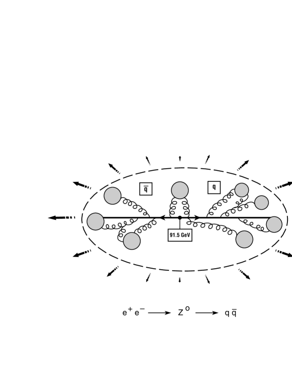
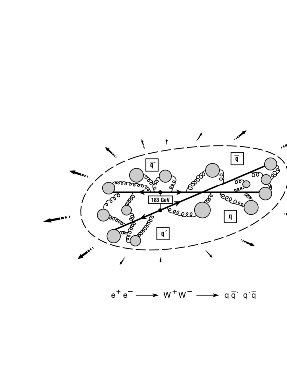
Figure 3: Schematics of the two $e^{+}e^{-}$ event types (42) and (43): The final-state hadron distribution in $Z^{0}$ events (left) is due to exclusively ‘endogamous’ hadronization of the partonic offspring from the $q\bar{q}$ dijet, whereas in $W^{+}W^{-}$ events (right) there is, in addition, the possibility of ‘exogamous’ hadron production involving a mating of partons from the two different $W^{+}\rightarrow q\bar{q}^{\prime}$ and $W^{-}\rightarrow q^{\prime}\bar{q}$ dijets.

These two processes are of interest for several reasons:

• Generally, $e^{+}e^{-}$ collisions at $\sqrt{(}s)\geq 90$ GeV provide the “cleanest” environment of all high-energy particle collisions for studying the physics of Bose-Einstein correlations, because there is no background to the interesting particles emitted from the calculable parton shower, and final-state hadrons escape unscathed from their emission point without further interactions. Correlation measurements can therefore be very valuable, as they may be used to calibrate analogous analyses in the extreme opposite case of heavy-ion collisions, where the emission region is more difficult to calculate accurately, and final-state hadron scattering and cascading can crucially influence the shape of the particle distributions.

• The experimental study of $e^{+}e^{-}\rightarrow Z^{0}\rightarrow hadrons$ at LEP 1 is based on several million events, and hence is impressively extensive and accurate. In particular, high-precision measurements of two- and three-particle correlations have been reported [14]. On the other hand, the reaction $e^{+}e^{-}\rightarrow W^{+}W^{-}\rightarrow hadrons$ is currently under very active study at LEP 2, in both its experimental and theoretical aspects: for an overview, see [48]. The interest in this reaction stems from its importance for measuring the triple-gauge-boson couplings and $m_{W}$. In particular, it has been argued that Bose-Einstein correlations may introduce an important source of systematic error into the analysis of $m_{W}$.

Theoretical studies of Bose-Einstein enhancements have mainly been within the context of the string models [1], which have been very successful in explaining the distributions of identical particles seen in high-energy $e^{+}e^{-}$ collisions [11]. Although the string description [1] of the hadronization process is a very appealing phenomenological approach and also has many other successes, it is not the only possible description. We employ a rather distinct cluster hadronization model, based on a space-time description of the perturbative development of parton showers, combined with a non-perturbative model for cluster formation and hadronization [2].

The crucial physics point is that, whatever model one uses for the details of the conversion of colored partons into color-neutral hadronic states, the Bose-Einstein correlations measured in $e^{+}e^{-}$ experiments are sensitive to local volumes of the order of a fermi in both the longitudinal and transverse directions. Therefore they provide important information on the intimate space-time structure of the hadronization mechanism. In particular, the sources that emit the final-state pions and other particles must be identified with local hadronization ‘patches’, and not with the system as a whole, which may extend over even hundreds of fermi. In the string picture, these local patches are the centers of string fragments, whereas in our cluster description the patches are elementary color-neutral clusters formed from the mating of nearest-neighbor partons. The effective Bose-Einstein correlation length should correpond to the sizes of these patches, namely the typical string extension $\simeq 1$ fm or the mean cluster size $\simeq 0.8$ fm. Loosely speaking, this correlation length defines the minimum possible distance that one may resolve from the particle distributions of the hadronic final state. Before turning to our model-specific analysis of the Bose-Einstein effect in $e^{+}e^{-}$ collisions, we refer the interested reader to the comprehensive overview [49], in which the status of related experimental and theoretical research in $e^{+}e^{-}$ physics can be found.

4.1 Modelling the space-time development of $e^{+}e^{-}$ collisions

In order to analyze the effects of identical-particle correlations in $e^{+}e^{-}$ collisions using the quantum version of the Bose-Einstein afterburner, we need to concentrate on event generators that deliver realistic, though classical, phase-space distributions of final-state hadrons, to which we may then apply the afterburner simulation of quantum interference and the Bose-Einstein effect. It is clear from the preceding Sections that such an event generator must not only give the momentum spectra, but also the vital space-time information on the dynamical evolution and in particular on the final stage of hadron emission. Unfortunately, most of the advanced event generators in particle physics [50] do not encode the relevant particle emission structure in space and time, whereas most event genarators for heavy-ion collisions do, but cannot be applied to $e^{+}e^{-}$ physics. One event generator that does satisfy both these requirements is VNI [18], which simulates the $e^{+}e^{-}$ collision dynamics all the way from the hard annihilation vertex, through the perturbative QCD shower development to the emergence of hadronic final states. Within the framework of relativistic quantum kinetics [51], the event generation in VNI traces in both space-time and momentum space the parton-shower evolution from the initial quark-antiquark pairs, followed by the clustering of the emitted quark and gluon offspring to pre-hadronic cluster states that then decay into the final-state hadrons. Referring to [9, 18] for details, we recall briefly here the essential concepts of this space-time model:

(i)

The parton-shower dynamics is described by conventional perturbative QCD evolution Monte Carlo methods, with the added feature that we keep track of the spatial development in a series of small time increments. Our procedure implements perturbative QCD transport theory in a manner consistent with the appropriate quantum-mechanical uncertainty principle, incorporating parton branching due to real and virtual quantum corrections involving gluons or quark-antiquark pairs. In the rest frame of the $Z^{0}$ (for (42)) or of the $W^{\pm}$ (for (43)), each off-shell parton $i$ in the shower propagates for a time $\Delta t_{i}$ given in the mean by $<\Delta t_{i}>=\gamma_{i}\tau_{i}=E_{i}/k^{2}_{i}=x_{i}M/2k^{2}_{i}$, where $k^{2}_{i}$ is the parton’s squared-momentum virtuality, and $x_{i}=E_{i}/M$ is its longitudinal energy fraction, during which it travels a distance $\Delta r_{i}=\Delta t_{i}\beta_{i}$, where $M=M_{Z^{0}}$ for (42) and $M=M_{W}$ for (43). It has been shown [9] that such a description results in a typical inside-outside perturbative cascade [52].

(ii)

The parton-hadron conversion is handled using a strictly spatial criterion for confinement, with a simple Ansatz for the probability $P(r)$ that nearest-neighbor color charges coalesce to color-neutral clusters in accord with their color and flavor degrees of freedom, where $r$ is the relative distance in between them in their center-of-mass frame. The nearest-neighbor criterion is imposed at each time step in the shower development, in such a way that every parton that is further from its neighbors than a certain critical distance $R_{c}=0.8$ fm has a probability distribution smeared around $R_{c}$ for combining with its nearest-neighbour parton to form a pre-hadronic cluster, possibly accompanied by one or more partons to take correct account of the colour flow. It is important to stress that at no moment in this shower development do we incorporate any prejudice regarding the genealogical origin of the partons: an ‘exogamous’ [10] pair of partons from different mother $q{\bar{q}}^{\prime}$ pairs have the same probability of coalescing into a hadronic cluster as do an ‘endogamous’ pair of partons from the same mother, at the same spatial separation. The resulting hadronic clusters are then allowed to decay into stable hadrons according to the particle data tables.

In the present paper, due to the less demanding requirements on event statistics, we will use the “quantum” version of the Bose-Einstein afterburner. This requires fixing the wave packet width $\sigma$ in the algorithm. Lacking convincing arguments for a unique physical choice of this parameter, we try to connect it with the intrinsic size $R_{c}$ of the pre-hadronic clusters which act as pion-emitting sources. The size $R_{c}$ also defines the minimum distance of adjacent clusters at formation without overlapping. We thus set

$$R_{c}=0.8\;\mbox{fm}=\sigma\,.$$ (44)

Finally, we stress that, although the event generation of $e^{+}e^{-}$ collisions along the above lines should provide a rather realistic simulation of the particle dynamics, we do not claim our results to be more than qualitative at this point, mainly since we have not included final-state interactions among the produced hadrons due to either Coulomb or strong interactions. In our approximation, the production vertex of each final-state hadron marks the last point of interaction, beyond which the particles stream freely on classical trajectories. Since in ‘real-life’ experiments these final-state interactions can become large at small relative momenta, one should be careful when comparing to measured data, some of which have been corrected for final-state interactions, others not.

4.2 Results for two-pion correlations

4.2.1 Multiplicity distributions

Figure 4: Multiplicity distributions of single pions (top) and of pairs of identical pions (bottom), per charged pion species.

It is plausible that the structure of the hadronic final state in $e^{+}e^{-}\rightarrow W^{+}W^{-}\rightarrow q\bar{q}^{\prime}\,q^{\prime}\bar{q}$ may not merely be a copy of $W^{\pm}\rightarrow q\bar{q}^{\prime}$ with twice the final-state multiplicity. As discussed in detail in [10, 9], it was found within our space-time parton-shower model that not only the total multiplicity $N(W^{+}W^{-})$ may be smaller than $2\times N(W^{\pm})$, but also that the particle spectra may exhibit characteristic differences. These differences are due to the special geometry of $W^{+}W^{-}$ events, in which the partonic offspring of the $W^{+}$ dijet overlap in space-time with the partons emitted from the $W^{-}$ dijet. The cross-talk between the quanta from the $W^{\pm}$ is especially prominent at small rapidities and if the two dijets emerge at small relative angles. Then, whereas in $e^{+}e^{-}\rightarrow Z^{0}$ decays all particles come from the same mother and only ‘endogamous’ cluster formation is possible, as in the left part of Fig. 3, $W^{+}W^{-}$ events receive a significant contribution from the coalescence of partons from different $W^{\pm}$ mothers into ‘exogamous’ clusters, as in the right part of Fig. 3.

Fig. 4 reflects the effects of parton ‘exogamy’ in $e^{+}e^{-}\rightarrow W^{+}W^{-}\rightarrow q\bar{q}^{\prime}\,q^{\prime}\bar{q}$ as compared to $Z^{0}\rightarrow q\bar{q}$, in the multiplicity distributions of both single pions (top) and of pairs of identical pions (bottom). Even allowing for the slightly larger mass of the $Z^{0}$ compared to the $W^{\pm}$, one observes, in agreement with the above discussion, an effective reduction $N_{\pi^{\pm}}(W^{+}W^{-})<2\times N_{\pi^{\pm}}(Z^{0})$, namely, $\langle N_{\pi^{\pm}}(Z^{0})\rangle=6.1$ versus $\langle N_{\pi^{\pm}}(W^{+}W^{-})\rangle=9.5$, per pion species. Similarly, we find for the number of identical-pion pairs $N_{\pi^{\pm}\pi^{\pm}}=N_{\pi^{\pm}}(N_{\pi^{\pm}}-1)$ that $N_{\pi^{\pm}\pi^{\pm}}(W^{+}W^{-})<4\times N_{\pi^{\pm}\pi^{\pm}}(Z^{0})$, namely, $\langle N_{\pi^{\pm}\pi^{\pm}}(Z^{0})\rangle=81.9$ versus $\langle N_{\pi^{\pm}\pi^{\pm}}(W^{+}W^{-})\rangle=207.3$.

The effect may be thought of as reflecting increased ‘efficiency’ in the hadronization process, due to the fact that the presence of two cross-talking dijets in the $W^{+}W^{-}$ decays, with their spatially-overlapping offspring, allows the evolving particle system to reorganize itself more favorably in the cluster-hadronization process, and to form clusters with smaller invariant mass than in the $Z^{0}$ events. Indeed, it was found in [10] that the mass spectrum of pre-hadronic clusters from coalescing partons is in fact softer in the $W^{+}W^{-}$ case, reflecting the fact that the availability of more partons enables clusters to form from configurations with lower invariant mass than in the $Z^{0}$ case.

4.2.2 Origins of pions

In theory, all pairs of identical pions can exhibit Bose-Einstein correlations. Experimentally, however, the measurements of the pair spectrum in the relative pair momentum $q$ run out of statistics because the phase space vanishes at very low $q$. Since small $q$ values correspond to large spatial distances, this region of $q$ is particularly sensitive to the decays into pions of long-living resonances, and also to long-range Coulomb or strong final-state interactions among the particles. Whereas final-state interaction effects can be corrected, this is not easy for resonance decays. Since many of the pions in $e^{+}e^{-}$ collisions have their origins in the decays of other particles with lifetimes significantly greater than a few fermis, it is useful to disentangle the various experimental sources of pions (or other particles) and to classify their parents as follows [49, 53, 54]:

• Prompt production leading to pions that emerge directly from the hadronization of the fragmenting system, whose parents may be visualized as decaying strings or (in our case) as pre-hadronic clusters.

• Short-lived particles such as $\rho$, $K^{\ast}$ and $\Delta$, that are strongly-decaying particles with decay lengths shorter than a few fermis.

• Long-lived resonances, such as $\eta,\eta^{\prime},\omega,\phi$, that are states which also decay strongly but have life-times of many fermis.

• ‘Stable’ particles, such as $\Lambda$ and $K_{s}^{0}$, that are particles which propagate sufficiently far that the pions emerging can be removed by track cuts.

• Weakly-decaying particles, such as charm or bottom mesons.

origin	life-time $\tau$	fraction
clusters	$<$ 0.5 fm	0.31
$\rho,\Delta,K^{\ast}$	1.3 $-$ 4 fm	0.41
$\eta,\eta^{\prime},\omega,\phi$	$>$ 10 fm	0.28

Table 1: Relative contributions of different sources of pions in our $e^{+}e^{-}$ event simulations.

In Table 1, we list the fractions of pions coming from these different sources, as estimated in our model simulations. Since the ‘stable’ particles can be considered as not having decayed, and weakly-decaying particles contribute only a negligible fraction, we do not include these two categories in the list. We observe that the numbers in Table 1 are very similar to those reported in [49].

4.2.3 The pion correlator $C(q,K)$ for $K=0$

Fig. 5 shows the correlator $C({\leavevmode\mathchoice{\hbox{\rm tensysevensyfivesy\boldmath{$\displaystyle q$}}}{\hbox{\rm tensysevensyfivesy\boldmath{$\textstyle q$}}}{\hbox{\rm tensysevensyfivesy\boldmath{$\scriptstyle q$}}}{\hbox{\rm tensysevensyfivesy\boldmath{$\scriptscriptstyle q$}}}},{\leavevmode\mathchoice{\hbox{\rm tensysevensyfivesy\boldmath{$\displaystyle K$}}}{\hbox{\rm tensysevensyfivesy\boldmath{$\textstyle K$}}}{\hbox{\rm tensysevensyfivesy\boldmath{$\scriptstyle K$}}}{\hbox{\rm tensysevensyfivesy\boldmath{$\scriptscriptstyle K$}}}})-1$ for different tensysevensyfivesy$\textstyle q$-values and vanishing pair momentum tensysevensyfivesy$\textstyle K$ in the c.m. frame of the collision, $C(q_{z},q_{s},q_{o},\leavevmode\mathchoice{\hbox{\rm tensysevensyfivesy\boldmath{$\displaystyle 0$}}}{\hbox{\rm tensysevensyfivesy\boldmath{$\textstyle 0$}}}{\hbox{\rm tensysevensyfivesy\boldmath{$\scriptstyle 0$}}}{\hbox{\rm tensysevensyfivesy\boldmath{$\scriptscriptstyle 0$}}})-1$. Two interesting observations can be made immediately:

Figure 5: The correlation function of same-sign pions for different values of the relative pair momentum tensysevensyfivesy$\textstyle q$ for vanishing pair momentum tensysevensyfivesy$\textstyle K$, $C(q_{z},q_{s},q_{o},\leavevmode\mathchoice{\hbox{\rm tensysevensyfivesy\boldmath{$\displaystyle 0$}}}{\hbox{\rm tensysevensyfivesy\boldmath{$\textstyle 0$}}}{\hbox{\rm tensysevensyfivesy\boldmath{$\scriptstyle 0$}}}{\hbox{\rm tensysevensyfivesy\boldmath{$\scriptscriptstyle 0$}}})-1$.

a) In both cases, $e^{+}e^{-}\rightarrow Z^{0}\rightarrow q\bar{q}\rightarrow\pi^{\prime}s$ and $e^{+}e^{-}\rightarrow W^{+}W^{-}\rightarrow q\bar{q}^{\prime}\,q^{\prime}\bar{q}\rightarrow\pi^{\prime}s$, we see no significant differences between the three relative momentum directions $q_{z},q_{s},q_{o}$. Although, for a fixed direction $q_{i}$, the intercept of the correlator at $q_{i}=0$ depends on the magnitude of the momentum transverse to $q_{i}$, it looks the same for $q_{i}=q_{z}$, $q_{i}=q_{s}$ or $q_{i}=q_{o}$.

b) The correlation function in the case $e^{+}e^{-}\rightarrow W^{+}W^{-}\rightarrow q\bar{q}^{\prime}\,q^{\prime}\bar{q}\rightarrow\pi^{\prime}s$ is slightly narrower than that of $e^{+}e^{-}\rightarrow Z^{0}\rightarrow q\bar{q}\rightarrow\pi^{\prime}s$. Since the mean $q$ values correspond to the inverses of the typical emission source sizes, this means that the hadronic $W^{+}W^{-}$ decays reflect a larger source size ($\simeq 1$ fm) than the $Z^{0}$ decays ($\simeq 0.8$ fm), as we discuss later in the context of resonance effects.

The implication of observation a) is that the pion emission appears essentially spherically symmetric with respect to the three orthogonal directions $q_{z},q_{s},q_{o}$. This may appear to conflict with the naive expectation that the source should appear much more elongated in the longitudinal $z$ direction than in the sideward and outward $s,o$ directions, because of the large longitudinal momenta of the leading quark jets. However, as we pointed out before, in this model the pre-hadronic cluster formation is controlled by the ‘nearest-neighbor’ criterion, so that only spatially adjacent partons with a mean separation $R_{c}\sim 0.8$ fm have a significant probability of coalescing and decaying into pions and other hadrons. This local coalescence results naturally in a longitudinal-momentum ordering of particles as a function of their distance from the jet origin: particles further away tend to have higher momentum than those in the center. Since the Bose-Einstein effect is only apparent for identical particles with similar momenta, corresponding to small $q$, particles that are separated by many fermi at production are incapable of showing a significant enhancement because their momenta are so different.

One may conclude from observation b) that parton ‘exogamy’ in $W^{+}W^{-}$ decays [10] results in a space-time distribution of hadrons that is more spread out than in the case of $Z^{0}$ decays. This may again be understood as a consequence of increased efficiency of hadron formation in the $W^{+}W^{-}$ events, as we discussed before in the context of the pion multiplicity distributions in Fig. 4. The identical pions emerging as products of parton-cluster decays have a longer distance correlation in $W^{+}W^{-}$ events, because the partonic offspring of the overlapping $q\bar{q}$ dijets are enhanced mainly for low-momentum quanta in the central rapidity region, corresponding to significant ‘exogamous’ coalescence of partons from different $W$’s with small relative momenta. As a consequence, the pion pair spectrum from $W^{+}W^{-}$ decays in Fig. 5b is narrower than the one from $Z^{0}$ decays in Fig. 5a, which translates into a larger effective emission radius for these pions.

4.2.4 The pion correlator $C(q,K)$ for $K\neq 0$

The general features and physics interpretation of the tensysevensyfivesy$\textstyle K$-dependence of the correlation function $C({\leavevmode\mathchoice{\hbox{\rm tensysevensyfivesy\boldmath{$\displaystyle q$}}}{\hbox{\rm tensysevensyfivesy\boldmath{$\textstyle q$}}}{\hbox{\rm tensysevensyfivesy\boldmath{$\scriptstyle q$}}}{\hbox{\rm tensysevensyfivesy\boldmath{$\scriptscriptstyle q$}}}},{\leavevmode\mathchoice{\hbox{\rm tensysevensyfivesy\boldmath{$\displaystyle K$}}}{\hbox{\rm tensysevensyfivesy\boldmath{$\textstyle K$}}}{\hbox{\rm tensysevensyfivesy\boldmath{$\scriptstyle K$}}}{\hbox{\rm tensysevensyfivesy\boldmath{$\scriptscriptstyle K$}}}})$ have been studied in detail in [26, 28, 54]. A manifest change in the shape of $C({\leavevmode\mathchoice{\hbox{\rm tensysevensyfivesy\boldmath{$\displaystyle q$}}}{\hbox{\rm tensysevensyfivesy\boldmath{$\textstyle q$}}}{\hbox{\rm tensysevensyfivesy\boldmath{$\scriptstyle q$}}}{\hbox{\rm tensysevensyfivesy\boldmath{$\scriptscriptstyle q$}}}},{\leavevmode\mathchoice{\hbox{\rm tensysevensyfivesy\boldmath{$\displaystyle K$}}}{\hbox{\rm tensysevensyfivesy\boldmath{$\textstyle K$}}}{\hbox{\rm tensysevensyfivesy\boldmath{$\scriptstyle K$}}}{\hbox{\rm tensysevensyfivesy\boldmath{$\scriptscriptstyle K$}}}})$ as tensysevensyfivesy$\textstyle K$ varies can have several origins, the two most important being (i) resonance decay contributions [54, 55] and (ii) collective flow of the particle matter [26]. Whereas pions from long-lived resonances are always present in high-energy collisions, collective motion of the produced particles is a feature of heavy-ion reactions that produce high-density matter, but certainly is not an issue for the $e^{+}e^{-}$ collisions discussed here. In this subsection we do not distinguish the contributions from resonance decays, but show the tensysevensyfivesy$\textstyle K$-dependence of the correlation function including pions from long-lived resonances, just as in the previous figures. We disentangle the effect of resonance decays in the next subsection.

Fig. 6 shows the correlation function $C({\leavevmode\mathchoice{\hbox{\rm tensysevensyfivesy\boldmath{$\displaystyle q$}}}{\hbox{\rm tensysevensyfivesy\boldmath{$\textstyle q$}}}{\hbox{\rm tensysevensyfivesy\boldmath{$\scriptstyle q$}}}{\hbox{\rm tensysevensyfivesy\boldmath{$\scriptscriptstyle q$}}}},{\leavevmode\mathchoice{\hbox{\rm tensysevensyfivesy\boldmath{$\displaystyle K$}}}{\hbox{\rm tensysevensyfivesy\boldmath{$\textstyle K$}}}{\hbox{\rm tensysevensyfivesy\boldmath{$\scriptstyle K$}}}{\hbox{\rm tensysevensyfivesy\boldmath{$\scriptscriptstyle K$}}}})-1$ of same-sign pions for various values of the pair momentum ${\leavevmode\mathchoice{\hbox{\rm tensysevensyfivesy\boldmath{$\displaystyle K$}}}{\hbox{\rm tensysevensyfivesy\boldmath{$\textstyle K$}}}{\hbox{\rm tensysevensyfivesy\boldmath{$\scriptstyle K$}}}{\hbox{\rm tensysevensyfivesy\boldmath{$\scriptscriptstyle K$}}}}=(K_{L},{\leavevmode\mathchoice{\hbox{\rm tensysevensyfivesy\boldmath{$\displaystyle K$}}}{\hbox{\rm tensysevensyfivesy\boldmath{$\textstyle K$}}}{\hbox{\rm tensysevensyfivesy\boldmath{$\scriptstyle K$}}}{\hbox{\rm tensysevensyfivesy\boldmath{$\scriptscriptstyle K$}}}}_{\perp})$, where $K_{L}=K_{z}$ is the direction along the thrust axis and $K_{\perp}=|{\leavevmode\mathchoice{\hbox{\rm tensysevensyfivesy\boldmath{$\displaystyle K$}}}{\hbox{\rm tensysevensyfivesy\boldmath{$\textstyle K$}}}{\hbox{\rm tensysevensyfivesy\boldmath{$\scriptstyle K$}}}{\hbox{\rm tensysevensyfivesy\boldmath{$\scriptscriptstyle K$}}}}_{\perp}|=\sqrt{K_{x}^{2}+K_{y}^{2}}$ the momentum transverse to it. The correlator is plotted as a function of one of the three Cartesian components of the relative momentum tensysevensyfivesy$\textstyle q$, with the other two components set to zero. The two main features are:

Figure 6: The correlation function of same-sign pions $C({\leavevmode\mathchoice{\hbox{\rm tensysevensyfivesy\boldmath{$\displaystyle q$}}}{\hbox{\rm tensysevensyfivesy\boldmath{$\textstyle q$}}}{\hbox{\rm tensysevensyfivesy\boldmath{$\scriptstyle q$}}}{\hbox{\rm tensysevensyfivesy\boldmath{$\scriptscriptstyle q$}}}},{\leavevmode\mathchoice{\hbox{\rm tensysevensyfivesy\boldmath{$\displaystyle K$}}}{\hbox{\rm tensysevensyfivesy\boldmath{$\textstyle K$}}}{\hbox{\rm tensysevensyfivesy\boldmath{$\scriptstyle K$}}}{\hbox{\rm tensysevensyfivesy\boldmath{$\scriptscriptstyle K$}}}})-1$ for various values of the pair momentum ${\leavevmode\mathchoice{\hbox{\rm tensysevensyfivesy\boldmath{$\displaystyle K$}}}{\hbox{\rm tensysevensyfivesy\boldmath{$\textstyle K$}}}{\hbox{\rm tensysevensyfivesy\boldmath{$\scriptstyle K$}}}{\hbox{\rm tensysevensyfivesy\boldmath{$\scriptscriptstyle K$}}}}=(K_{L},{\leavevmode\mathchoice{\hbox{\rm tensysevensyfivesy\boldmath{$\displaystyle K$}}}{\hbox{\rm tensysevensyfivesy\boldmath{$\textstyle K$}}}{\hbox{\rm tensysevensyfivesy\boldmath{$\scriptstyle K$}}}{\hbox{\rm tensysevensyfivesy\boldmath{$\scriptscriptstyle K$}}}}_{\perp})$, where $K_{L}=K_{z}$ is the direction along the thrust axis and $K_{\perp}=|{\leavevmode\mathchoice{\hbox{\rm tensysevensyfivesy\boldmath{$\displaystyle K$}}}{\hbox{\rm tensysevensyfivesy\boldmath{$\textstyle K$}}}{\hbox{\rm tensysevensyfivesy\boldmath{$\scriptstyle K$}}}{\hbox{\rm tensysevensyfivesy\boldmath{$\scriptscriptstyle K$}}}}_{\perp}|=\sqrt{K_{x}^{2}+K_{y}^{2}}$ is the momentum transverse to it. The correlators are plotted against one component of the relative momentum, setting the two other components to zero.

a) The shape of the correlation function flattens and widens as $K_{L}$ or $K_{\perp}$ are increased. However, the mean $q_{L,\perp}$ change by less than 10 % when the $K_{L,T}$ values are varied from 0 to 1 GeV.

b) The tensysevensyfivesy$\textstyle K$-dependence is evidently spherically symmetric, i.e., the correlation function changes in the same way as $K_{L}$ or $K_{\perp}$ is increased in the range from 0 to 1 GeV.

Point a) is a reflection of resonance-decay pions: long-lived resonances with $\tau>10$ fm can travel for many fermis before decaying, which leads to an exponential tail in the pion pair spectrum [54]. This ‘life-time effect’ is larger for small values of tensysevensyfivesy$\textstyle K$ and damps out as tensysevensyfivesy$\textstyle K$ is increased, since the relative abundance of resonances is most pronounced at small tensysevensyfivesy$\textstyle K$.

Point b), on the other hand, is in accord with the fact that the kinematics is approximately boost-invariant along the thrust axis of the $e^{+}e^{-}$ collision, and the ‘local’ character of the particle dynamics in our model. Neither the parton shower evolution nor the parton-cluster hadronization depend on the overall momentum tensysevensyfivesy$\textstyle K$ relative to the $e^{+}e^{-}$ center-of-mass frame, as it is only the kinematics, color and flavor of the near-by clustering partons which at any given vertex determines locally the development of particle production.

4.2.5 Effects of resonance decays on $C(q,K)$

Consider now a pair of identical pions with relative momentum tensysevensyfivesy$\textstyle q$, where one of the pions originates from a resonance of momentum tensysevensyfivesy$\textstyle p$ with mass $m_{r}$ and decay width $\Gamma_{r}\sim\tau_{r}^{-1}$. Such a pair cannot contribute to the Bose-Einstein effect if $|{\leavevmode\mathchoice{\hbox{\rm tensysevensyfivesy\boldmath{$\displaystyle q$}}}{\hbox{\rm tensysevensyfivesy\boldmath{$\textstyle q$}}}{\hbox{\rm tensysevensyfivesy\boldmath{$\scriptstyle q$}}}{\hbox{\rm tensysevensyfivesy\boldmath{$\scriptscriptstyle q$}}}}\cdot\leavevmode\mathchoice{\hbox{\rm tensysevensyfivesy\boldmath{$\displaystyle p$}}}{\hbox{\rm tensysevensyfivesy\boldmath{$\textstyle p$}}}{\hbox{\rm tensysevensyfivesy\boldmath{$\scriptstyle p$}}}{\hbox{\rm tensysevensyfivesy\boldmath{$\scriptscriptstyle p$}}}|\gg m_{r}\Gamma_{r}$, which roughly implies that $|{\leavevmode\mathchoice{\hbox{\rm tensysevensyfivesy\boldmath{$\displaystyle q$}}}{\hbox{\rm tensysevensyfivesy\boldmath{$\textstyle q$}}}{\hbox{\rm tensysevensyfivesy\boldmath{$\scriptstyle q$}}}{\hbox{\rm tensysevensyfivesy\boldmath{$\scriptscriptstyle q$}}}}|\gg\tau_{r}^{-1}$. Since tensysevensyfivesy$\textstyle q$ is inversely proportional to the spatial dimension of the pion source, this means that resonances represent a source of spatial extent of the order of $\tau_{r}^{-1}$. Hence, such pions only can exhibit correlations if $|{\leavevmode\mathchoice{\hbox{\rm tensysevensyfivesy\boldmath{$\displaystyle q$}}}{\hbox{\rm tensysevensyfivesy\boldmath{$\textstyle q$}}}{\hbox{\rm tensysevensyfivesy\boldmath{$\scriptstyle q$}}}{\hbox{\rm tensysevensyfivesy\boldmath{$\scriptscriptstyle q$}}}}|\leq O(\tau_{r}^{-1})$, which for long-living resonances ($\tau_{r}\geq 10$ fm) requires $|{\leavevmode\mathchoice{\hbox{\rm tensysevensyfivesy\boldmath{$\displaystyle q$}}}{\hbox{\rm tensysevensyfivesy\boldmath{$\textstyle q$}}}{\hbox{\rm tensysevensyfivesy\boldmath{$\scriptstyle q$}}}{\hbox{\rm tensysevensyfivesy\boldmath{$\scriptscriptstyle q$}}}}|\leq 20$ MeV. This is less than the scale at which direct pions coming from the pre-hadronic clusters contribute, as seen in Table 1. Therefore the pion correlation function $C({\leavevmode\mathchoice{\hbox{\rm tensysevensyfivesy\boldmath{$\displaystyle q$}}}{\hbox{\rm tensysevensyfivesy\boldmath{$\textstyle q$}}}{\hbox{\rm tensysevensyfivesy\boldmath{$\scriptstyle q$}}}{\hbox{\rm tensysevensyfivesy\boldmath{$\scriptscriptstyle q$}}}},{\leavevmode\mathchoice{\hbox{\rm tensysevensyfivesy\boldmath{$\displaystyle K$}}}{\hbox{\rm tensysevensyfivesy\boldmath{$\textstyle K$}}}{\hbox{\rm tensysevensyfivesy\boldmath{$\scriptstyle K$}}}{\hbox{\rm tensysevensyfivesy\boldmath{$\scriptscriptstyle K$}}}})$ is narrowed by the effects of the pion decay products of long-living resonances.

Figure 7: The correlator $C({\leavevmode\mathchoice{\hbox{\rm tensysevensyfivesy\boldmath{$\displaystyle q$}}}{\hbox{\rm tensysevensyfivesy\boldmath{$\textstyle q$}}}{\hbox{\rm tensysevensyfivesy\boldmath{$\scriptstyle q$}}}{\hbox{\rm tensysevensyfivesy\boldmath{$\scriptscriptstyle q$}}}},{\leavevmode\mathchoice{\hbox{\rm tensysevensyfivesy\boldmath{$\displaystyle K$}}}{\hbox{\rm tensysevensyfivesy\boldmath{$\textstyle K$}}}{\hbox{\rm tensysevensyfivesy\boldmath{$\scriptstyle K$}}}{\hbox{\rm tensysevensyfivesy\boldmath{$\scriptscriptstyle K$}}}})-1$ for ${\leavevmode\mathchoice{\hbox{\rm tensysevensyfivesy\boldmath{$\displaystyle K$}}}{\hbox{\rm tensysevensyfivesy\boldmath{$\textstyle K$}}}{\hbox{\rm tensysevensyfivesy\boldmath{$\scriptstyle K$}}}{\hbox{\rm tensysevensyfivesy\boldmath{$\scriptscriptstyle K$}}}}=\leavevmode\mathchoice{\hbox{\rm tensysevensyfivesy\boldmath{$\displaystyle 0$}}}{\hbox{\rm tensysevensyfivesy\boldmath{$\textstyle 0$}}}{\hbox{\rm tensysevensyfivesy\boldmath{$\scriptstyle 0$}}}{\hbox{\rm tensysevensyfivesy\boldmath{$\scriptscriptstyle 0$}}}$ with (solid curves) and without (dashed lines) the contributions from long-lived resonances.

To quantify the resonance narrowing and localize the pile-up of pion pairs where at least one comes from resonance decay, we have disentangled the pion emission sources of Table 1 within our event simulation. In Fig. 7 we show again the correlator $C({\leavevmode\mathchoice{\hbox{\rm tensysevensyfivesy\boldmath{$\displaystyle q$}}}{\hbox{\rm tensysevensyfivesy\boldmath{$\textstyle q$}}}{\hbox{\rm tensysevensyfivesy\boldmath{$\scriptstyle q$}}}{\hbox{\rm tensysevensyfivesy\boldmath{$\scriptscriptstyle q$}}}},{\leavevmode\mathchoice{\hbox{\rm tensysevensyfivesy\boldmath{$\displaystyle K$}}}{\hbox{\rm tensysevensyfivesy\boldmath{$\textstyle K$}}}{\hbox{\rm tensysevensyfivesy\boldmath{$\scriptstyle K$}}}{\hbox{\rm tensysevensyfivesy\boldmath{$\scriptscriptstyle K$}}}})-1$ for ${\leavevmode\mathchoice{\hbox{\rm tensysevensyfivesy\boldmath{$\displaystyle K$}}}{\hbox{\rm tensysevensyfivesy\boldmath{$\textstyle K$}}}{\hbox{\rm tensysevensyfivesy\boldmath{$\scriptstyle K$}}}{\hbox{\rm tensysevensyfivesy\boldmath{$\scriptscriptstyle K$}}}}=\leavevmode\mathchoice{\hbox{\rm tensysevensyfivesy\boldmath{$\displaystyle 0$}}}{\hbox{\rm tensysevensyfivesy\boldmath{$\textstyle 0$}}}{\hbox{\rm tensysevensyfivesy\boldmath{$\scriptstyle 0$}}}{\hbox{\rm tensysevensyfivesy\boldmath{$\scriptscriptstyle 0$}}}$ in the two cases of $e^{+}e^{-}\rightarrow W^{+}W^{-}\rightarrow q\bar{q}^{\prime}\,q^{\prime}\bar{q}\rightarrow\pi$’s and $e^{+}e^{-}\rightarrow Z^{0}\rightarrow q\bar{q}\rightarrow\pi$’s. The full lines correspond to the correlator with all sources included, as in the previous Fig. 6, whereas the dashed curves have the long-living resonance decay contributions removed. One sees that the resonance decay pions make a significant 20 - 30 % contribution to the magnitude of $C-1$ at $q_{L},q_{T}\,\lower 3.0pt\hbox{$\buildrel<\over{\sim}$}\,50$ MeV, corresponding to life-times $>5$ fm.

Figure 8: The tensysevensyfivesy$\textstyle K$ dependence of the effective pion source radii associated with the mean values of the components of ${\leavevmode\mathchoice{\hbox{\rm tensysevensyfivesy\boldmath{$\displaystyle q$}}}{\hbox{\rm tensysevensyfivesy\boldmath{$\textstyle q$}}}{\hbox{\rm tensysevensyfivesy\boldmath{$\scriptstyle q$}}}{\hbox{\rm tensysevensyfivesy\boldmath{$\scriptscriptstyle q$}}}}=(q_{L},q_{s},q_{o})$ in the longitudinal ($R_{L}$) and transverse ($R_{o},R_{s}$) directions with respect to the thrust axis. The solid lines include all sources, whereas the dashed curves exclude long-lived resonances.

Fig. 8 exhibits the tensysevensyfivesy$\textstyle K$-dependence of the effective emission radii associated with the mean values of the components of ${\leavevmode\mathchoice{\hbox{\rm tensysevensyfivesy\boldmath{$\displaystyle q$}}}{\hbox{\rm tensysevensyfivesy\boldmath{$\textstyle q$}}}{\hbox{\rm tensysevensyfivesy\boldmath{$\scriptstyle q$}}}{\hbox{\rm tensysevensyfivesy\boldmath{$\scriptscriptstyle q$}}}}=(q_{L},q_{s},q_{o})$ in the longitudinal ($R_{L}$) and transverse ($R_{o},R_{s}$) directions with respect to the thrust axis [54]:

$$R^{2}_{i}({\leavevmode\mathchoice{\hbox{\rm tensysevensyfivesy\boldmath{$\displaystyle K$}}}{\hbox{\rm tensysevensyfivesy\boldmath{$\textstyle K$}}}{\hbox{\rm tensysevensyfivesy\boldmath{$\scriptstyle K$}}}{\hbox{\rm tensysevensyfivesy\boldmath{$\scriptscriptstyle K$}}}})\;=\;\frac{1}{2\langle q_{i}^{2}\rangle}\;,\;\;\;\;\;\;\;\;\;\;\;\;\;\;\langle q_{i}^{2}\rangle\;=\;\frac{\int dq_{i}\,q_{i}^{2}\,\left[\,C(q_{i},{\leavevmode\mathchoice{\hbox{\rm tensysevensyfivesy\boldmath{$\displaystyle K$}}}{\hbox{\rm tensysevensyfivesy\boldmath{$\textstyle K$}}}{\hbox{\rm tensysevensyfivesy\boldmath{$\scriptstyle K$}}}{\hbox{\rm tensysevensyfivesy\boldmath{$\scriptscriptstyle K$}}}})-1\right]}{\int dq_{i}\,\left[\,C(q_{i},{\leavevmode\mathchoice{\hbox{\rm tensysevensyfivesy\boldmath{$\displaystyle K$}}}{\hbox{\rm tensysevensyfivesy\boldmath{$\textstyle K$}}}{\hbox{\rm tensysevensyfivesy\boldmath{$\scriptstyle K$}}}{\hbox{\rm tensysevensyfivesy\boldmath{$\scriptscriptstyle K$}}}})-1\right]}\;.$$ (45)

Again, the full lines include all the sources in Table 1, whereas the dashed lines exclude the long-living resonances. It is evident that the effect of resonances is most pronounced for small values of tensysevensyfivesy$\textstyle K$ and disappears with increasing tensysevensyfivesy$\textstyle K$. This is expected as the abundance of pions from resonance decays is most prominent at small tensysevensyfivesy$\textstyle K$. Resonance decays thus induce a pair-momentum dependence of the HBT radii [54, 55], with overall variations of the radii on the order of 0.1 fm.

It is interesting to note that after switching off the resonance decay contributions the HBT radii shown in Fig. 8 exhibit no remaining pair-momentum dependence. Such a pair-momentum dependence would signal the presence of position-momentum correlations in the source as, e.g., induced by collective flow or string breaking kinematics. No such correlations are visible here, not even along the thrust axis (see the left panels of Fig. 8 which show $R_{L}$ as a function of $K_{\perp}$). This is surprising because the inside-outside cascade features of parton and hadron production in VNI should lead to appreciable position-momentum correlations along the longitudinal axis defined by the primary hard partons. We can think of two possible reasons for the fact that they are not reflected in the longitudinal HBT radii shown here: either they get largely averaged out by summing over many collision events (which we think is unlikely), or they get covered up by the finite size of the wave packet width $\sigma$ in the Bose-Einstein afterburner. The fact that all HBT radii come out very close to $\sigma=0.8$ fm lends support to the second conjecture, although a final clarification of this issue has to await a comparison with calculations based on the “classical” version of the afterburner, as well as studies of the “quantum” version with different values of $\sigma$.

5 Discussion

We have discussed in this paper two possible algorithms for modelling Bose-Einstein correlations in a Monte Carlo code for $e^{+}e^{-}$ annihilation into hadrons, that incorporates information from perturbative QCD on the space-time evolution of parton showers and a configuration-space criterion for hadronization. Afterburners incorporating both the “classical” and “quantum” algorithms have been applied to a model in which the hadron emission region is known analytically. Standard tools for analyzing the sizes of hadron emission regions have been applied to these model calculations, and shown to reproduce successfully the parameters of the model. The quantum algorithm has then been implemented as an afterburner in the space-time parton-shower Monte Carlo, and applied to $e^{+}e^{-}\rightarrow Z^{0}\rightarrow hadrons$ and $e^{+}e^{-}\rightarrow W^{+}W^{-}\rightarrow hadrons$. Exploratory analyses have been presented of two-pion correlations in longitudinal and transverse momenta, both with and without resonance decays. The latter have been shown to modify significantly the Gaussian behaviour that would otherwise have been expected, and to cause a pair-momentum dependence of the extracted HBT radii, albeit on a small scale of order 0.1 fm only. In the limit studied here where the “quantum” afterburner was used with a fixed wave packet width $\sigma=0.8$ fm, resonance decays in fact induced the only discernible $K_{\perp}$-dependence of the HBT radii.

The analysis of this paper has necessarily been incomplete, and we conclude by listing some of the open questions that could be addressed in any future work. It would be interesting to implement the “classical” algorithm as an afterburner, and investigate the similarities and differences with the quantum afterburner explored in this paper. We are not in a position to express a definitive theoretical preference for one algorithm over the other. Within the context of the quantum afterburner, we have assumed one particular value of the Gaussian wave-packet size $\sigma$, and have not explored the implications of varying this parameter. In this connection, we should draw the reader’s attention to the possibility that the similarities between the correlations in the transverse and longitudinal momenta may be related to the choice of $\sigma$, which we have not attempted to optimize. This would involve an overall tuning of the Monte Carlo to fit particle spectra, which we are currently not in a position to complete. Once this is done, one could use the Monte Carlo to address some of the physics issues that triggered this investigation, including the possible effects of Bose-Einstein correlations on measurements of the $W^{\pm}$ mass in hadronic final states at LEP 2.

Despite the inevitable incompleteness of this work, we hope that the ideas and investigations reported here may be useful in future studies along the lines suggested above, either within the context of the space-time approach to $e^{+}e^{-}$ annihilation into hadrons used here, or within some other approach. The Bose-Einstein afterburners studied here could also be implemented in Monte Carlo codes for other interactions, including relativistic heavy-ion collisions. We are currently studying how this work could be advanced along these lines.

The authors acknowledge illuminating discussions with M. Gyulassy, J. Sollfrank, S. Vance and W.A. Zajc. We thank C. Slotta for assisting us with the figures. This work was supported in part by the Director, Office of Energy Research, Division of Nuclear Physics of the Office of High Energy and Nuclear Physics of the U.S. Department of Energy under Contract No. DE-FG02-93ER40764 and DE-AC02-76H00016.

References

• [1] B. Andersson, G. Gustafson, G. Ingelman, and T. Sjöstrand, Phys. Rep. 97, 33 (1983); B. Andersson, G. Gustafson and B. Söderberg, Nucl. Phys. B264, 29 (1986).
• [2] T. D. Gottschalk, Nucl. Phys. B214, 201 (1983) and Nucl. Phys. B227, 413 (1983); B. R. Webber, Nucl. Phys. B238, 492 (1984).
• [3] D. Amati and G. Veneziano, Phys. Lett. 83B, 87 (1979); D. Amati, A. Bassetto, M. Ciafaloni, G. Marchesini, and G. Veneziano, Nucl. Phys. B173, 429 (1980).
• [4] J. Ellis and K. Geiger, Phys. Rev. D 52, 1500 (1995); Nucl. Phys. A590, 609 (1995).
• [5] G. Gustafson, U. Pettersson, and P. Zerwas, Phys. Lett. B 209, 90 (1988).
• [6] T. Sjöstrand and V. A. Khoze, Phys. Rev. Lett. 72, 28 (1994); Z. Phys. C 62, 281 (1994).
• [7] G. Gustafson and J. Häkkinen, Z. Phys. C 64, 659 (1994).
• [8] L. Lönnblad, Z. Phys. C 70, 625 (1996).
• [9] J. Ellis and K. Geiger, Phys. Rev. D 54, 1967 (1996).
• [10] J. Ellis and K. Geiger, Phys. Lett. B 404, 230 (1997).
• [11] M. G. Bowler, Z. Phys. C 29, 617 (1985); B. Andersson and W. Hoffmann, Phys. Lett. B 169, 364 (1986); B. Andersson and M. Ringner, Phys. Lett. B 421, 283 (1998); J. Häkkinen M. Ringner, Eur. Phys. J. C5, 275 (1998).
• [12] L. Lönnblad and T. Sjöstrand, Phys. Lett. B 351, 293 (1995).
• [13] L. Lönnblad and T. Sjöstrand, Eur. Phys. J. C2, 165 (1998).
• [14] TPC Collaboration, Phys. Rev. D 31, 996 (1985); TASSO Collaboration, Z. Phys. C 30, 355 (1986); MARK II Collaboration, Phys. Rev. D 39, 39 (1989).
• [15] For analyses at the $Z^{0}$ peak, see:
ALEPH Collaboration, Z. Phys. C 54, 75 (1992); DELPHI Collaboration, Phys. Lett. B 268, 201 (1992); OPAL Collaboration, Eur. Phys. J. C5, 239 (1998) and references therein.
• [16] For recent analyses in $W^{+}W^{-}$ final states, see:
ALEPH Collaboration, paper 894; DELPHI Collaboration, paper 288; L3 Collaboration, paper 506; OPAL Collaboration, paper 391 contributed to the International Conference on High-Energy Physics, Vancouver, 1998.
• [17] Z. Kunszt et al., Proceedings of the Workshop on Physics at LEP2, CERN Yellow Report 96-01, eds. G. Altarelli, T. Sjöstrand and F. Zwirner, Vol. 1, 141 (1996).
• [18] K. Geiger, Comp. Phys. Com. 104, 70 (1997). The latest version of the computer program VNI can be obtained from http://rhic.phys.columbia.edu/rhic/vni.
• [19] K. Geiger, Phys. Rev. D 54, 949 (1996).
• [20] B.A. Campbell, J. Ellis and K.A. Olive, Phys. Lett. B 235, 325 (1990); and Nucl. Phys. B345, 57 (1990).
• [21] J. Ellis, K. Geiger and H. Kowalski, Phys. Rev. D 54, 5443 (1996).
• [22] K. Geiger and R. Longacre, Heavy Ion Phys. 8, 41 (1998).
• [23] K. Geiger and B. Müller, Heavy Ion Phys. 7, 207 (1998); K. Geiger, Phys. Rev. D 57, 1895 (1998).
• [24] K. Geiger and D.K. Srivastava, Phys. Lett. B 422, 39 (1998); nucl-th/9806050; nucl-th/9808042.
• [25] K. Fialkowski and R. Wit, Eur. Phys. J. C2, 691 (1998); hep-ph/9805476; hep-ph/9810492; K. Fialkowski, R. Wit and J. Wosiek, Phys. Rev. D 58, 094013 (1998); A. Bialas and K. Zalewski, hep-ph/9806435; S.V. Chekanov, E.A. De Wolf and W. Kittel, hep-ph/9809530.
• [26] U. Heinz, Nucl. Phys. A610, 264c (1996).
• [27] U.A. Wiedemann, B. Tomášik, and U. Heinz, Nucl. Phys. A638, 475c (1998).
• [28] U. Heinz, in Correlations and Clustering Phenomena in Subatomic Physics, eds. M.N. Harakeh, O. Scholten, and J.H. Koch, NATO ASI Series B 359, 137 (1997) (Plenum, New York); nucl-th/9710065; hep-ph/9806512.
• [29] Q.H. Zhang, U.A. Wiedemann, C. Slotta and U. Heinz, Phys. Lett. B 407, 33 (1997).
• [30] U.A. Wiedemann, P. Foka, H. Kalechofsky, M. Martin, C. Slotta and Q.H. Zhang, Phys. Rev. C 56, R614 (1997).
• [31] M. Martin, H. Kalechofsky, P. Foka and U.A. Wiedemann, Eur. Phys. J. C2 (1998) 359.
• [32] U.A. Wiedemann, J. Ellis, U. Heinz, and K. Geiger, to appear in CRIS’98: Measuring the size of things in the Universe: HBT interferometry and heavy ion physics, Catania, June 8-12, 1998, eds. S. Costa et al., (World Scientific, Singapore, 1998), nucl-th/9808043.
• [33] W.A. Zajc, in Particle Production in Highly Excited Matter, eds. H.H. Gutbrod and J. Rafelski, NATO ASI Series B 303, 435 (1993) (Plenum, New York).
• [34] B. Andersson and M. Ringner, Nucl. Phys. B513, 627 (1998); Phys. Lett. B 421, 283 (1998).
• [35] D.V. Anchishkin, U. Heinz, and P. Renk, Phys. Rev. C 57, 1428 (1998).
• [36] U.A. Wiedemann, Phys. Rev. C 57, 3324 (1998).
• [37] E. Shuryak, Phys. Lett. 44B, 387 (1973); Sov. J. Nucl. Phys. 18, 667 (1974).
• [38] S. Pratt, Phys. Rev. Lett. 53, 1219 (1984); Phys. Rev. D 33, 72 (1986).
• [39] S. Chapman and U. Heinz, Phys. Lett. B 340, 250 (1994).
• [40] M. Gyulassy, S.K. Kauffmann, and L.W. Wilson, Phys. Rev. C 20, 2267 (1979).
• [41] D. Miśkowiec and S. Voloshin, nucl-ex/9704006.
• [42] Q.H. Zhang, P. Scotto, and U. Heinz, nucl-th/9805046, to be published in Phys. Rev. C 58 (1st Dec., 1998).
• [43] G. Bertsch, Phys. Rev. Lett. 72, 2349 (1994).
• [44] S. Pratt, in Quark-Gluon Plasma 2, ed. R.C. Hwa (World Scientific, Singapore, 1995), p. 700.
• [45] S. Padula, M. Gyulassy, and S. Gavin, Nucl. Phys. B329, 357 (1990).
• [46] T. Csörgő and J. Zimányi, Phys. Rev. Lett. 80, 916 (1998); J. Zimányi and T. Csörgő, hep-ph/9705432.
• [47] T. Hebbeker, Phys. Rep. 217, 69 (1992); S. Bethke and J. E. Pilcher, Ann. Rev. Nucl. Part. Sci. 42, 251 (1992).
• [48] A. Ballestrero et al., J. Phys. G 24, 365 (1998).
• [49] S. Haywood, Rutherford-Appleton preprint RAL-94-074, (1994).
• [50] For example: G. Marchesini, B. R. Webber, G. Abbiendi, I. G. Knowles, M. H. Seymor anp L. Stanco, Comp. Phys. Com. 67, 465 (1992); L. Lönnblad, Comp. Phys. Com. 71, 15 (1992); T. Sjöstrand, Comp. Phys. Com. 82, 74 (1994).
• [51] K. Geiger, Phys. Rev. D 56, 2665 (1997).
• [52] G. Marchesini, L. Trentadue and G. Veneziano, Nucl. Phys. B181, 335 (1981); K. Konishi, CERN-TH.2853 (1980).
• [53] P. Grassberger, Nucl. Phys. B120, 231 (1977); M. Bowler, Z. Phys. C 46, 305 (1990).
• [54] U. A. Wiedemann and U. Heinz, Phys. Rev. C 56, 610 and 3265 (1997).
• [55] B.R. Schlei, U. Ornik, M. Plümer and R. M. Weiner, Phys. Lett. B 293, 275 (1992); J. Bolz, U. Ornik, M. Plümer, B.R. Schlei and R. M. Weiner, Phys. Lett. B 300, 404 (1993); Phys. Rev. D 47, 3860 (1993).