On the physics of massive neutrinos

Abstract

Massive neutrinos open up the possibility for a variety of new physical phenomena. Among them are oscillations and double beta decay. Furthermore they influence several fields from particle physics to cosmology. In this article the concept of massive neutrinos is given and the present state of experimental research is extensively reviewed. This includes astrophysical studies of solar, supernova and very high energy neutrinos. Future perspectives are also outlined.

PACS: 13.15,14.60P,23.40,95.85R,96.60J

1 Introduction

The birth of the neutrino due to W. Pauli in 1930 was a rather desperate attempt to explain the continuous $\beta$-spectrum [1]:
” … I have considered … a way out for saving the law of conservation of energy. Namely, the possibility that there could exist in the nuclei electrically neutral particles, that I will call neutrons (which are today called neutrinos) which have spin 1/2 and follow the exclusion principle. The continous $\beta$-spectrum would then be understandable assuming that in $\beta$-decay together with the electron, in all cases, also a neutron is emitted in such a way that the sum of energy of neutron and of electron remains constant… I admit that my solution appears to you not very probable… But only who dares wins, and the gravity of the situation in regard to continuous $\beta$-spectrum…”
The experimental discovery of the neutrino by Cowan and Reines [2] in 1956 and the observation that there exist different types of neutrinos by Danby et al. [3] were important milestones. The last important step about neutrinos stems from the LEP-experiments measuring the $Z^{o}$-width which results in $2.993\pm 0.011$ flavours for neutrino masses below 45 GeV [4].
From all particles of the standard model, neutrinos are the most unknown. Because they are treated as massless particles, the physical phenomena associated with them are rather limited. On the other hand in case of massive neutrinos , which are predicted by several Grand Unified Theories, several new effects can occur. This article reviews the effects of massive neutrinos as well as the present knowledge and experimental status of neutrino mass searches.

2 Theoretical models of neutrinos

The presently very successful standard model of particle physics contains fermions as left-handed chiral projections in doublets and right-handed charged fermions as singlets under SU(3)${}_{C}\otimes$SU(2)${}_{L}\otimes$U(1)_Y transformations. Neutrinos only show up in the doublets which does not allow any Yukawa coupling and therefore no mass with the minimal particle content of the standard model. Moreover, because neutrinos are the only uncharged fundamental fermions, they might be their own antiparticles.
In the following chapter, a theoretical description of neutrinos is given as well as possible extensions of the standard model to generate neutrino masses. A second requirement will be to explain why neutrino masses are so much smaller than the corresponding charged fermion masses. The most promising way is given by the see-saw-mechanism.

2.1 Weyl-, Majorana- and Dirac-neutrinos

The neutrino states observed in weak interactions are neutrinos with helicity -1 and antineutrinos with helicity +1. For massless neutrinos and the absence of right-handed currents there is no chance to distinguish between Dirac- and Majorana neutrinos . Because V-A theory is maximal parity violating the other two states (neutrinos with helicity +1 and antineutrinos with helicity -1), if they exist, are unobservable. If neutrinos are massless a 2-component spinor (Weyl-spinor) is sufficient for description, first discussed for the general case of massless spin 1/2 particles by Weyl [5], which are the helicity -1(+1) projections for particles (antiparticles) out of a 4-component spinor $\Psi$. They are given by

$$\Psi_{L,R}=\frac{1}{2}(1\pm\gamma_{5})\Psi$$ (1)

The eigenvalues of $\gamma_{5}$ (chirality) agree with those of helicity in the massless case. Here the Dirac equation decouples into two seperate equations for $\psi_{L,R}$ respectively. An alternative 2-component description was developed by Majorana [6] to describe a particle identical to its antiparticle. If neutrinos acquire a mass, in general both helicity states for neutrinos and antineutrinos can exist, making a 4-component description necessary. Here a 4-component Dirac-spinor can be treated as a sum of two 2-component Weyl-spinors or as composed out of two degenerated Majorana neutrinos. However it is still an open question whether neutrinos are Dirac or Majorana particles. The Majorana condition, for a particle to be its own antiparticle, can be written as

$$C^{-1}\gamma_{\mu}C=-\gamma_{\mu}^{T}$$ (2)

with $C$ as the charge conjugation operator. The real charge conjugated state $(\psi_{L,R})^{C}$ is not obtained by a C operation but by CP, because pure charge conjugation results in the wrong helicity state. In the case of a Dirac-neutrino, the fields $\psi_{R}$ and $\psi_{L}^{C}$ are sterile with respect to weak interactions and therefore they are sometimes called $N_{R}$ and $N_{L}^{C}$. The most general mass term in the Lagrangian including both Dirac- and Majorana fields is given by

$${\cal L} = -\frac{1}{2}(m^{D}(\bar{\psi_{L}}\psi_{R}+\bar{\psi^{C}_{L}}\psi^{C}_{R})+m_{L}^{M}\bar{\psi_{L}}\psi^{C}_{R}+m_{R}^{M}\bar{\psi^{C}_{L}}\psi_{R})+h.c.$$

$$= \bar{\Psi}_{L}{\cal M}\Psi^{C}_{R}+\bar{\Psi}^{C}_{R}{\cal M}\Psi_{L}$$

with

$$\Psi_{R}={\psi_{R}\choose\psi^{C}_{R}},\Psi_{L}={\psi_{L}\choose\psi^{C}_{L}}\quad\mbox{and}\quad{\cal M}=\left(\begin{array}[]{cc}m_{L}^{M}&m^{D}\\ m^{D}&m_{R}^{M}\end{array}\right)$$ (3)

In the general case of $n_{a}$ active neutrinos and $n_{s}$ sterile neutrinos ${\cal M}$ is a ($n_{a}+n_{s})\times(n_{a}+n_{s})$ matrix (see [7]). Assuming only one neutrino generation, diagonalisation of ${\cal M}$ results in the eigenvalues

$$m_{1,2}=\frac{1}{2}[(m_{L}^{M}+m_{R}^{M})\pm\sqrt{(m_{L}^{M}-m_{R}^{M})^{2}+4(m^{D})^{2}}]$$ (4)

Four different cases can be considered:

• $m_{L}^{M}=m_{R}^{M}=0\rightarrow m_{1,2}=m^{D}$: The result is a pure Dirac-neutrino which can be seen as two degenerated Majorana fields.

• $m^{D}\gg m_{L}^{M},m_{R}^{M}\rightarrow m_{1,2}\approx m^{D}$: Neutrinos are Pseudo-Dirac-Neutrinos.

• $m^{D}=0\rightarrow m_{1,2}=m_{L}^{M},m_{R}^{M}$: Neutrinos are pure Majorana particles.

• $m^{M}_{R}\gg m^{D},m_{L}^{M}=0$: This leads to the see-saw-mechanism .

The see-saw-mechanism [8, 9] results in two eigenvalues

$$m_{1}=\frac{(m^{D})^{2}}{m^{M}_{R}}$$ (5)

$$m_{2}=m^{M}_{R}(1+\frac{(m^{D})^{2}}{(m^{M}_{R})^{2}})\approx m^{M}_{R}$$ (6)

Because neutrino masses should be embedded in GUT-theories, the latter offers two scales for $m^{D}$ and $m^{M}_{R}$. All fermions out of a multiplet get their Dirac-mass via the coupling to the same Higgs vacuum expectation value. Therefore the neutrino Dirac mass is expected to be of the order of the charged lepton and quark masses. The heavy Majorana mass can take values up to the GUT-scale, which is in the simplest models about $10^{16}$ GeV. Assuming three families and a unique $m^{M}_{R}$ the classical quadratic see-saw

$$\mbox{$m_{\nu_{e}}$}:\mbox{$m_{\nu_{\mu}}$}:\mbox{$m_{\nu_{\tau}}$}=m_{u}^{2}:m_{c}^{2}:m_{t}^{2}$$ (7)

emerges. This is only a rough estimate because several effects influence this relation. Instead of the quark-masses, the charged lepton masses could be used. In scenarios where $m^{M}_{R}$ is proportional to $m^{D}$ for the different families, a linear see-saw relation results. Depending on the GUT-model, the mass scale of $m^{M}_{R}$ need not be related to the GUT-scale but might be in connection with some intermediate symmetry breaking scale (Table 1). Last not least the relation holds at the GUT scale, to get a prediction at the electroweak scale, the evolution has to be calculated with the help of the renormalisation group equations. Especially the third term can experience a significant change depending on the used GUT model like [11]

$$\mbox{$m_{\nu_{e}}$}:\mbox{$m_{\nu_{\mu}}$}:\mbox{$m_{\nu_{\tau}}$}=0.05m_{u}^{2}:0.09m_{c}^{2}:0.38m_{t}^{2}\quad\mbox{SUSY-GUT}$$ (8)

$$\mbox{$m_{\nu_{e}}$}:\mbox{$m_{\nu_{\mu}}$}:\mbox{$m_{\nu_{\tau}}$}=0.05m_{u}^{2}:0.07m_{c}^{2}:0.18m_{t}^{2}\quad\mbox{SO(10)-GUT}$$ (9)

A further see-saw-mechanism resulting in almost degenerated neutrinos is discussed in chapter 2.3.

Table 1: Predictions for neutrino masses according to different see-saw models. As can be seen, the quantity $\langle m_{\nu_{e}}\rangle$ , measured in neutrinoless double beta decay , corresponds in most cases to $m_{\nu_{e}}$ (after [10]).

model	$m_{\nu_{e}}$	$\langle m_{\nu_{e}}\rangle$	$m_{\nu_{\mu}}$	$m_{\nu_{\tau}}$
Dirac	1-10 MeV	0	100 MeV-1 GeV	1-100 GeV
pure Majorana (Higgs triplet)	arbitrary	$m_{\nu_{e}}$	arbitrary	arbitrary
GUT seesaw ($M\approx 10^{16}$GeV)	$10^{-14}$ eV	$m_{\nu_{e}}$	$10^{-9}$ eV	$10^{-6}$ eV
Intermed. seesaw ($M\approx 10^{9}$GeV)	$10^{-7}$ eV	$m_{\nu_{e}}$	$10^{-2}$ eV	10 eV
SU(2)$\otimes$SU2$\otimes$U(1) (M $\approx$ 1 TeV)	$10^{-1}$ eV	$m_{\nu_{e}}$	10 keV	1 MeV
light seesaw ($M\ll$ 1 GeV)	1-10 MeV	$\ll$ $m_{\nu_{e}}$
charged Higgs	$<$ 1eV	$\ll$ $m_{\nu_{e}}$

2.2 Massive neutrinos in the standard model

In the present standard model with minimal particle content, neutrinos remain massless. The simplest extension to create neutrino masses is the inclusion of SU(2) singlet states denoted by $N_{R}$. Because of hypercharge zero they remain singlets of the entire gauge group and have no new interaction with the gauge bosons. New Yukawa-couplings of the form

$${\cal{L}}=h_{\nu}(\mbox{$\bar{\nu}_{L}$}\bar{e}_{L}){\Phi^{0}\choose\Phi^{-}}\mbox{$N_{R}$}+h.c.$$ (10)

result in a Dirac mass term of $m^{D}=h_{\nu}v_{2}$ where $v_{2}\approx 246$ GeV is the vacuum expectation value of the neutral component of the standard model Higgs-doublet. In order to produce an eV-neutrino , the Yukawa-coupling $h_{\nu}$ has to be smaller than $10^{-10}$. Some fine-tuning is required for this, on the other hand the generation of the mass pattern is still unknown and such a small $h_{\nu}$ might be possible. An immediate consequence of a mass term is, that similar to the quark sector, a mixing between the mass eigenstates $\nu_{i}$ and flavour eigenstates $\nu_{\alpha}$ can occur

$$\mbox{$\nu_{\alpha}$}=\sum U_{\alpha i}\mbox{$\nu_{i}$}$$ (11)

allowing several new phenomena, e.g. neutrino oscillations , which will be discussed later. Nevertheless the global lepton number L remains a conserved quantity.
Without introducing additional fermion singlets, it is only possible to generate Majorana mass terms, because only $\nu_{L}$ and its charge conjugate $(\nu_{L})^{C}$ exist. These terms necessarily violate L and therefore also B-L by two units. The only fermionic bilinears carrying a B-L net quantum number are

$$\bar{\Psi}_{L}(\Psi)^{C}_{R}\quad,\quad\bar{(\Psi)}^{C}_{L}\Psi_{R}$$ (12)

The necessary extensions of the Higgs-sector to produce gauge invariant Yukawa couplings therefore offer three possibilities: a) a triplet b) a single charged singlet and c) a double charged singlet.
Case a: The additional Higgs triplet $\Delta=(\Delta^{0},\Delta^{-},\Delta^{--})$ carries hypercharge -2 and the neutral component develops a vacuum expectation value of $v_{3}$. It is this vacuum expectation value which enters the Yukawa-coupling for the mass generation of neutrinos . There is no prediction for the masses or $v_{3}$, but it can be much smaller than $v_{2}$ and therefore explain the lightness of neutrinos. This additional vacuum expectation value would also modify the relation between the gauge boson masses to [12]

$$\frac{m_{W}^{2}}{m_{Z}^{2}cos^{2}\theta_{W}}=\frac{1+2\frac{v_{3}^{2}}{v_{2}^{2}}}{1+4\frac{v_{3}^{2}}{v_{2}^{2}}}$$ (13)

which, by using experimental values, results in

$$\frac{v_{3}}{v_{2}}<0.07$$ (14)

Case b: This corresponds to the Zee-model [13]. By introducing a single charged higgs $h_{-}$ and additional higgs doublets, Majorana masses can be generated at the one-loop level by self-energy diagrams. If only one higgs couples to leptons, a mass matrix of the following form can be derived [14]

$$M=m_{0}\left(\begin{array}[]{ccc}0&\sigma&cos\alpha\\ \sigma&0&sin\alpha\\ cos\alpha&sin\alpha&0\end{array}\right)$$ (15)

with

$$tan\alpha=\frac{f_{\mu\tau}}{f_{e\tau}}(1-\frac{m_{\mu}^{2}}{m_{\tau}^{2}})$$ (16)

$$\sigma=\frac{f_{e\mu}}{f_{e\tau}}\frac{m_{\mu}^{2}}{m_{\tau}^{2}}cos\alpha$$ (17)

$$m_{0}=Am_{\tau}^{2}f_{e\tau}/cos\alpha$$ (18)

where $f$ are the Yukawa coupling constants and the electron mass is neglected. This in general implies two nearly degenerated neutrinos and one which is much lighter.
Case c: By including an additional double charged higgs $k_{++}$ with (B-L) quantum number 2, it is possible to generate masses on the 2-loop level which are therefore small [15]. It can be shown that for three flavours one eigenvalue is zero or at least much smaller than the others.
All the solutions described above violate B-L by introducing B-L breaking terms in ${\cal{L}}$. On the other hand, the vacuum could be non-invariant under B-L, for example as a spontaneous breaking of a global B-L symmetry. This is discussed in more detail in connection with the associated Goldstone boson, called majoron, in chapter 4.1.

2.3 Neutrino masses in grand unified theories

As already seen in the description of the see-saw-mechanism, by choosing a large $m_{R}^{M}$ it is possible to get small neutrino masses. To find a scale for $m_{R}^{M}$, an implementation of this mechanism into grand unified theories seems reasonable. The simplest grand unified theory is SU(5) even if the minimal SU(5)-model is ruled out by proton-decay experiments. Because all the fundamental fermions can be arranged in one multiplet there is no room for a right-handed neutrino and consequently no Dirac-masses. Minimal SU(5) is also B-L conserving which is given by the multiplets and the gauge invariance of the higgs field couplings. For this reason Majorana mass terms also do not exist. Therefore in the minimal SU(5) neutrinos remain massless. By extending the higgs-sector it is possible to create mass terms via radiative corrections as in the Zee model. Nevertheless the proton decay bound remains.
The next higher grand unified theory relies on SO(10). All fundamental fermions can be arranged in a 16-multiplet, where the 16th element can be associated to a right-handed neutrino . This allows the generation of Dirac masses. In SO(10) B-L is not necessarily conserved opening the chance for Majorana mass terms as well. The breaking of SO(10) allows different schemes like

$$SO(10)\rightarrow SU(5)\rightarrow SU(3)\otimes SU(2)\otimes U(1)$$ (19)

or into a left-right symmetric version after the Pati-Salam model [16]

$$SO(10)\rightarrow SU(2)_{L}\otimes SU(2)_{R}\otimes SU(4)$$ (20)

This generates a right-handed weak interaction with right-handed gauge bosons. These models create neutrino mass matrices like [17, 18]

$$\left(\begin{array}[]{cc}fv_{L}&m^{D}\\ m^{DT}&fv_{R}\end{array}\right)\quad\mbox{and}\quad v_{L}=\frac{\lambda(m_{W}^{2})_{L}}{v_{R}}$$ (21)

where f is a 3$\times$3 matrix and $v_{L},v_{R}$ are the vacuum expectation value of the left-handed and right-handed higgses respectively. Diagonalisation leads to masses for the light neutrinos of the form

$$m_{\nu}\approx\frac{f\lambda(m_{W}^{2})_{L}}{v_{R}}-m^{D}f^{-1}(m^{D})^{T}/v_{R}+...$$ (22)

Two important things emerge from this. First of all, the first term dominates over the second, the latter is corresponding to the quadratic see-saw-mechanism . Because no neutrino masses are involved in the first term and if f is diagonal, no scaling is included resulting in a model with almost degenerated neutrinos in leading order. This is sometimes called type II see-saw-mechanism [17]. In case the first term vanishes, we end up with the normal see-saw-mechanism . For a more extensive discussion on neutrino mass generation in GUTs see [12].

3 Kinematical tests of neutrino masses

3.1 Beta decay

The classical way to determine the mass of $\bar{\mbox{$\nu_{e}$}}$ is the investigation of the electron spectrum in beta decay. A finite neutrino mass will reduce the phase space and leads to a change of the shape of the electron spectra, which for small masses can be investigated best near the Q-value of the transition. In case several mass eigenstates contribute, the total electron spectrum is given by a superposition of the individual contributions

$$N(E)\propto F(E,Z)\cdot p\cdot E\cdot(Q-E)\cdot\sum^{3}_{i=1}\sqrt{(Q-E)^{2}-m_{i}^{2}}\mid U_{ei}^{2}\mid$$ (23)

where F(E,Z) is the Fermi-function, the $m_{i}$ are the mass eigenvalues and $U_{ei}^{2}$ are the mixing matrix elements. The different involved $m_{i}$ produce kinks in the Kurie-plot where the size of the kinks is a measure for the corresponding mixing angle. This was discussed in connection with the now ruled out 17 keV - neutrino [19, 20].
The search for an eV-neutrino near the endpoint region is complicated due to several effects [21, 22]. The number of electrons in an energy interval $\Delta E$ near the Q value scales with

$$n(Q-\Delta E)\propto(\frac{\Delta E}{Q})^{3}$$ (24)

making a small Q-value advantageous, but even for tritium with the relatively low endpoint energy of about 18.6 keV only a fraction of $10^{-9}$ of all electrons lies in a region of 20 eV below the endpoint. A further advantage of tritium is Z=1, making the distortions of the $\beta$ - spectrum due to Coulomb - interactions small and allow a sufficiently accurate quantum mechanical treatment. Furthermore, the half-life is relatively short and the involved matrix element is energy independent (the decay is a superallowed transition between mirror nuclei). All these arguments make tritium the favoured isotope for investigation.
For a precise measurement, the resolution function of the used spectrometer has to be known quite accurately. Additionally also the energy loss of electrons in the used source, consisting of molecular tritium $T_{2}$, is important. Effects of molecular binding have to be taken into account and only about 58 % of the decays near the endpoint lead to the ground state of the ${}^{3}He$ $T^{+}$-ion, making a detailed treatment of final states necessary. A compilation of the obtained limits within the last years is given in Table 2. As can be seen, most experiments end up with negative $m_{\nu}^{2}$ fit values, which need not to have a common explanation.

Figure 1: Mainz 1998 raw data prior to publication (private communication by Ch. Weinheimer). The signal/background ratio is increased by a factor of 10 in comparison with the 1994 data. $E_{0}$ corresponds to the center of mass of the rotation-vibration excitations of the molecular ground state of the daughter ion ${}^{3}HeT^{+}$.

For a detailed discussion of the experiments see [21, 22]. While until 1990 mostly magnetic spectrometers were used for the measurements, the new experiments in Mainz and Troitzk use electrostatic retarding spectrometers [23, 24]. Fig. 1 shows the present electron spectrum near the endpoint as obtained with the Mainz spectrometer. The negative $m_{\nu}^{2}$ values for a larger interval below the endpoint are understood for both experiments. While in the Troitzk experiment, using a gaseous $T_{2}$ source, the energy loss of trapped electrons in the spectrometer was underestimated, for the Mainz experiment, using a thin film of $T_{2}$, roughening transitions in the film seem to be the reason. More recently, the Troitzk experiment observed excess counts in the region of interest, which can be attributed to a monoenergetic line short below the endpoint. This is currently under study in the Mainz experiment which after some upgrades might explore a $\bar{\nu}_{e}$ mass region down to 2 eV.
A complementary result would be the measurement of $\beta$-decay in ${}^{187}Re$ . Because of its endpoint energy of only 2.6 keV, according to eq.(24) it allows a high statistics search near the endpoint. A cryogenic bolometer in form of a Re-foil together with a NTD-germanium thermistor readout has been successfully constructed and a measurement of the $\beta$-spectrum above 100 eV was obtained (Fig. 2) [25]. Because this experiment measures the total released energy reduced by the neutrino rest mass, energy loss and final state effects are not important.

Figure 2: ${}^{187}Re$ spectrum obtained with a cryogenic bolometer. The big spikes correspond to calibration peaks (from [26]).

CPT-invariance assures that $m_{\bar{\nu}_{e}}$ = $m_{\nu_{e}}$ . A direct measurement of $m_{\nu_{e}}$ as proposed by [27] is the internal bremsstrahlungs - spectrum in EC-processes

$$Z+e^{-}\rightarrow(Z-1)+\mbox{$\nu_{e}$}+\gamma$$ (25)

The most convenient isotope is ${}^{163}Ho$ and the limit obtained is [28]

$$\mbox{$m_{\nu_{e}}$}<225eV\quad(95\%CL)$$ (26)

This is rather weak in comparison with beta decay. Astrophysical limits on $m_{\nu_{e}}$ will be discussed in chapter 7.

Table 2: Compilation of existing $\beta$-decay results of tritium and the corresponding $\bar{\nu}_{e}$ mass limit.

experiment	$m^{2}_{\bar{\nu}_{e}}(eV^{2})$	$m_{\bar{\nu}_{e}}$ (eV)
Tokyo (INS)	$-65\pm 85\pm 65$	$<13.1$
Los Alamos (LANL)	$-147\pm 68\pm 41$	$<9.3$
Zürich	$-24\pm 48\pm 61$	$<11.7$
Livermore (LLNL)	$-130\pm 20\pm 15$	$<7.0$
Mainz	$-22\pm 17\pm 14$	$<5.6$
Troitzk	$1.5\pm 5.9\pm 3.6$	$<3.9$

3.2 Pion decay

The easiest way to obtain limits on $m_{\nu_{\mu}}$ is given by the two-body decay of the $\pi^{+}$. For pion decay at rest the neutrino mass is determined by

$$\mbox{$m_{\nu_{\mu}}$}^{2}=m_{\pi^{+}}^{2}+m_{\mu^{+}}^{2}-2m_{\pi^{+}}(p_{\mu^{+}}^{2}+m_{\mu^{+}}^{2})^{(1/2)}$$ (27)

Therefore a precise measurement of the muon momentum $p_{\mu}$ and knowledge of $m_{\mu}$ and $m_{\pi}$ is required. These measurements were done at the PSI resulting in a limit of [29]

$$\mbox{$m_{\nu_{\mu}}$}^{2}=(-0.016\pm 0.023)MeV^{2}\quad\rightarrow\quad\mbox{$m_{\nu_{\mu}}$}<170keV(90\%CL)$$ (28)

where the largest uncertainty comes from the pion mass. Investigations of pionic atoms lead to two values of $m_{\pi}=139.56782\pm 0.00037$ MeV and $m_{\pi}=139.56995\pm 0.00035$ MeV respectively [30], but a recent independent measurement supports the higher value by measuring $m_{\pi}=139.57071\pm 0.00053$ MeV [31].

3.3 Tau-decays

Before discussing the mass of $\nu_{\tau}$ it should be mentioned that the direct detection of $\nu_{\tau}$ via CC reactions still has not been observed and all evidences are indirect. The goal of E872 (DONUT) at Fermilab is to detect exactly this reaction. With their presently accumulated data of $4.55\cdot 10^{17}$ protons on target, about 60 $\nu_{\tau}$ CC events should be observed. The present knowledge of the mass of $\nu_{\tau}$ stems from measurements with ARGUS (DORIS II) [32], CLEO(CESR)[33], OPAL [34], DELPHI [35] and ALEPH [36] (LEP). Practically all experiments use the $\tau$-decay into five charged pions

$$\tau\rightarrow\mbox{$\nu_{\tau}$}+5\pi^{\pm}(\pi^{0})$$ (29)

with a branching ratio of BR = ($9.7\pm 0.7)\cdot 10^{-4}$. To increase the statistics CLEO, OPAL, DELPHI and ALEPH extended their search by including the 3 $\pi$ decay mode. But even with the disfavoured statistics, the 5 prong-decay is much more sensitive, because the mass of the hadronic system peaks at about 1.6 GeV, while the 3-prong system is dominated by the $a_{1}$ resonance at 1.23 GeV. While ARGUS obtained their limit by investigating the invariant mass of the 5 $\pi$-system, ALEPH, CLEO and OPAL performed a two-dimensional analysis by including the energy of the hadronic system (Fig. 3). A finite neutrino mass leads to a distortion of the edge of the triangle. A compilation of the resulting limits is given in Table 3 with the most stringent one given by ALEPH [36]

$$m_{\mbox{$\nu_{\tau}$}}<18.2MeV(95\%CL)$$ (30)

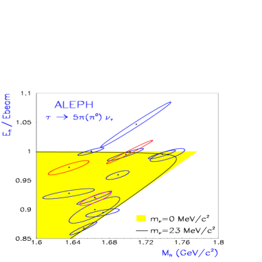
Figure 3: 2-dimensional plot of the hadronic energy versus the invariant mass of the 5(6) $\pi$-system. The error ellipses are positively correlated, because both the hadronic mass and the hadronic energy are determined from the momenta of the particles composing the hadronic system (from [36]).

Table 3: Comparision of $\nu_{\tau}$ mass limits (95 % CL) as measured by various experiments. Numbers with ^∗ include also events from 3 $\pi$-decay.

experiment	number of events	$m_{\mbox{$\nu_{\tau}$}}$ limit (MeV)
ARGUS	20	31
CLEO	266	30
OPAL	2514∗ + 5	27.6
DELPHI	6534∗	27
ALEPH	2939∗ + 41	18.2

Plans for a future charm-factory and B-factories might allow to explore $m_{\nu_{\tau}}$ down to 1-5 MeV.
Independent bounds on a possible $\nu_{\tau}$ mass in the MeV region arise from primordial nucleosynthesis in the early universe. Basically, three effects influence the detailed predictions of the abundance of light elements [37]. An unstable $\nu_{\tau}$ or its daughters would contribute to the energy density and therefore influence the Hubble-expansion. Moreover, if they decay radiatively or into $e^{+}e^{-}$ pairs, they would lower the baryon/photon ratio. A decay into final states containing $\nu_{e}$ or $\bar{\nu}_{e}$ would influence the neutron fraction and therefore the ${}^{4}He$ abundance. Recent analysis seems to rule out Dirac masses larger than 0.3 MeV and Majorana masses larger than 0.95 MeV at 95 % CL for $\nu_{\tau}$ [38]. An independent constraint from double beta decay , only valid for Majorana neutrinos, is discussed in chapter 4.1.

4 Experimental tests of the neutrino character

4.1 Double beta decay

The most promising way to distinguish between Dirac and Majorana neutrinos is neutrinoless double beta decay . For extensive reviews see [39, 40, 41]. Double beta decay was first discussed by Goeppert-Mayer [42] as a process of second order Fermi theory given by

$$(Z,A)\rightarrow(Z+2,A)+2e^{-}+2\bar{\nu_{e}}\quad(2\mbox{$\nu\beta\beta$ decay})$$ (31)

and subsequently in the form of

$$(Z,A)\rightarrow(Z+2,A)+2e^{-}\quad(0\mbox{$\nu\beta\beta$ decay})$$ (32)

first discussed by Furry [43]. Clearly, the second process violates lepton number conservation by 2 units and is only possible if neutrinos are massive Majorana particles as discussed later. In principle V+A currents could also mediate neutrinoless double beta decay , but in gauge theories both are connected and a positive signal would prove a finite Majorana mass [44, 45]. To observe double beta decay, single beta decay has to be forbidden energetically or at least strongly suppressed by large angular momentum differences between the initial and final state like in ${}^{48}Ca$ . Because of nuclear pairing energies, all possible double beta emitters are gg-nuclei and the transition is dominated by $0^{+}\rightarrow 0^{+}$ ground-state transitions. The 2$\nu\beta\beta$ decay can be seen as two subsequent Gamow-Teller transitions allowing only virtual $1^{+}$-states in the intermediate nucleus, because isospin selection rules forbid or at least strongly suppress any Fermi-transitions. The matrix elements for the 2$\nu\beta\beta$ decay can be written in the form [41]

$$M^{2\nu}_{GT}=\sum_{j}\frac{\langle 0^{+}_{f}\|t\_\sigma\|1^{+}_{j}\rangle\langle 1^{+}_{j}\|t\_\sigma\|0^{+}_{i}\rangle}{E_{j}+Q/2+m_{e}-E_{i}}$$ (33)

and for the 0$\nu\beta\beta$ decay as

$$M^{0\nu}_{GT}=\sum_{m,n}\langle 0^{+}_{f}\|t\__{m}t\__{n}H(r)\sigma_{m}\cdot\sigma_{n}\|0^{+}_{i}\rangle$$ (34)

$$M^{0\nu}_{F}=\sum_{m,n}\langle 0^{+}_{f}\|t\__{m}t\__{n}H(r)\|0^{+}_{i}\rangle(\frac{g_{V}}{g_{A}})^{2}$$ (35)

with $t\_$ as the isospin ladder operator converting a neutron into a proton, $\sigma$ as spin operator, $r=\mid\vec{r}_{m}-\vec{r}_{n}\mid$ and $H(r)$ the neutrino potential. In the neutrinoless case because of the neutrino potential also other intermediate states than $1^{+}$ might be populated [46].
Typical energies for double beta decay are in the region of a few MeV distributed among the four leptons which are therefore emitted as s-waves. The phase space depends on the available Q-value of the decay as $\propto Q^{5}$ ($0\nu\beta\beta$ decay) and $\propto Q^{11}$ ($2\nu\beta\beta$ decay), numerical values can be found in [47]. From the experimental point of view, the sum energy spectrum of the two emitted electrons has a continuous spectrum for the 2$\nu\beta\beta$ decay , while the 0$\nu\beta\beta$ decay mode results in a peak at the position corresponding to the Q-value of the involved transition (Fig.4). The single electron spectrum for the two nucleon-mechanism is given by [48]

$$(T_{1},T_{2},cos\theta)=(T_{1}+1)^{2}(T_{2}+1)^{2}\times\delta(Q-T_{1}-T_{2})(1-\beta_{1}\beta_{2}cos\theta)\quad(0\nu\beta\beta)$$ (36)

$$(T_{1},T_{2},cos\theta)=(T_{1}+1)^{2}(T_{2}+1)^{2}\times(Q-T_{1}-T_{2})^{5}(1-\beta_{1}\beta_{2}cos\theta)\quad(2\nu\beta\beta)$$ (37)

where $T_{1},T_{2}$ are the kinetic energies in units of the electron mass, $\beta_{1,2}$ is the velocity and $\theta$ the angle between the two electrons. Some favourite isotopes are given in Table 4.

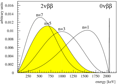
Figure 4: Different spectral shapes of observable sum energy spectra of emitted electrons in double beta decay . The n=1,3,7 forms correspond to different majoron accompanied modes, n=5 (grey) is the 2$\nu\beta\beta$ decay and the 0$\nu\beta\beta$ decay results in a peak. The energy values are taken for ${}^{76}Ge$ .

Experimental considerations

A rough estimate of the expected half-lives for the 2$\nu\beta\beta$ decay mode results in the order of $10^{20}$ years. Therefore it is an extremely rare process making low-level counting techniques necessary. To obtain reasonable chances for detection, isotopes with large phase space factors (high Q-value) and large matrix elements should be used. Also it should be possible to use a significant amount of source material, which is improved by second generation double beta decay experiments using isotopical enriched materials. One of the main concerns is possible background. Background sources are normally cosmic ray muons, man-made activities like ${}^{137}Cs$ , the natural decay chains of U and Th, cosmogenic produced unstable isotopes within the detector components, ${}^{222}Rn$ and ${}^{40}K$ . The cosmic ray muons can be shielded by going underground, the natural decay chains of U and Th are reduced by intensive selection of only very clean materials used in the different detector components, which is also valid for ${}^{40}K$ , and by using a lead shield. To avoid cosmogenics, the exposure of all detector components to cosmic rays should be minimized. This is important for semiconductor devices. ${}^{222}Rn$ can be reduced by working in an air-free environment, which can be done by using pure nitrogen. For more details on low-level counting techniques see [49].
The experiments focusing on electron detection can be either active or passive. Active detectors have the advantage that source and detector are identical as in the case of ${}^{76}Ge$ , but only measure the sum energy of both electrons. On the other hand passive detectors allow more information like measuring energy and tracks of both electrons seperately, but usually have smaller source strength. Under the assumption of a flat background in the peak region, the sensitivity for the 0$\nu\beta\beta$ half-life limit can be estimated from experimental quantities to be

$$\mbox{$T_{1/2}^{0\nu}$}\propto a\sqrt{\frac{M\cdot t}{B\cdot\Delta E}}$$ (38)

where $a$ is the isotopical abundance, $M$ the used mass, $t$ the measuring time, $\Delta E$ the energy resolution at the peak position and $B$ the background index normally given in counts/year/kg/keV. Some experiments will be described in a little more detail.
Semiconductor experiments : In this type of experiment , first done by Fiorini et al. [50], source and detector are the same, the isotope under investigation is ${}^{76}Ge$ . The big advantage is the excellent energy resolution (typically about 5 keV at 2 MeV). However, the technique only allows the measurement of the sum energy of the two electrons. A big step forward was done by using enriched germanium (natural abundance of ${}^{76}Ge$ : 7.8 %). The Heidelberg-Moscow experiment [51] in the Gran Sasso Laboratory is using 11 kg of Ge enriched to 86 % in form of five HP-detectors. A background as low as 0.2 counts/year/kg/keV at the peak position has been achieved. To improve further on background reduction, a pulse shape analysis system was developed to distinguish between single site events (like double beta decay) and multiple site events (like multiple Compton scattering) which seems to improve $B$ by another factor of five. The IGEX collaboration is using about 6 kg in form of enriched detectors [52].
Moreover, there is always the possibility to deposit a double beta decay emitter near a semiconductor detector to study the decay, but then only transitions to excited states can be observed by detecting the corresponding gamma rays.
Scintillator experiments : Some double beta decay isotopes can be used as part of scintillators. Experiments were done with ${}^{48}Ca$ in Form of CaF₂ [53] and ${}^{116}Cd$ in Form of CdWO₄ [54].
Cryogenic detectors: A technique which might become more important in the future can be bolometers running at very low temperature. Such detectors normally have a very good energy resolution. At present only one such experiment is running as a 10 mK bolometer using twenty 334g TeO₂ crystals to search for the ${}^{130}Te$ decay [55].
Ionisation experiments : These passive experiments are mostly built in form of TPCs where the emitter is either the filling gas or is included in thin foils. The advantage is that energy measurements and tracking of the two electrons is possible. Moreover, disadvantages are the energy resolution and the limited source strength by using thin foils. An experiment using a TPC with an active volume of 180 l filled with Xe (enriched to 62.5 % in ${}^{136}Xe$ which corresponds to 3.3 kg) under a pressure of 5 atm is done in the Gotthard-tunnel [56]. A TPC at UC Irvine was used to study ${}^{82}Se$ , ${}^{100}Mo$ and ${}^{150}Nd$ . A combination of drift chambers, plastic scintillators and NaI-detectors is used in the ELEGANT V detector, investigating samples of the order of 100 g enriched in ${}^{100}Mo$ and ${}^{116}Cd$ [57]. Enriched foils of ${}^{100}Mo$ , ${}^{82}Se$ , ${}^{116}Cd$ and ${}^{96}Zr$ are also used by the NEMO-2 experiment [58].
Geochemical experiments : An alternative approach relies on the detection of the daughter nucleus. The geochemical method is using very old ores, which have accumulated a significant amount of daughter nuclei. Clearly the advantage of such experiments is the long exposure time of up to a billion years. However several new uncertainties are coming into consideration like an accurate age determination, to exclude other processes producing the daughter, avoid a high initial concentration of the daughter and to have a significant source strength. From all these considerations, only Se and Te-ores are usable. ${}^{82}Se$ , ${}^{128}Te$ and ${}^{130}Te$ decay to inert noble gases (${}^{82}Kr,^{128,130}Xe$) and the detection is based on isotopical anomalies due to double beta decay which are measured by mass spectrometry [59].
Radiochemical experiments : This method takes advantage of the radioactive decay of the daughter nuclei, allowing a shorter ”measuring” time than geochemical experiments. They focus on the decay ${}^{232}Th\rightarrow^{232}U$ and ${}^{238}U\rightarrow^{238}Pu$ with Q-values of 850 keV and 1.15 MeV respectively. For the detection of the ${}^{238}U\rightarrow^{238}$Pu decay, the emission of a 5.5 MeV $\alpha$-particle from the ²³⁸Pu decay is used as a signal. Of course geo- and radiochemical methods are not able to distinguish between the different double beta decay modes and are finally limited in their sensitivity by 2$\nu\beta\beta$ decay .

2$\nu\beta\beta$ decay

The predicted half-life for the 2$\nu\beta\beta$ decay is given by

$$(\mbox{$T_{1/2}^{2\nu}$})^{-1}=G^{2\nu}(M_{GT}^{2\nu})^{2}$$ (39)

where $G^{2\nu}$ corresponds to the phase space and $M_{GT}^{2\nu}$ is the matrix element describing the transition. The main uncertainties in predicting accurate life-times are given by the errors on the matrix elements. A reliable knowledge of the matrix elements is necessary, because it influences the extractable neutrino mass limit in the 0$\nu\beta\beta$ decay as well. In the past, it was quite common to work in the closure approximation, the replacement of the energies of the virtual intermediate states by an average energy, allowing the summation over all intermediate states because $\sum\mid 1^{+}\rangle\langle 1^{+}\mid=1$. Therefore only the wavefunctions of the initial and final state have to be known. But because interference between the different contributions has to be taken into account, all amplitudes have to be weighted with the correct energy and closure fails as a good description. The present determination of the matrix elements are done with QRPA-calculations. For details see [41, 60, 61, 62]. All calculations depend on the strength of a particle-particle force which is a free parameter and has to be adjusted. A complete list of half-life calculations for A $\geq$ 70 can be found in [63].
The first evidence for double beta decay was observed in geochemical experiments using selenium and tellurium-ores [64, 65]. Newer measurements can be found in [59, 66, 67]. Because of phase space arguments, the detection of the ${}^{130}Te$ decay has to be attributed to 2$\nu\beta\beta$ decay . A radiochemical detection of double beta decay using ${}^{238}U$ with a half-life of $2.0\pm 0.6\cdot 10^{21}$ y [68] is consistent with theoretical predictions for 2$\nu\beta\beta$ decay . In 1987 the first direct laboratory detection by using ${}^{82}Se$ was reported [69]. Meanwhile 2$\nu\beta\beta$ decay has been observed in several isotopes which are listed in Table 4. The highest statistics is obtained by the Heidelberg-Moscow experiment which has observed more than 20000 events (for comparison the first observation in 1987 only consisted of 36 events).

Table 4: Compilation of observed 2$\nu\beta\beta$ decay half-lives in several isotopes. ^∗ corresponds to geochemical measurements.

Isotope	Experiment	$T_{1/2}(10^{20}y)$
48Ca	Calt.-KIAE	$0.43^{+0.24}_{-0.11}\pm 0.14$
76Ge	MPIK-KIAE	17.7 $\pm 0.1^{+1.3}_{-1.1}$
76Ge	IGEX	11 $\pm$ 1.5
82Se	NEMO 2	$0.83\pm 0.10\pm 0.07$
100Mo	ELEGANT V	$0.115^{+0.03}_{-0.02}$
100Mo	NEMO 2	0.095 $\pm$ 0.004 $\pm$ 0.009
100Mo	UCI	$0.0682^{+0.0038}_{-0.0053}\pm$ 0.0068
${}^{116}Cd$	NEMO 2	0.375 $\pm$ 0.035 $\pm$ 0.021
${}^{116}Cd$	ELEGANT V	$0.26^{+0.09}_{-0.05}$
128Te∗	Wash. Uni-Tata	77000 $\pm$ 4000
150Nd	ITEP/INR	$0.188^{+0.066}_{-0.039}\pm 0.019$
150Nd	UCI	$0.0675^{+0.0037}_{-0.0042}\pm 0.0068$

0$\nu\beta\beta$ decay

The half-life for the 0$\nu\beta\beta$ decay is given by (assuming $m_{\nu}\mbox{$\stackrel{{\scriptstyle<}}{{\sim}}$ }$ 1 MeV)

$$(\mbox{$T_{1/2}^{0\nu}$})^{-1}=G^{0\nu}(M_{GT}-M_{F})^{2}\left(\frac{\mbox{$\langle m_{\nu_{e}}\rangle$ }}{m_{e}}\right)^{2}$$ (40)

where the effective Majorana neutrino mass $\langle m_{\nu_{e}}\rangle$ is given by

$$\mbox{$\langle m_{\nu_{e}}\rangle$ }=\mid\sum_{i}U_{ei}^{2}\eta_{i}m_{i}\mid$$ (41)

with the relative CP-phases $\eta_{i}=\pm 1$, $U_{ei}$ as the mixing matrix elements and $m_{i}$ as the corresponding mass eigenvalues. The expression can be generalised if right-handed currents are included to

$$(\mbox{$T_{1/2}^{0\nu}$})^{-1} = C_{mm}(\frac{\mbox{$\langle m_{\nu_{e}}\rangle$ }}{m_{e}})^{2}+C_{\eta\eta}\langle\eta\rangle^{2}+C_{\lambda\lambda}\langle\lambda\rangle^{2}$$

$$+C_{m\eta}(\frac{\mbox{$\langle m_{\nu_{e}}\rangle$ }}{m_{e}})\langle\eta\rangle+C_{m\lambda}(\frac{\mbox{$\langle m_{\nu_{e}}\rangle$ }}{m_{e}})\langle\lambda\rangle+C_{\eta\lambda}\langle\eta\rangle\langle\lambda\rangle$$

where the coefficients C contain the phase space factors and the matrix elements,

$$\langle\eta\rangle=\eta\sum_{j}U_{ej}V_{ej}\quad\langle\lambda\rangle=\lambda\sum_{j}U_{ej}V_{ej}$$ (42)

with $V_{ej}$ as the mixing matrix elements between right-handed neutrinos. Eq.(4.1) reduces to eq.(40) in case $\langle\eta\rangle,\langle\lambda\rangle$ = 0. Also in 0$\nu\beta\beta$ decay the matrix element calculations are done with QRPA-calculations [63, 70, 71, 72]. The general agreement between the calculations done by different groups are within a factor 2-3.
From the experimental point, the evidence for 0$\nu\beta\beta$ decay in the sum energy spectrum of the electrons is a peak at the position corresponding to the Q-value of the involved transition. The half-life limits obtained so far for several different isotopes are shown in Table 5. The best limit is coming from the Heidelberg-Moscow experiment resulting in a bound of [74] (Fig.5)

$$\mbox{$T_{1/2}^{0\nu}$}>1.1\cdot 10^{25}y\rightarrow\mbox{$\langle m_{\nu_{e}}\rangle$ }<0.47eV\quad(90\%CL)$$ (43)

using the matrix elements of [63]. Because in most see-saw models $\langle m_{\nu_{e}}\rangle$ corresponds to $m_{\nu_{e}}$ [10] (see Table 1), this bound is much stronger than single beta decay but applies only if neutrinos are Majorana particles.

Table 5: Compilation of neutrinoless double beta decay half-life and mass limits of the most investigated isotopes. The phase space factors and Q-values are taken from [47]. ^‡ after [73], ^∗ corresponds to geochemical measurement.

Decay	Q-value (keV)	(G${}^{0\nu})^{-1}(y)$	$T_{1/2}^{0\nu}$ (y)	$\langle m_{\nu}\rangle$ (eV)
${}_{20}^{48}$Ca$\rightarrow_{22}^{48}$Ti	4271 $\pm$ 4	4.10E24	$>9.5\cdot 10^{21}(76\%)$	$<12.8(76\%)^{\ddagger}$
${}_{32}^{76}$Ge$\rightarrow_{34}^{76}$Se	2039.6 $\pm$ 0.9	4.09E25	$>1.1\cdot 10^{25}\hfill(90\%)$	$<0.5\hfill(90\%)$
${}_{34}^{82}$Se$\rightarrow_{36}^{82}$Kr	2995 $\pm$ 6	9.27E24	$>2.7\cdot 10^{22}\hfill(68\%)$	$<5.0\hfill(68\%)$
${}_{~{}42}^{100}$Mo$\rightarrow_{~{}44}^{100}$Ru	3034 $\pm$ 6	5.70E24	$>5.2\cdot 10^{22}\hfill(68\%)$	$<5.0\hfill(68\%)$
${}_{~{}48}^{116}$Cd$\rightarrow_{~{}50}^{116}$Sn	2802 $\pm$ 4	5.28E24	$>2.9\cdot 10^{22}\hfill(90\%)$	$<4.1\hfill(90\%)$
${}_{~{}52}^{128}$Te$\rightarrow_{~{}54}^{128}$Xe	868 $\pm$ 4	1.43E26	$>7.7\cdot 10^{24}\hfill(68\%)$	$<1.1\hfill(68\%)^{\ast}$
${}_{~{}52}^{130}$Te$\rightarrow_{~{}54}^{130}$Xe	2533 $\pm$ 4	5.89E24	$>5.6\cdot 10^{22}\hfill(90\%)$	$<3.0\hfill(90\%)$
${}_{~{}54}^{136}$Xe$\rightarrow_{~{}56}^{136}$Ba	2479 $\pm$ 8	5.52E24	$>4.4\cdot 10^{23}\hfill(90\%)$	$<2.3\hfill(90\%)$
${}_{~{}60}^{150}$Nd$\rightarrow_{~{}62}^{150}$Sm	3367.1 $\pm$ 2.2	1.25E24	$>2.1\cdot 10^{21}\hfill(90\%)$	$<4.1\hfill(90\%)$

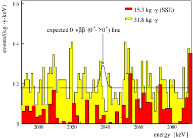
Figure 5: Observed spectrum near the expected 0$\nu\beta\beta$ decay peak of the Heidelberg-Moscow collaboration. No signal can be seen. The two different spectra correspond to measuring periods with (black) and without (grey) pulse shape discrimination (with kind permission of H.V. Klapdor-Kleingrothaus).

Allowing also right-handed currents to contribute, $\langle m_{\nu_{e}}\rangle$ is fixed by an ellipsoid which is shown in Fig. 6. As can be seen, the largest mass allowed occurs for $\langle\lambda\rangle,\langle\eta\rangle\neq 0$. In this case the half-life of eq. 43 corresponds to

$$\mbox{$\langle m_{\nu_{e}}\rangle$ }<0.56eV$$ (44)

$$\langle\eta\rangle<6.5\cdot 10^{-9}$$ (45)

$$\langle\lambda\rangle<8.2\cdot 10^{-7}$$ (46)

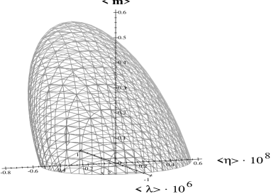
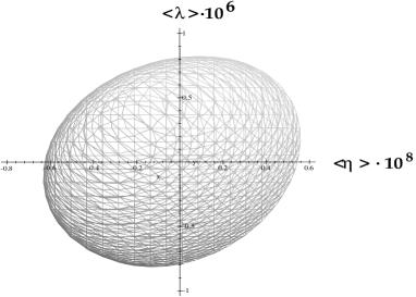
Figure 6: Obtained neutrino mass $\langle m_{\nu_{e}}\rangle$ as a function of the two right-handed current parameters $\langle\lambda\rangle,\langle\eta\rangle$. On the right the projection on the $\langle\lambda\rangle,\langle\eta\rangle$ plane is shown.

The limit also allows a bound on a possible right-handed $W_{R}$ which is shown in Fig. 7. Together with vacuum stability arguments a mass for $W_{R}$ lower than about 1 TeV can be excluded. The influence of double charged Higgses, which also can contribute to neutrinoless double beta decay is shown as well [75].

Figure 7: Bound on the mass of a right-handed W as a function of the heavy neutrino mass $m_{N}$. under the assumption of different masses of the double charged higgs $\Delta^{--}$. Shown are the regions excluded by double beta decay (lower left) and from vacuum stability (lower right). The curves a-e correspond to masses of 0.3 TeV, 1 TeV, 2 TeV, 5 TeV and infinite for the $\Delta^{--}$ (from [75]).

Limits on other interesting quantities like the R-parity violating SUSY parameter $\lambda^{\prime}_{111}$ [76] and leptoquarks [77] can be derived. From the point of right-handed currents the investigation of the transition to the first excited state is important, because the mass term here vanishes in first order. The phase space for this transition is smaller, but the de-excitation photon might allow a good experimental signal. For a compilation of existing bounds on transitions to excited states see [78]. As long as no signal is seen, bounds from ground state transitions are much more stringent on right-handed parameters.
Eq.(41) has to be modified in case of heavy neutrinos ($m_{\nu}\mbox{$\stackrel{{\scriptstyle>}}{{\sim}}$ }$1 MeV). For such heavy neutrinos the mass can no longer be neglected in the neutrino propagator resulting in an A-dependent contribution

$$\mbox{$\langle m_{\nu_{e}}\rangle$ }=\mid\sum_{i=1,light}^{N}U^{2}_{ei}m_{i}+\sum_{h=1,heavy}^{M}F(m_{h},A)U^{2}_{eh}m_{h}\mid$$ (47)

By comparing these limits for isotopes with different atomic mass, interesting limits on the mixing angles and $\nu_{\tau}$ parameters for an MeV $\nu_{\tau}$ can be obtained [79, 80].
A complete new class of decays emerges in connection with majoron emission in double beta decay [81]. The majoron $\chi$ is the Goldstone-boson of a spontaneous breaking of a global lepton-number symmetry. Depending on its transformation properties under weak isospin, singlet [82], doublet [83] and triplet [84] models exist. The triplet and pure doublet model are excluded by the measurements of the Z-width at LEP, because they would contribute 2 (triplet) or 0.5 (doublet) neutrino flavours. Several new majoron-models evolved during the last years [85, 86]. In consequence different spectral shapes for the sum electron spectrum are predicted which can be written as

$$\frac{dN}{dE}\propto(Q-E)^{n}\cdot F(E,Z)$$ (48)

where F(E,Z) is the Fermi-function and the spectral index $n$ is 1 for the classical majoron, n=3 for lepton number carrying majorons, n=5 for 2$\nu\beta\beta$ decay and n=7 for several other majoron models. A different shape is obtained in the vector majoron picture of Carone [87]. It should be noted that supersymmetric Zino-exchange allows the emission of two majorons, which also results in n=3, but a possible bound on a Zino-mass is less stringent than direct accelerator experiments [88]. In the n=1 model the effective neutrino -majoron coupling $\langle g_{\nu\chi}\rangle$ can be deduced from

$$(T_{1/2}^{0\nu\chi})^{-1}=\mid M_{GT}-M_{F}\mid^{2}G^{0\nu\chi}\mid\langle g_{\nu\chi}\rangle\mid^{2}$$ (49)

where $\langle g_{\nu\chi}\rangle$ is given by

$$\langle g_{\nu\chi}\rangle=\sum_{i,j}g_{\nu\chi}U_{ei}U{ej}$$ (50)

Present half-life limits for this decay (n=1) and the deduced coupling constants are given in Table 6. A first half-life limit for the n=3 mode was given in [89], a evaluation for ${}^{100}Mo$ is given in [90]. A more recent extensive study of all modes can be found in [86]. Limits obtained by the Heidelberg-Moscow experiment with a statistical significance of 4.84 kg$\cdot$y are [91]

$$T_{1/2}^{0\nu\chi}>5.85\cdot 10^{21}y\quad\mbox{(n=3)}$$ (51)

$$T_{1/2}^{0\nu\chi}>6.64\cdot 10^{21}y\quad\mbox{(n=7)}$$ (52)

Table 6: Compilation of limits on half-lives and effective majoron-neutrino couplings from different isotopes. ^∗ corresponds to a geochemical measurement, which has no power to discriminate between different decay modes.

Isotope	Experiment	$T_{1/2}(10^{21}y)$	$\langle g_{\nu\chi}\rangle(10^{-4})$
48Ca	ITEP	0.72 (90 %)	5.3
76Ge	MPIK-KIAE	7.91 (90 %)	2.3
76Ge	ITEP	10 (68 %)	2.2
76Ge	UCSB-LBL	1.4 (90 %)	5.8
76Ge	PNL-USC	6.0	2.8
76Ge	Cal.-PSI-Neu	1.0 (90 %)	6.9
82Se	NEMO 2	2.4 (90 %)	1.4
100Mo	ELEGANT V	5.4 (68 %)	0.7
100Mo	NEMO 2	0.5 (90 %)	2.3
100Mo	UCI	0.3 (90 %)	3
128Te∗	Wash. Uni-Tata	7700	0.3
136Xe	Cal.-PSI-Neu	14 (90 %)	1.5
150Nd	UCI	0.28 (90 %)	1

Additionally the $\beta^{+}\beta^{+}$-decay in combination with EC can be observed via the following decay modes

$$(Z,A)\rightarrow(Z-2,A)+2e^{+}+(2\mbox{$\nu_{e}$})$$ (53)

$$e_{B}^{-}+(Z,A)\rightarrow(Z-2,A)+e^{+}+(2\mbox{$\nu_{e}$})$$ (54)

$$2e_{B}^{-}+(Z,A)\rightarrow(Z-2,A)+2\mbox{$\nu_{e}$}$$ (55)

$$2e_{B}^{-}+(Z,A)\rightarrow(Z-2,A)^{\ast}\rightarrow(Z-2,A)+\gamma+2\mbox{X-rays}$$ (56)

$\beta^{+}\beta^{+}$ is always accompanied by EC/EC or $\beta^{+}$/EC-decay. Because of the Coulomb-barrier and the reduction of the Q-value by 4 $m_{e}c^{2}$, the rate for $\beta^{+}\beta^{+}$ is small and energetically only possible for seven nuclides. Predicted half-lives for $\beta^{+}\beta^{+}$ are of the order $10^{26}$ y while for $\beta^{+}$/EC this can be reduced by orders of magnitude down to $10^{22-23}$ y making an experimental detection more realistic. The experimental signature of the decay modes is rather clear because of the two or four 511 keV photons. The last mode (eq.56) to an excited state is giving a characteristic gamma associated with X-ray emission. Half-lives obtained with ¹⁰⁶Cd and ${}^{96}Ru$ are of the order $10^{18}$ y [92, 78]. Extracted neutrino mass limits are orders of magnitude worse than the 0$\nu\beta\beta$ decay limits, but if there is any positive observation of the 0$\nu\beta\beta$ decay mode, the $\beta^{+}$/EC-mode can be used to distinguish whether this is dominated by the neutrino mass mechanism or right-handed currents [93].

Future

Several upgrades are planned to improve the existing half-life limits. Because of the enormous source strength after additional years of running the dominant project will still be the Heidelberg-Moscow experiment probing neutrino masses down to 0.2 eV. A new experiment to improve the sensitivity on ${}^{48}Ca$ is ELEGANT VI, using 25 modules of $CaF_{2}$ with a total amount of 31 g of ${}^{48}Ca$ within a CsI detector [57]. A different approach might be the use of $CaF_{2}(Eu)$ as a cryogenic bolometer and to measure simultaneously the scintillation light [94]. ${}^{48}Ca$ is interesting because it can be treated with nuclear shell model calculations. The building up of NEMO-3, which should start operation in 1999, will allow to use up to 10 kg of material in form of foils for several isotopes like ${}^{100}Mo$ [95]. Even more ambitious would be the usage of large amounts of materials (in the order of several hundred kg to tons) like enriched ${}^{136}Xe$ added to scintillators [96], 750 kg $TeO_{2}$ in form of cryogenic bolometers (CUORE) [97] or a huge cryostat containing several hundred detectors of enriched ${}^{76}Ge$ with a total mass of 1 ton (GENIUS) [98]. Further, ideas to use a large amount of ${}^{136}Xe$ and detect the created daughter ¹³⁶Ba with atomic traps and resonance ionisation spectroscopy exist. This will allow no information on the decay mode and will be dominated by 2$\nu\beta\beta$ decay [99, 100].

4.2 Magnetic moment of the neutrino

Another possibility to check the neutrino character is the search for its magnetic moment . In the present standard model both types of neutrinos have no magnetic moment because neutrinos are massless and a magnetic moment would require a coupling of a left-handed state with a right-handed one which is absent. A simple extension by including right-handed singlets allows for Dirac-masses. In this case, it can be shown that neutrinos can get a magnetic moment due to loop diagrams which is proportional to their mass and is given by [101, 102]

$$\mbox{$\mu_{\nu}$}=\frac{3G_{F}e}{8\sqrt{2}\pi^{2}}m_{\nu}=3.2\cdot 10^{-19}(\frac{m_{\nu}}{eV})\mbox{$\mu_{B}$}$$ (57)

In case of neutrino masses in the eV-range, this is far to small to be observed and to have any significant effects in astrophysics. Nevertheless there exist GUT-models, which are able to increase the magnetic moment without increasing the mass [103]. However Majorana neutrinos still have a vanishing static moment because of CPT-invariance. The existence of diagonal terms in the magnetic moment matrix would therefore prove the Dirac-character of neutrinos . Non-diagonal terms in the moment matrix are possible for both types of neutrinos allowing transition moments of the form $\nu_{e}$ - $\bar{\nu}_{\mu}$.
Limits on magnetic moments arise from $\nu_{e}$ $e$ - scattering experiments and astrophysical considerations. The differential cross section for $\nu_{e}$ $e$ - scattering in presence of a magnetic moment is given by

$$\frac{d\sigma}{dT}=\frac{G_{F}^{2}m_{e}}{2\pi}[(g_{V}+x+g_{A})^{2}+(g_{V}+x-g_{A})^{2}(1-\frac{T}{E_{\nu}})^{2}$$ (58)

$$+(g_{A}^{2}-(x+g_{V})^{2})\frac{m_{e}T}{E_{\nu}^{2}}]+\frac{\pi\alpha^{2}\mbox{$\mu_{\nu}$}^{2}}{m_{e}^{2}}\frac{1-T/E_{\nu}}{T}$$ (59)

where T is the kinetic energy of the recoiling electron and

$$g_{V}=2sin^{2}\theta_{W}+\frac{1}{2}\quad g_{A}=\pm\frac{1}{2}\quad(+(-)\quad\mbox{for}\quad\mbox{$\nu_{e}$}(\bar{\mbox{$\nu_{e}$}}))$$ (60)

and $x$ denotes the neutrino form factor related to its square charge radius $\langle r^{2}\rangle$

$$x=\frac{2m_{W}^{2}}{3}\langle r^{2}\rangle sin^{2}\theta_{W}\quad x\rightarrow-x\quad for\quad\bar{\mbox{$\nu_{e}$}}$$ (61)

The contribution associated with the charge radius can be neglected in the case $\mu_{\nu}\stackrel{{\scriptstyle>}}{{\sim}}10^{-11}\mbox{$\mu_{B}$}$. As can be seen, the largest effect of a magnetic moment can be observed in the low energy region, and because of destructive interference of the electroweak terms, searches with antineutrinos would be preferred. The obvious sources are therefore nuclear reactors. Experiments done so far result in a bound of $\mbox{$\mu_{\nu}$}<1.52\cdot 10^{-10}\mbox{$\mu_{B}$}$ for $\bar{\nu}_{e}$ [104]. Measurements based on $\nu_{e}$ $e\rightarrow\mbox{$\nu_{e}$}e$ and $\nu_{\mu}$ $e\rightarrow\mbox{$\nu_{\mu}$}e$ scattering were done at LAMPF and BNL yielding bounds for $\nu_{e}$ and $\nu_{\mu}$ of $\mu_{\nu}\stackrel{{\scriptstyle<}}{{\sim}}10^{-9}\mbox{$\mu_{B}$}$ [105, 106].
Astrophysical limits are somewhat more stringent but also more model dependent. An explanation of the solar neutrino problem by spin precession of $\nu_{L}$ into $\nu_{R}$ done by the magnetic field of the solar convection zone requires a magnetic moment of the order $\mu_{\nu}$ $\approx 10^{-10}-10^{-11}\mbox{$\mu_{B}$}$ [107]. Observation of neutrinos from Supernova 1987A yield a somewhat model dependent bound of $\mu_{\nu}$ $<10^{-12}\mbox{$\mu_{B}$}$ [108, 109]. Also the neutrino emissivity of globular cluster stars done by excessive plasmon decay $\gamma\rightarrow\nu\bar{\nu}$ is only consistent with observation for a magnetic moment of the same order [110]. This last bound applies to neutrinos lighter than 5 keV.
To improve the experimental situation and especially check the region relevant for the solar neutrino problem new experiments are under construction. The most advanced is the NUMU experiment [111] currently installed near the Bugey reactor. It consists of a 1 m³ TPC loaded with CF₄ under a pressure of 5 bar. The usage of a TPC will not only allow to measure the electron energy but for the first time in such experiments also the scattering angle, therefore allowing the reconstruction of the neutrino energy. The neutrino energy spectrum at reactors in the energy region 1.5 $<E_{\nu}<$ 8 MeV is known at the 3 % level. To suppress background, the TPC is surrounded by 50 cm anti-Compton scintillation detectors as well as a passive shielding of lead and polyethylene. In case of no magnetic moment the expected count rate is 9.5 per day increasing to 13.4 per day if $\mbox{$\mu_{\nu}$}=10^{-10}\mbox{$\mu_{B}$}$ for an energy threshold of 500 keV. The estimated background is 6 events per day. The expected sensitivity level is down to $\mbox{$\mu_{\nu}$}=3\cdot 10^{-11}\mbox{$\mu_{B}$}$ . The usage of a low background Ge-NaI spectrometer in a shallow depth near a reactor has also been considered [112]. The usage of large low-level detectors with a low-energy threshold of a few keV in underground laboratories is also under investigation. The reactor would be replaced by a strong $\beta$-source. Calculations for a scenario of a 1-5 MCi ¹⁴⁷Pm source (endpoint energy of 234.7 keV) in combination with a 100 kg low-level NaI(Tl) detector with a threshold of about 2 keV can be found in [113].

4.3 Search for heavy Majorana neutrinos

For the see-saw-mechanism to work heavy Majorana neutrinos N are necessary. The required lightness of neutrino masses makes a detection of the corresponding heavy state impossible. The mixing of a heavy neutrino $m_{H}$ to the light state $m_{L}$ is ruled by $\theta=\sqrt{m_{L}/m_{H}}\ll 1$. However there exist theoretical models which decouple the mixing from any mass relation [114, 115]. Assuming that in eq.(3) $m_{L}^{M}\neq 0$ and that by an internal symmetry at tree level the relation $m_{L}^{M}m_{R}^{M}=(m^{D})^{2}$ is valid, the mixing is decoupled from the ratio $m_{1}/m_{2}$ and can be close to one in case that $m_{L}^{M}\approx m_{R}^{M}$. Masses for light neutrinos vanish at tree level and will be generated at higher orders.
From the experimental point of view, heavy Majorana neutrinos can be searched for at accelerators. The LEP-data on the $Z^{o}$-width already exclude any additional neutrino lighter than 45 GeV. Searches for heavier neutrinos have been done at LEP1.5. The search for Majorana neutrinos heavier than the $Z^{o}$ focusses on the N-decay channels

$$N\rightarrow e^{\pm}W^{\mp}\quad and\quad N\rightarrow\nu Z^{o}$$ (62)

which is identical to signatures looked for in searches of excited fermions. A detailed description of pair production of heavy Dirac and Majorana neutrinos in $e^{+}e^{-}$collisions can be found in [116]. Pair production of Majorana neutrinos would result in two like-sign charged leptons. Furthermore, HERA offers the chance to search for heavy Majorana masses in ep-collisions [117]. For accumulated 200 $pb^{-1}$ a discovery limit up to 160 GeV is possible. Also future high energy $e^{+}e^{-}$ machines allow an extended search for heavy neutrinos via reactions

$$e^{+}e^{-}\rightarrow\nu N\quad N\rightarrow e^{\pm}W^{\mp},N\rightarrow\nu Z,N\rightarrow\nu H$$ (63)

The dominant background will be $W^{+}W^{-}$production [118]. LHC offers searches either in the pair-production or single Majorana neutrino production mode [119, 120, 121]. The advantage of single Majorana production is that it depends only linearly on the neutrino mixing. The single production channel via

$$pp\rightarrow e^{-}NX\rightarrow e^{-}e^{-}W^{+}X$$ (64)

offers a signal of two same sign leptons, two jets with the invariant mass of $m_{W}^{2}$ and no missing energy. For an assumed luminosity of 10 fb^-1 the discovery potential goes up to 1.4 TeV (0.8 TeV) for an assumed mixing of $sin\theta\approx 10^{-2}(10^{-3})$.

5 Neutrino oscillations

In case of massive neutrinos the mass eigenstates do not have to be identical with the flavour eigenstates, similar to the CKM-mixing in the quark sector. This offers the chance for neutrino oscillations. Oscillations might be the only chance to see effects of $\nu_{\mu}$ and $\nu_{\tau}$ in the eV mass range which is not accessible in direct experiments.

5.1 General formalism

The concept of neutrino oscillations has been introduced by [122]. The weak eigenstates $\nu_{\alpha}$ are related to the mass eigenstates $\nu_{i}$ via a unitary matrix U

$$\nu_{\alpha}=\sum_{i}U_{\alpha i}\nu_{i}$$ (65)

which is given for Dirac neutrinos as

$$U=\left(\begin{array}[]{ccc}c_{12}c_{13}&s_{12}c_{13}&s_{13}e^{-i\delta}\\ -s_{12}c_{23}-c_{12}s_{23}s_{13}e^{i\delta}&c_{12}c_{23}-s_{12}s_{23}s_{13}e^{i\delta}&s_{23}c_{13}\\ s_{12}s_{23}-c_{12}s_{23}s_{13}e^{i\delta}&-c_{12}s_{23}-s_{12}c_{23}s_{13}e^{i\delta}&c_{23}c_{13}\end{array}\right)$$ (66)

and in the Majorana case as

$$U=\left(\begin{array}[]{ccc}c_{12}c_{13}&s_{12}c_{13}e^{-i\delta_{12}}&s_{13}e^{-i\delta_{13}}\\ -s_{12}c_{23}e^{i\delta_{12}}-c_{12}s_{23}s_{13}e^{i(\delta_{13}+\delta_{23})}&c_{12}c_{23}-s_{12}s_{23}s_{13}e^{i(\delta_{23}+\delta_{13}-\delta_{12})}&s_{23}c_{13}e^{i\delta_{23}}\\ s_{12}s_{23}e^{i(\delta_{13}+\delta_{23})}-c_{12}s_{23}s_{13}e^{i(\delta_{13}+\delta_{23})}&-c_{12}s_{23}e^{i\delta_{23}}-s_{12}c_{23}s_{13}e^{i(\delta_{13}-\delta_{12})}&c_{23}c_{13}\end{array}\right)$$ (67)

with $c,s=cos\theta,sin\theta$. The quantum mechanical transition probability can be derived (assuming relativistic neutrinos and CP-conservation) as [7]

$$P(\nu_{\alpha}\rightarrow\nu_{\beta})=\sum_{i}\mid U_{\beta i}\mid^{2}\mid U_{\alpha i}\mid^{2}+Re\sum_{i\neq j}U_{\beta i}U^{\ast}_{\beta j}U^{\ast}_{\alpha i}U_{\alpha j}exp(-it\mbox{$\Delta m^{2}$}_{ij}/2E)$$ (68)

with $\mbox{$\Delta m^{2}$}_{ij}=\mid m_{i}^{2}-m_{j}^{2}\mid$. In the simple two-flavour mixing the probability to find $\nu_{\beta}$ in a distance $x$ with respect to a source of $\nu_{\alpha}$ is given by

$$P(\nu_{\alpha}\rightarrow\nu_{\beta})=\mbox{$sin^{2}2\theta$}sin^{2}\frac{\pi x}{L}$$ (69)

giving the oscillation length L in practical units as

$$L=\frac{4\pi E\hbar}{\mbox{$\Delta m^{2}$}c^{3}}=2.48(\frac{E}{MeV})(\frac{eV^{2}}{\mbox{$\Delta m^{2}$}})\quad m$$ (70)

For a more extensive review on N flavour mixing, wave-packet treatment and coherence considerations see [7, 123, 124]. Terrestrial experiments are done with nuclear reactors and accelerators. The discussed oscillation searches involve the three known neutrinos as well as a possible sterile neutrino $\nu_{S}$.

5.2 Reactor experiments

Reactor experiments are disappearance experiments looking for $\bar{\nu}_{e}$ $\rightarrow\bar{\nu}_{X}$.

5.2.1 Principles

Reactors are a source of MeV $\bar{\nu}_{e}$ due to the fission of nuclear fuel. The main isotopes involved are ²³⁵U,²³⁸U,²³⁹Pu and ²⁴¹Pu. The neutrino rate per fission has been measured [126] for all isotopes except ²³⁸U and is in good agreement with theoretical calculations [127]. Experiments typically try to measure the positron spectrum which can be deduced from the $\bar{\nu}_{e}$ - spectrum and either compare it directly to the theoretical predictions or measure it at several distances from the reactor and search for spectral changes. Both types of experiments were done in the past. The $\bar{\nu}_{e}$ cross section is known to about 1.4 % [128]. The detection reaction is

$$\mbox{$\bar{\nu}_{e}$}+p\rightarrow e^{+}+n$$ (71)

with an energy threshold of 1.804 MeV. The detection reaction (71) is always the same, resulting in different strategies for the detection of the positron and the neutron. Normally coincidence techniques are used between the annihilation photons and the neutrons which diffuse and thermalise within 10-100 $\mu$s. The main background are cosmic ray muons producing neutrons in the surrounding of the detector.

5.2.2 Experimental status

Several reactor experiments have been done in the past (see Table 7). All these experiments had a fiducial mass of less than 0.5 t and the distance to the reactor was never more than 250 m.

Table 7: List of finished reactor experiments. Given are the power of the reactors and the distance of the experiments with respect to the reactor.

reactor	thermal power [MW]	distance [m]
ILL-Grenoble (F)	57	8.75
Bugey (F)	2800	13.6, 18.3
Rovno (USSR)	1400	18.0,25.0
Savannah River (USA)	2300	18.5,23.8
Gösgen (CH)	2800	37.9, 45.9, 64.7
Krasnojarsk (Russia)	?	57.0, 57.6, 231.4
Bugey III (F)	2800	15.0, 40.0, 95.0

Two new reactor experiments producing data are CHOOZ and Palo Verde. The CHOOZ-experiment in France [129] has some advantages with respect to previous experiments. First of all the detector is located underground with a shielding of 300 mwe, reducing the background due to atmospheric muons by a factor of 300. Moreover, the detector is about 1030 m away from two 4.2 GW reactors (more than a factor 4 in comparison to previous experiments) enlarging the sensitivity to smaller $\Delta m^{2}$ . In addition the main target has about 4.8 t and is therefore much larger than those used before. The main target consists of a specially developed Gd-loaded scintillator. This inner detector is surrounded by an additional detector containing 17 t of scintillator without Gd and 90 t of scintillator as an outer veto. The signal in the inner detector is the detection of the annihilation photons in coincidence with n-capture on Gd, the latter producing gammas with a total sum of up to 8 MeV. The first published positron spectrum [130] is shown in Fig. 8 and shows no hints for oscillations. The resulting exclusion plot is shown in Fig.18.

Figure 8: The measured positron spectrum of the CHOOZ-experiment (left). On the right the ratio with the expectation is shown. No oscillation signal is visible (from [130]).

The second experiment is the Palo Verde (former San Onofre) experiment [131] near Phoenix, AZ (USA). It consists of 12 t liquid scintillator also loaded with Gd. The scintillator is filled in 66 modules arranged in an 11$\times$6 array. The coincidence of three modules serves as a signal. The experiment is located under a shielding of 46 mwe in a distance of about 750 (820) m to three reactors with a total power of 10.2 GW.
A further project plans a 1000 t liquid scintillator detector (KamLAND) [132]. It is approved by the Japanese Government and will be constructed at the Kamioka site. Having a distance of 160 km to the next reactor, it will probe $\Delta m^{2}$ down to $10^{-5}eV^{2}$.

5.3 Accelerator experiments

The second source of terrestrial neutrinos are high energy accelerators. Experiments can be of either appearance or disappearance type [125].

5.3.1 Principles

Accelerators typically produce neutrino beams by shooting a proton beam on a fixed target. The produced secondary pions and kaons decay and create a neutrino beam dominantly consisting of $\nu_{\mu}$ . The detection mechanism is via charged weak currents

$$\nu_{i}N\rightarrow i+X\quad i=e,\mu,\tau$$ (72)

where N is a nucleon and X the hadronic final state. Depending on the intended goal, the search for oscillations therefore requires a detector which is capable of detecting electrons, muons and $\tau$ - leptons in the final state.

5.3.2 Experimental status

Accelerators at medium energy

At present there are two experiments running with neutrinos at medium energies ($E_{\nu}\approx$ 30 - 50 MeV) namely KARMEN and LSND . Both experiments use 800 MeV proton beams on a beam dump to produce pions. The expected neutrino spectrum from pion and $\mu$-decay is shown in Fig. 9. The beam contamination of $\bar{\nu}_{e}$ is in the order of $10^{-4}$.

Figure 9: Neutrino spectrum from $\pi$-decay. Beside the monoenergetic line from $\pi^{+}$-decay at rest, the continuous spectra of $\nu_{e}$ and $\bar{\nu}_{\mu}$ are shown.

The KARMEN experiment [133] at the neutron spallation source ISIS at Rutherford Appleton Laboratory is using 56 t of a segmented liquid scintillator. The main advantage of this experiment is the known time structure of the two proton pulses hitting the beam dump (two pulses of 100 ns with a separation of 330 ns and a repetition rate of 50 Hz). Because of the pulsed beam, positrons are expected within 0.5-10.5 $\mu$s after beam on target. The signature for detection is a delayed coincidence of a positron in the 10 - 50 MeV region together with $\gamma$-emission from either p(n,$\gamma$)D or Gd(n,$\gamma$)Gd reactions. The first results in 2.2 MeV photons while the latter allows gammas up to 8 MeV. The limit reached so far is shown in Fig. 10. Recently KARMEN published a 2- and 3- flavour analysis of $\nu_{e}$ -$\nu_{\tau}$ and $\nu_{e}$ - $\nu_{\mu}$ oscillations by comparing the energy averaged CC-cross section for $\nu_{e}$ interactions with expectation as well as making a detailed maximum likelihood analysis of the spectral shape of the electron spectrum observed from ${}^{12}C$ ($\nu_{e}$ ,e^-)${}^{12}N$ _gs reactions [134]. To improve the sensitivity by reducing the neutron background, a new veto shield against atmospheric muons was constructed which has been in operation since Feb. 1997 and is surrounding the whole detector. The region which can be investigated in 2-3 years of running in the upgraded version is also shown in Fig. 10.

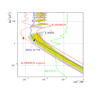
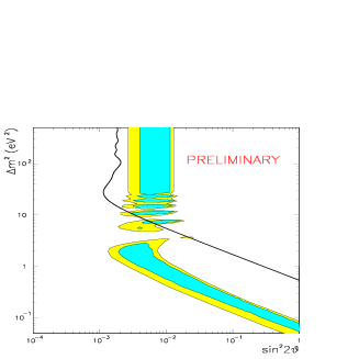
Figure 10: $\nu_{e}$ - $\nu_{\mu}$ parameter plot. Shown is the region of evidence from the LSND $\pi$-decay at rest analysis (grey areas) and different exclusion curves from Bugey, KARMEN, E776 (left) and the preliminary NOMAD result (right).

The LSND experiment [135] at LAMPF is a 167 t mineral oil based liquid scintillation detector using scintillation and Cerenkov light for detection. It consists of an approximately cylindrical tank 8.3 m long and 5.7 m in diameter. The experiment is about 30 m away from a copper beam stop under an angle of 12^o with respect to the proton beam. For the oscillation search in the channel $\bar{\nu}_{\mu}$ -$\bar{\nu}_{e}$ a signature of a positron within the energy range 36 MeV $<E_{e}<$ 60 MeV together with an in time and spatial correlated 2.2 MeV photon from p(n,$\gamma$)D is required. The analysis (Fig. 11) [136] ends up in evidence for oscillations in the region shown in Fig.10.

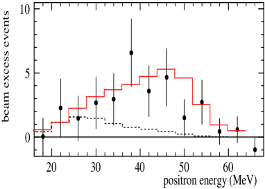
Figure 11: Positron spectrum of beam-excess data. The dashed curve corresponds to the estimated neutrino background while the solid line indicates neutrino oscillations for large $\Delta m^{2}$ plus the estimated background (from [136]).

Recently LSND published their $\nu_{e}$ - $\nu_{\mu}$ analysis for pion decays in flight by looking for isolated electrons in the region 60 MeV $<E_{e}<$ 200 MeV coming from ${}^{12}C$ ($\nu_{e}$ ,e^-)${}^{12}N$ _gs reactions [137], which is in agreement with the former evidence from pion decay at rest. Also LSND continues with data acquisition.
An increase in sensitivity in the $\nu_{\mu}$ - $\nu_{e}$ oscillation channel can be reached in the future if there is a possibility for neutrino physics at the planned European Spallation Source (ESS) or the National Spallation Neutron Source (NSNS) at Oak Ridge which might have a 1 GeV proton beam in 2004. The Fermilab 8 GeV proton booster offers the chance for a neutrino experiment as well which could start data taking in 2001. It would use part of the LSND equipment and consist of 600 t mineral oil contained and be located 500 m away from the neutrino source (MiniBooNE)[138]. An extension using a second detector at 1000m is possible (BooNE). At CERN the PS neutrino beam could be revived with an average energy of 1.5 GeV and two detector locations at 128 m and 850 m as it was used by the former CDHS [139] and CHARM-experiment [140]. By measuring the $\nu_{e}$ / $\nu_{\mu}$ ratio the complete LSND region can be investigated [141].

Accelerators at high energy

High energy accelerators provide neutrino beams with an average energy in the GeV region. With respect to high energy experiments at present especially CHORUS and NOMAD at CERN will provide new limits. They are running at the CERN wide band neutrino beam with an average energy of around 25 GeV, produced by 450 GeV protons accelerated in the SPS and then hitting a beryllium beam dump. To reduce the uncertainties in the neutrino flux predictions, the NA56 - experiment measured the resulting pion and kaon spectra [142]. The experiments are 823 m (CHORUS) and 835 m (NOMAD) away from the beam dump and designed to improve the existing limits on $\nu_{\mu}$ - $\nu_{\tau}$ oscillations by an order of magnitude. The beam contamination of prompt $\nu_{\tau}$ from $D_{s}^{\pm}$-decays is of the order 2-5 $\cdot 10^{-6}$ [143, 144]. Both experiments differ in their detection technique. While CHORUS relies on seeing the track of the $\tau$ - lepton and the associated decay vertex with the kink because of the $\tau$-decay, NOMAD relies on kinematical criteria.
The CHORUS experiment [145] uses emulsions with a total mass of 800 kg segmented into 4 stacks, 8 sectors each as a main target. To determine the vertex within the emulsion as accurate as possible, systems of thin emulsion sheets and scintillating fibre trackers are used. Behind the tracking devices follows a hexagonal air core magnet for momentum determination of hadronic tracks, an electromagnetic lead-scintillating fibre calorimeter with an energy resolution of $\Delta E/E=13\%/\sqrt{E}$ for electrons as well as a muon spectrometer. A $\tau$ - lepton created in the emulsion by a charged current reaction is producing a track of a few hundred $\mu$m. After the running period the emulsions are scanned with automatic microscopes coupled to CCDs. The experiment searches for the muonic and hadronic decay modes of the $\tau$ and took data from 1994 to 1997. The present limit (Fig.12) provided by CHORUS for the $\nu_{\mu}$ - $\nu_{\tau}$ channel for large $\Delta m^{2}$ is [146]

$$\mbox{$sin^{2}2\theta$}<1.2\times 10^{-3}\quad(90\%CL)$$ (73)

The final goal is to reach a sensitivity down to $sin^{2}2\theta$ $\approx 2\times 10^{-4}$ for large $\Delta m^{2}$ .
The NOMAD experiment [147] on the other hand relies on the kinematics. It has as a main active target 45 drift chambers representing a total mass of 2.7 tons followed by transition radiation and preshower detectors for e/$\pi$ separation. After an electromagnetic calorimeter with an energy resolution of $\Delta E/E=3.22\%/\sqrt{E}\oplus 1.04\%$ and a hadronic calorimeter five muon chambers follow. Because most of the devices are located within a magnetic field of 0.4 T a precise momentum determination due to the curvature of tracks is possible. The $\tau$-lepton cannot be seen directly, the signature is determined by the decay kinematics. The main background for the $\tau$-search are regular charged and neutral current reactions. In normal $\nu_{\mu}$ charged current events the muon balances the hadronic final state in transverse momentum $p_{T}$ with respect to the neutrino beam. Hence the value for missing transverse momentum is small. The angle $\Phi_{lh}$ between the outgoing lepton and the hadronic final state is close to 180^o while the angle $\Phi_{mh}$ between the missing momentum and the hadronic final state is more or less equally distributed. In case of a $\tau$ - decay there is significant missing $p_{T}$ because of the escaping neutrinos as well as a concentration of $\Phi_{mh}$ to larger angles because of the kinematics. In the $\nu_{\mu}$ - $\nu_{\tau}$ channel for large $\Delta m^{2}$ NOMAD gives a limit of [148]

$$\mbox{$sin^{2}2\theta$}<1.2\times 10^{-3}\quad(90\%CL)\\$$ (74)

Both limits are now better than the limit of E531 (Fig.12). Having a good electron identification, NOMAD also offers the possibility to search for oscillations in the $\nu_{\mu}$ - $\nu_{e}$ channel. A preliminary limit (Fig.10) on $\nu_{\mu}$ - $\nu_{e}$ is available as (for large $\Delta m^{2}$)

$$\mbox{$sin^{2}2\theta$}<2\times 10^{-3}\quad(90\%CL)$$ (75)

This and a recently published CCFR result [149] seem to rule out the large $\Delta m^{2}$ region of the LSND evidence. NOMAD will continue data taking until Sept. 1998.

5.3.3 Future experiments

Possible future ideas split into two groups depending on the physics goal. One group is focussing on improving the existing bounds in the eV-region by another order of magnitude with respect to CHORUS and NOMAD. This effort is motivated by the classical see-saw-mechanism which offers a $\nu_{\tau}$ in the eV-region as a good candidate for hot dark matter by assuming that the solar neutrino problem can be solved by $\nu_{e}$ - $\nu_{\mu}$ oscillations. The second motivation is to check the LSND evidence. The other group plans to increase the source - detector distance to probe smaller $\Delta m^{2}$ and to be directly comparable to atmospheric scales (see chapter 5.4).

Short and medium baseline experiments

Several ideas exist for a next generation of short and medium baseline experiments. At CERN the proposed follow up is TOSCA, a detector combining features of NOMAD and CHORUS [150]. The idea is to use 2.4 tons of emulsion within the NOMAD magnet in form of 6 target modules. Each module contains an emulsion target consisting of 72 emulsion plates, as well as a set of large silicon microstrip detector planes and a set of honeycomb tracker planes. Both will allow a precise determination of the interaction vertex improving significantly the efficiency. To verify the feasibility of large silicon detector planes maintaining excellent spatial resolution over larger areas, NOMAD included a prototype (STAR) in the 1997 data taking. Moreover options to extract a neutrino beam at lower energy of the proton beam (350 GeV) at the CERN SPS to reduce the prompt $\nu_{\tau}$ background are discussed. The proposed sensitivity in the $\nu_{\mu}$ - $\nu_{\tau}$ channel is around 2$\times 10^{-5}$ for large $\Delta m^{2}$ ($\Delta m^{2}$ $>100eV^{2}$) (Fig. 12). Also proposals for a medium baseline search exist [151, 152]. The CERN neutrino beam used by CHORUS and NOMAD is coming up to the surface again in a distance of about 17 km away from the beam dump. An installation of an ICARUS-type detector (liquid Ar TPC) [151] could be made here. In a smaller version, two fine grained calorimeters located at CERN and in 17 km distance might be used as well [152].

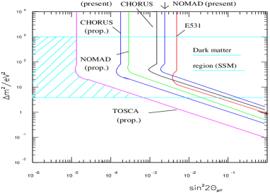
Figure 12: Status and proposed curves for $\nu_{\mu}$ - $\nu_{\tau}$ oscillations. Shaded are the regions expected for an eV-$\nu_{\tau}$ as dark matter candidate according to the see-saw-model, where $\nu_{e}$ - $\nu_{\mu}$ oscillations are used to explain the solar neutrino deficit. Meanwhile the CHORUS and NOMAD exclusion curve moved down to 1.2 $\cdot 10^{-3}$ for large $\Delta m^{2}$ .

Long baseline experiments

Several accelerators and underground laboratories around the world offer the possibility to perform long baseline experiments . This is of special importance to probe the region of atmospheric neutrinos directly.
KEK - Super-Kamiokande : The first of these experiments will be the KEK-E362 experiment (K2K) [153] in Japan sending a neutrino beam from KEK to Super-Kamiokande . The distance is 235 km. A 1 kt near detector, about 1 km away from the beam dump will serve as a reference and measure the neutrino spectrum. The neutrino beam with an average energy of 1 GeV is produced by a 12 GeV proton beam dump. The detection method within Super-Kamiokande will be identical to that of their atmospheric neutrino detection. The beamline should be finished by the end of 1998 and the experiment will start data taking in 1999. In connection with the JHC-project an upgrade of KEK is planned to a 50 GeV proton beam, which could start producing data around 2004 and would make a $\nu_{\tau}$ appearance search possible.
Fermilab - Soudan: A neutrino program is also associated with the new Main Injector at Fermilab. The long baseline project will send a neutrino beam to the Soudan mine about 735 km away from Fermilab. Here the MINOS experiment [154] will be installed. It also consists of a near detector located at Fermilab and a far detector at Soudan. The far detector will be made of 8 kt magnetized Fe toroids in 600 layers with 2.54 cm thickness interrupted by about 32000 m² active detector planes in form of plastic scintillator strips with x and y readout to get the necessary tracking informations. An additional hybrid emulsion detector for $\tau$-appearance is also under consideration. The project could start at the beginning of next century.
CERN - Gran Sasso: A further program considered in Europe are long baseline experiments using a neutrino beam from CERN down to Gran Sasso Laboratory. The distance is 732 km. Several experiments have been proposed for the oscillation search. The first proposal is the ICARUS experiment [155] which will be installed in Gran Sasso anyway for the search of proton decay and solar neutrinos. This liquid Ar TPC can also be used for long baseline searches. A prototype of 600 t is approved for installation which will happen in 1999. A second proposal, the NOE experiment [156], plans to build a giant lead-scintillating fibre detector with a total mass of 4.3 kt. The calorimeter modules will be interleaved with transition radiation detectors with a total of 2.4 kt. The complete detector will have twelve modules, each 8m$\times$8m$\times$5m, and a module for muon identification at the end. A third proposal is the building of a 125 kt water-RICH detector (AQUA-RICH) [157], which could be installed outside the Gran Sasso tunnel. The readout will be done by 3600 HPDs with a diameter of 250 mm and having single photon sensitivity. Finally there exists a proposal for a 750t iron-emulsion sandwich detector (OPERA) [158] which could be installed either at the Fermilab-Soudan or the CERN-Gran Sasso project. It could consist of 92 modules, each would have a dimension orthogonal to the beam of 3$\times$3 m² and would consist out of 30 sandwiches. One sandwich is composed out of 1 mm iron, followed by two 50 $\mu$m emulsion sheets, spaced by 100 $\mu$m. After a gap of 2.5 mm, which could be filled by low density material, two additional emulsion sheets are installed. The $\tau$, produced by CC reaction in the iron, decays in the gap region, and the emulsion sheets are used to verify the kink of the decay.
A project in the very far future could be oscillation experiments involving a $\mu^{+}\mu^{-}$-collider currently under investigation. The created neutrino beam is basically free of $\nu_{\tau}$ and can be precisely determined to be 50 % $\mbox{$\nu_{\mu}$}(\bar{\nu}_{\mu})$ and 50% $\bar{\nu}_{e}$ ($\nu_{e}$) for $\mu^{-}(\mu^{+})$. Because the $\mu^{+}\mu^{-}$-collider would be a high luminosity machine, one even can envisage very long baseline experiments e.g. from Fermilab to Gran Sasso with a distance of 9900 km [159].

5.4 Atmospheric neutrinos

A different source of neutrinos are cosmic ray interactions within the atmosphere. A detailed prediction of the expected flux depends on three main ingredients, namely the cosmic ray spectrum and composition, the geomagnetic cutoff and the neutrino yield of the hadronic interaction in the atmosphere. At lower energies ($E\mbox{$\stackrel{{\scriptstyle<}}{{\sim}}$ }$1 GeV) neutrinos basically result from pion- and muon-decay leading to rough expectations for the fluxes like $\mbox{$\nu_{\mu}$}\sim\mbox{$\bar{\nu}_{\mu}$}\sim 2\mbox{$\nu_{e}$}$ or $\mbox{$\nu_{e}$}/\mbox{$\bar{\nu}_{e}$}\sim\mu^{+}/\mu^{-}$. The ratio $\nu_{e}$ / $\nu_{\mu}$ drops quickly above 1 GeV, because for $E_{\mu}>2.5$ GeV the path length for muons becomes larger than the production height. At even higher energies the main source of $\nu_{e}$ are $K_{e3}$-decays ($K^{0}_{L}\rightarrow\pi e\mbox{$\nu_{e}$}$). Contributions of prompt neutrinos from charm decay are negligible and might become important in the region above 10 TeV [160].

Figure 13: Different classes of observable muons as a function of neutrino energy. The peak corresponding to contained events is reduced by a factor 10 (after [262]).

For neutrinos in the energy range 300 MeV $\stackrel{{\scriptstyle<}}{{\sim}}$ $E_{\nu}$ $\stackrel{{\scriptstyle<}}{{\sim}}$ 3 GeV the energy of the primary typically lies in the region 5 GeV $\stackrel{{\scriptstyle<}}{{\sim}}$ $E_{P}$ $\stackrel{{\scriptstyle<}}{{\sim}}$ 50 GeV. This region of the spectrum is affected by the geomagnetic cutoff, which depends on the gyroradius of the particles, introducing a factor A/Z between nuclei and protons of the same energy. However neutrino production depends on the energy per nucleon E/N. Furthermore the energy range below about 20 GeV is also affected by the 11-year activity cycle of the sun, which is in the maximum phase preventing low energy cosmic rays to penetrate into the inner solar system. Neutrinos in the region well beyond 1 GeV can be detected via horizontal or upward going muons produced by CC reactions. The dominant part is given from events between 10 GeV $<\mbox{$E_{\nu}$}<10^{4}$ GeV. The contribution of primaries with energies larger than $10^{5}$ GeV/nucleon to the upward going muon flux is only about 15 %. Several authors made calculations for the neutrino flux for different detector sites covering the energy region from 100 MeV to $10^{4}$ GeV [161, 162, 163, 164, 165, 166]. The absolute predictions differ by about 30 % due to different assumptions on the cosmic ray spectrum and composition and the description of the hadronic interaction. Absolute atmospheric neutrino spectra in the interval 320 MeV $<E_{\mbox{$\nu_{e}$}}<$ 30 GeV for $\nu_{e}$ and 250 MeV $<E_{\mbox{$\nu_{\mu}$}}<$ 10 TeV are measured by the Frejus-experiment [167]. The observed neutrino event types can be divided by their experimental separation into contained, stopped and throughgoing events (Fig.13). For neutrino oscillation searches it is convenient to use the ratio $\mu$/e or even the double ratio R of experimental values versus Monte Carlo prediction

$$R=\frac{(\mu/e)_{exp}}{(\mu/e)_{MC}}$$ (76)

where $\mu$ denotes muon-like and $e$ electron-like events. Here a large number of systematic effects cancel out. The above mentioned calculations agree for $R$ within 5 % for $E_{\nu}$ between 400 MeV and 1 GeV but show a significant difference in normalisation and spectral shape. This effect can mainly be traced back to different assumptions on the production of low energy pions from 10 - 30 GeV p-Air interactions. This might be improved by the results of the recent NA56 measurements [142]. Furthermore the predictions can be cross-checked with atmospheric muon flux measurements which are closely related [168, 169, 170].
The purest sample to investigate are the contained events corresponding to $E_{\nu}$ $\stackrel{{\scriptstyle<}}{{\sim}}$ 1 GeV. The events are basically due to quasielastic CC and single pion NC reactions [171]. Unfortunately the relevant cross sections for these processes have a relatively large uncertainty in the energy range of interest. By far the highest statistics for the sub-GeV region ($E_{vis}<1.33$ GeV, where $E_{vis}$ is the energy of an electromagnetic shower producing a certain amount of Cerenkov-light) is given by Super-Kamiokande . With a significance of 33 kt$\times$y they accumulated 1158 $\mu$-like and 1231 e-like events in their contained single ring sample [172]. The capability to distinguish e-like and $\mu$-like events in water Cerenkov-detectors was verified at KEK [173]. The momentum spectra are shown in Fig.14. The value obtained with two independent analyses is given by $R=0.61\pm 0.03(stat.)\pm 0.05(sys.)$.

Figure 14: Momentum spectra of Super-Kamiokande sub-GeV sample a) for the e-like events b) for the $\mu$-like events and c) the obtained $R$-ratio. $R$ stays essentially flat over all five bins (from [172]).

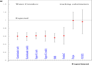
Figure 15: Observed R-values by different experiments . No oscillation corresponds to R=1.

A compilation of experimental results is shown in Table 8 (Fig. 15).

Table 8: Compilation of existing R ratio measurements. The statistics is now clearly dominated by Super-Kamiokande . The no oscillation case corresponds to R = 1.

Experiment	R	stat. significance (kT $\times$ y)
Super-Kamiokande (sub GeV)	$0.63\pm 0.03\pm 0.05$	33.0
Super-Kamiokande (multi GeV)	$0.65\pm 0.05\pm 0.08$	33.0
Soudan2	$0.61\pm 0.15\pm 0.05$	3.2
IMB	$0.54\pm 0.05\pm 0.11$	7.7
Kamiokande (sub GeV)	$0.60^{+0.06}_{-0.05}\pm 0.05$	7.7
Kamiokande (multi GeV)	$0.57^{+0.08}_{-0.07}\pm 0.07$	7.7
Frejus	$1.00\pm 0.15\pm 0.08$	2.0
Nusex	$0.96^{+0.32}_{-0.28}$	0.74

While Frejus and NUSEX are in agreement with expectations, it can be seen that the water Cerenkov detectors and Soudan2 show a significant reduction. Besides looking on the R-ratio for oscillation searches, the zenith angle distribution can be used (Fig.16).

Figure 16: Zenith angle dependence of R for the sub- (left) and multi-GeV (right) sample of Super-Kamiokande . The line in the multi-GeV sample corresponds to $\nu_{\mu}$ - $\nu_{\tau}$ oscillations with $sin^{2}2\theta$ =1 and $\Delta m^{2}$ = $5\cdot 10^{-3}eV^{2}$ (from [172, 174]).

Because the baselines are quite different for downward (L $\approx$ 20 km) and upward going muons (L $\approx 10^{4}$ km), any oscillation effect should show up in a zenith angle dependence. The recent distributions from Super-Kamiokande also for the multi-GeV sample ($E_{vis}>1.33$ GeV), consisting of contained and partially contained events, are shown in Fig. 17 showing an up-down asymmetry which could be explained by neutrino oscillations [174, 175]. To verify this assumption an L/E analysis for fixed $\Delta m^{2}$ , as the one proposed for the LEP-experiments in [176], is done, which shows a characteristic oscillation pattern. From the zenith angle distribution and the momentum spectra it seems evident that there is a deficit in muon-like events, which might be explained by $\mbox{$\nu_{\mu}$}-\mbox{$\nu_{\tau}$}$ or $\mbox{$\nu_{\mu}$}-\nu_{S}$ oscillations. The region allowed by $\mbox{$\nu_{\mu}$}-\mbox{$\nu_{\tau}$}$ oscillations is shown in Fig.18. An independent three flavour analysis results in a best fit value of $\Delta m^{2}$ $\approx 7\cdot 10^{-3}eV^{2}$ for maximal mixing [177]. Additionally the CHOOZ-result excludes all Kamiokande data to be due to $\mbox{$\nu_{\mu}$}-\mbox{$\nu_{e}$}$ oscillations and are shown for comparison in Fig.18 as well. Moreover in a recent analysis of all atmospheric data including the earth matter effect (see chapter 6.3.2), the CHOOZ-result rules out the $\nu_{\mu}$ - $\nu_{e}$ solution for Super-K at 90 % CL [178]. Furthermore different oscillation channels might be distinguished by a detailed investigation of up-down asymmetries [179] or by measuring the NC/CC ratio [180].

Figure 17: Zenith angle distribution of electron- (left) and muon like (right) events for the sub- and multi GeV sample of Super-Kamiokande . The bars correspond to MC expection without neutrino oscillations and are reflecting the statistical uncertainty. The $\pm$ 20 % normalisation uncertainty is not shown. The normalisation is adjusted to the upward going events. The dotted curve corresponds to a $\nu_{\mu}$ -$\nu_{\tau}$ oscillation scenario with $sin^{2}2\theta$ = 1 and $\Delta m^{2}$ = $5\cdot 10^{-3}eV^{2}$. A clear $\mu$-deficit coming from below can be seen. The ratio R obtained from the histograms is shown in Fig. 16 (from [174]).

Figure 18: a) $\nu_{\mu}$ - $\nu_{\tau}$ allowed region of Super-Kamiokande analysis of zenith angle distribution (from [175]). b) $\nu_{e}$ - $\nu_{\mu}$ exclusion plot as given by reactor experiments especially CHOOZ. This excludes any interpretation of atmospheric neutrino data as observed by Kamiokande by oscillations in this channel (from [130]).

Neutrino events at higher energies are detected via their CC reactions producing upward going muons . The effective detector area can be increased because of the muon range allowing $\nu_{\mu}$ CC in the surrounding rock (see chapter 7.2.2). The corresponding muon flux of the used horizontal and upward going muons has to be compared with absolute predictions. One also has to take care of the angular dependent acceptance of the detector. Here the main uncertainty for the neutrino flux stems from kaon production and the knowledge of the involved structure functions. The behaviour of low-energy cross sections is dicussed in [171]. Also here the models can be adjusted to recent muon flux measurements in the atmosphere [168] even though one has to take into account that for E$>$100 GeV relatively more neutrinos are produced by kaon-decays while the muon-flux is still given dominantly by pion-decay. The observations of upward going muons are compiled in Fig.19. A zenith angle distribution from upward going muons as measured with Super-Kamiokande is shown in Fig. 19. Two independent ways of verifying the oscillation solution are the ratio of stopped/throughgoing muons and the shape of the zenith angle distribution [181]. Both were done by Super-Kamiokande and support their oscillation evidence [174].

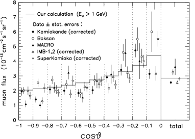
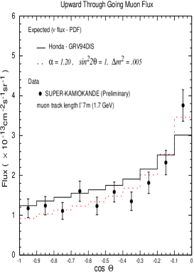
Figure 19: Zenith angle distribution of upward going muons compiled by Fogli et al. [182] as of Aug. 1997 (left). The up-to-date spectrum as observed by Super-Kamiokande is shown on the right. The line corresponds to the flux predictions of Honda et al. [183] and using the GRV 94 DIS structure functions [184]. An oscillation scenario with $sin^{2}2\theta$ = 1 and $\Delta m^{2}$ = $5\cdot 10^{-3}eV^{2}$ including a factor $\alpha=1.2$ in the normalisation is shown as a dotted curve (from [175]).

6 Solar neutrinos

The closest astronomical neutrino source is the sun. The investigation and understanding of the sun as a typical main sequence star is of outstanding importance for an understanding of stellar evolution. Stars are producing their energy via nuclear reactions. The hydrogen burning is done in two ways as shown in Fig.20, the pp-chain and the CNO-chain. The net result is the same giving

$$4p\rightarrow\mbox{${}^{4}He$ }+2\mbox{$\nu_{e}$}+26.73MeV$$ (77)

The prediction of the expected neutrino flux depends on detailed calculations of the solar structure resulting in temperature, pressure and density profiles and the knowledge of nuclear cross sections for determining the energy generation. Once the flux is in hand, it is still a matter of detecting this low-energy neutrinos typically below 15 MeV with the main component below 500 keV. The principle methods are radiochemical detectors using inverse $\beta$-decay and real-time experiments looking for neutrino-electron scattering. Because of the low cross-sections involved, it is convenient to introduce a new unit for the expected event rates in radiochemical detectors called SNU (solar neutrino unit) given by

$$1SNU=10^{-36}\quad\mbox{captures per target atom per second}$$ (78)

The fundamental equations and ingredients of standard solar models are discussed first. For more detailed reviews see [185, 186, 187].

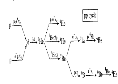
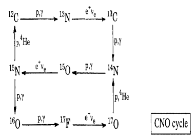
Figure 20: Energy generation in the sun via the pp und CNO cycles.

6.1 Standard solar models (SSM)

The sun as a main sequence star is producing its energy by hydrogen fusion and its stability is ruled by thermal and hydrodynamic equilibrium. Modelling of the sun as well as the prediction of the expected neutrino flux requires the basic equations of stellar evolution:
Mass conservation

$$\frac{dM(r)}{dr}=4\pi r^{2}\rho(r)$$ (79)

where $M(r)$ denotes the mass within a sphere of radius $r$.
Hydrostatic equilibrium (gravity is balanced by gas and radiation pressure)

$$\frac{dp(r)}{dr}=-\frac{GM(r)}{r^{2}}\rho(r)$$ (80)

Energy balance, meaning the observed luminosity L is generated by an energy generation rate $\epsilon$

$$\frac{dL(r)}{dr}=4\pi r^{2}\rho(r)\epsilon$$ (81)

Energy transport dominantly by radiation and convection which is given in the radiation case by

$$\frac{dT(r)}{dr}=-\frac{3}{64\pi\sigma}\frac{\kappa\rho(r)L(r)}{r^{2}T^{3}}$$ (82)

with $\sigma$ as the Stefan-Boltzman constant and $\kappa$ as absorption coefficient. These equations are governed by additional three equations of state for the pressure $p$, the absorption coefficient $\kappa$ and the energy generation rate $\epsilon$:

$$p=p(\rho,T,X),\quad\kappa=\kappa(\rho,T,X),\quad\epsilon=\epsilon(\rho,T,X)$$ (83)

where $X$ denotes the chemical composition. The Russell-Vogt theorem then assures, that for a given $M$ and $X$ an unique equilibrium configuration will evolve, resulting in certain radial pressure, temperature and density profiles. Under these assumptions, solar models can be calculated as an evolutionary sequence from an initial chemical composition. The boundary conditions are that the model has to reproduce the age, luminosity, surface temperature and mass of the present sun. The two typical adjustable parameters are the ${}^{4}He$ abundance and the relation of the convective mixing length to the pressure scale height. This task has been done by several groups [187, 188, 189, 190, 191, 192, 193]. Nevertheless there remain sources of uncertainties. Some will be discussed in a little more detail.

6.1.1 Diffusion

Several experimental evidences strongly suggest a significant mixing and gravitational settling of He and the heavier elements in the sun. The long standing problem of ${}^{7}Li$ - depletion in the solar photosphere can be explained if ${}^{7}Li$ is destroyed by nuclear burning processes, which on the other hand requires temperatures of about 2.6 $\cdot 10^{6}$ K. Such temperatures exist nowhere at the base of the convection zone, therefore ${}^{7}Li$ has to be brought to the inner regions. Also the measured sound speed profiles in the solar interior obtained by helioseismological data can be better reproduced by including diffusion processes. Therefore these effects were included in the latest solar models.

6.1.2 Initial composition

The chemical abundances of the heavier elements (larger than helium) is an important ingredient for solar modelling. Their abundances influence the radiative opacity and therefore the temperature profile within the sun. Under the assumption of a homogeneous sun, it is assumed that the element abundance in the solar photosphere still corresponds to the initial values. The relative abundances of the heavy elements are best determined in certain kind of meteorites, the type I carbonaceous chondrites, which can be linked and found in good agreement with the photospheric abundances [194, 195]. Abundances of C,N and O are taken from photospheric values, the ${}^{4}He$ abundance cannot be measured and is used as an adjustable parameter.

6.1.3 Opacity and equation of state

The opacity or Rosseland mean absorption coefficient $\kappa$ is defined as a harmonic mean integrated over all frequencies $\nu$

$$\frac{1}{\kappa}=\frac{\int_{0}^{\infty}\frac{1}{\kappa_{\nu}}\frac{dB_{\nu}}{dT}d\nu}{\int_{0}^{\infty}\frac{dB_{\nu}}{dT}d\nu}$$ (84)

where $B_{\nu}$ denotes a Planck-spectrum. The implication is that more energy is transported at frequencies at which the material is more transparent and at which the radiation field is more temperature dependent. The calculation of the Rosseland mean requires a knowledge of all involved absorption and scattering cross sections of photons on atoms, ions and electrons. The calculation includes bound-bound (absorption), bound-free (photoionization), free-free (inverse bremsstrahlung) transitions and Thomson-scattering. Corrections for electrostatic interactions of the ions with electrons and for stimulated emissions have to be taken into acount. The number densities $n_{i}$ of the absorbers can be extracted from the Boltzmann and Saha equations. The radiative opacity per unit mass can then be expressed as (with the substitution u= $h\nu/kT$)

$$\frac{1}{\kappa}=\rho\int_{0}^{\infty}\frac{15u^{4}e^{u}/4\pi^{4}(e^{u}-1)^{2}}{(1-e^{u})\sum_{i}\sigma_{i}n_{i}+\sigma_{s}n_{e}}du$$ (85)

where $\sigma_{s}$ denotes the Thomson scattering cross section.
The most comprehensive compilation of opacities is given by the Livermore group (OPAL) [196, 197]. It includes data of 19 elements in a wide range of temperature, density and composition. The main contribution to the opacity in the centre of the sun is given by inverse bremsstrahlung with a few per cent contribution of Thomson scattering. A detailed study on opacity effects on the solar interior can be found in Tripathy et al. [198].
A further ingredient for solar model calculations is the equation of state, meaning the density as a function of $p$ and $T$ or as widely used in the calculations, the pressure expressed as a function of density and temperature. Except for the solar atmosphere, the gas pressure outweighs the radiation pressure anywhere in the sun. The gas pressure is given by the perfect gas law, where the mean molecular weight $\mu$ must be determined by the corresponding element abundances. The different degrees of ionisation can be determined using the Saha equations. An equation of state in the solar interior has to consider plasma effects (normally via Debye-Hückel treatment) and the partial electron degeneracy deep in the solar core. The latest equation of state is given by Rogers et al. [199].

6.1.4 Nuclear reaction rates

A detailed prediction of the solar structure and the corresponding neutrino flux relies on the nuclear reaction rates [200, 201]. Their precise knowledge determines the branching in the complex network of reactions and the yields of all isotopes. In contrast to typical energies in the solar interior, which are in the keV region (Gamow-region), laboratory measurements are normally at about MeV and one has to extrapolate down. Because the cross section for non-resonant charged particle interactions is steeply falling, it is usually parametrized as

$$\sigma(E)=\frac{S(E)}{E}exp(-2\pi\eta)$$ (86)

where the Sommerfeld-parameter $\eta$ is given by $\eta=Z_{1}Z_{2}e^{2}/\hbar v$. In cases of no resonances, the nuclear or astrophysical S-factor S(E) should show a rather smooth behaviour. It is therefore typically the S-factor which is extrapolated down to solar energies. Since the energy of the Gamow-Peak is temperature dependent, S(E) is for ease of computation expanded in a Taylor series with respect to energy

$$S(E)=S(0)+\dot{S}(0)E+\frac{1}{2}\ddot{S}(0)E^{2}+...$$ (87)

where $S(0),\dot{S}(0)$ etc. are obtained by a fit to the experimental data. A compilation of S(0) values for all relevant reactions of the pp-cycle can be found in Table 9. Because such extrapolations contain some uncertainties, the idea is to measure the cross section directly in the relevant energy range. To reach this goal, several additional requirements have to be fulfilled, e.g. going underground. In a first step this is done by the LUNA collaboration building a 50 kV accelerator at Gran Sasso Laboratory to investigate the ${}^{3}He$ (${}^{3}He$ ,2p)${}^{4}He$ reaction as the final step in the ppI-chain [202]. As can be seen in Fig. 21, the experimental data exceed the theoretical expectation of bare nuclei which is due to a still restricted knowledge of screening effects.

Figure 21: Cross section for the ${}^{3}He$ (${}^{3}He$ ,2p)${}^{4}He$ at low energies as obtained with the LUNA experiment . For the first time data points directly in the Gamow peak are experimentally obtained (from [202]).

Further activities will include an upgrade to a 200 kV and even 2 MV accelerator making the additional measurements of the ${}^{7}Be$ (p,$\gamma$)${}^{8}B$ and ${}^{14}N(p,\gamma$)${}^{15}O$ cross sections possible. New measurements for the ${}^{7}Be$ (p,$\gamma$)${}^{8}B$ cross section at cms energies between 350 and 1400 keV exist [203]. Earlier measurements of Kavanagh et al. [204] and Fillipone et al. [205] showed a 30 % difference in the absolute value of S(E) in this region. The new measurement seems to support the lower S(E) values of [205]. A further proposal to investigate this important cross-section exists by using ISOLDE at CERN [206].

Table 9: Compilation of S(0) values relevant for the pp-process. For most reactions the 1$\sigma$ error is given.

reaction	S(0) (keV $\cdot$b)
pp$\rightarrow de^{+}\nu$	$4.00(1\pm 0.007^{+0.020}_{-0.011})\cdot 10^{-22}$
d(p,$\gamma$)${}^{3}He$	0.25 $\cdot 10^{-3}$
${}^{3}He$ (${}^{3}He$ ,2p)${}^{4}He$	5400 $\pm$ 400
${}^{3}He$ (p,$e^{+}$ $\nu_{e}$ )${}^{4}He$	2.3 $\cdot 10^{-20}$
${}^{3}He$ ($\alpha,\gamma$)${}^{7}Be$	0.53 $\pm$ 0.05
${}^{7}Be$ (p,$\gamma$)${}^{8}B$	0.019${}^{+0.004}_{-0.002}$

6.1.5 Neutrino flux predictions

Several groups are working on the detailed modelling of the sun in order to predict accurately the solar neutrino flux and to reproduce the sound speed profile measured with helioseismology. A comparison of the different predicted neutrino fluxes at the position of the earth is given in Table 10 and Fig.22.

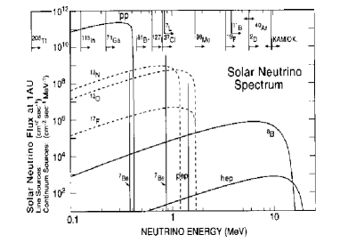
Figure 22: Predicted solar neutrino spectrum including thresholds for various running and planned experiments (with kind permission of T. Kirsten).

Table 10: Flux predictions from four different solar model calculations.

Flux ($cm^{-2}s^{-1}$ )	BP95 [187]	RVCD [191]	CDFLR [193]	DS96 [192]
${\phi}_{\nu}(pp)~{}[{10}^{10}\mbox{$cm^{-2}s^{-1}$ }]$	5.91	5.94	5.99	6.10
${\phi}_{\nu}(pep)~{}[{10}^{8}$$cm^{-2}s^{-1}$ ]	1.40	1.38	1.40	1.43
${\phi}_{\nu}(^{7}{Be})~{}[{10}^{9}$$cm^{-2}s^{-1}$ ]	5.15	4.80	4.49	3.71
${\phi}_{\nu}(^{8}{B})~{}[{10}^{6}$$cm^{-2}s^{-1}$ ]	6.62	6.33	5.16	2.49
${\phi}_{\nu}(^{13}{N})~{}[{10}^{8}$$cm^{-2}s^{-1}$ ]	6.18	5.59	5.30	3.82
${\phi}_{\nu}(^{15}{O})~{}[{10}^{8}$$cm^{-2}s^{-1}$ ]	5.45	4.81	4.50	3.74

6.2 Solar neutrino experiments

At present results of five neutrino experiments are available, namely the chlorine-experiment, the two gallium experiments GALLEX and SAGE and the only real-time experiment Kamiokande and its follow-up Super-Kamiokande. The discussion follows the historical ordering starting with the chlorine-experiment.

6.2.1 The chlorine-experiment

The origin of neutrino astrophysics is the chlorine solar neutrino experiment by R. Davis in the Homestake mine in South Dakota [207, 208]. The detection reaction is

$$^{37}Cl+\nu_{e}\rightarrow^{37}Ar+e^{-}$$ (88)

with a threshold of 814 keV. Therefore it is basically sensitive to ${}^{8}B$ and ${}^{7}Be$ neutrinos with small contributions due to pep, ${}^{13}N$ and ${}^{15}O$ neutrinos. All, except the ${}^{8}B$ neutrinos , lead only to the ground state of ${}^{37}Ar$ whereas ${}^{8}B$ is also populating excited states including the isotopic analogue state. The cross section for the reaction (88) averaged over the ${}^{8}B$ spectrum has been measured recently to be [209, 210]

$$1.14\pm 0.11\cdot 10^{-42}cm^{2}$$ (89)

The predicted SNU-rate for the experiment due to different flux contributions is given in Table 11.

Table 11: Contributions (in SNU) of the different flux components of solar neutrinos to the signal in different radiochemical detector materials of running or planned experiments . The fluxes of BP95 are used.

Source	${}^{37}Cl$	${}^{71}Ga$	${}^{127}I$	${}^{7}Li$	${}^{131}Xe$
pp	0	69.7	0	0	9.7
pep	0.22	3.0	1.85	9.17	1.6
${}^{7}Be$	1.24	37.7	13.0	9.78	17.8
${}^{8}B$	7.36	16.1	18.4	25.8	12.7
${}^{13}N$	0.11	3.8	0.73	2.62	1.6
${}^{15}O$	0.37	6.3	2.43	13.4	1.8
Sum	9.3	136.6	36.5	60.8	45.2

The production of one ${}^{37}Ar$ atom/day corresponds to 5.35 SNU. The experiment consists of 615 t tetrachloroethylene (C₂Cl₄) under a shielding of about 4000 mwe. The natural abundance of ${}^{37}Cl$ is 24 % resulting in 2.2 $\cdot 10^{30}$ target atoms. An extraction of the produced ${}^{37}Ar$ happens roughly every two months, and the extraction efficiency is controlled by adding a small amount of isotopical pure inert ${}^{36}Ar$ or ${}^{38}Ar$ . To do this, helium is flushed through the tank taking the volatile argon out of the solution and allowing the collection of the argon in a cooled charcoal trap. After purification, the argon is filled with the counting gas P10 into specially developed low-level miniaturized proportional counters. The detection reaction uses the EC of ${}^{37}Ar$

$$e^{-}+\mbox{${}^{37}Ar$ }\rightarrow\mbox{${}^{37}Cl$ }+\nu_{e}$$ (90)

with a half-life of 35 days and focuses on observing the 2.82 keV Auger electrons. To discriminate further against background energy and pulse rise time information are used and the counters are plugged into a special low-level shielding. The average measured value using 108 runs after starting the experiment in 1970 is given by [211]

$$2.56\pm 0.16(stat.)\pm 0.15(sys.)SNU$$ (91)

whereas the single runs can be seen in Fig. 23. The theoretical expectations are 9.3 $\pm$ 1.4 SNU [187], 4.1 $\pm$ 1.2 SNU [192] and 6.4 $\pm$ 1.4 SNU [190]. This discrepancy is the origin of the solar neutrino problem.

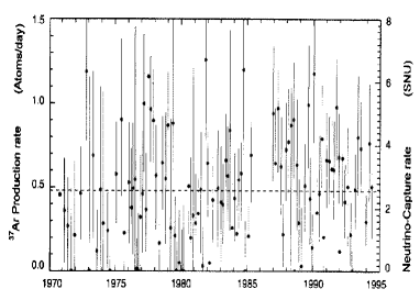
Figure 23: SNU-rate as function of time for the Cl-experiment (from [211]).

6.2.2 Real time water Cerenkov detectors

The only real time solar neutrino experiments are Super-Kamiokande and its precessor Kamiokande. The detection principle is the Cerenkov light produced in neutrino-electron scattering within the water. Energy and directional information are reconstructed from the corresponding number and timing of the hit photomultipliers. The scattering angle of the struck electron is related with the incident neutrino energy as

$$cos\theta_{e}=\frac{1+\frac{m_{e}}{E_{\nu}}}{1+\frac{2m_{e}}{T_{e}}}$$ (92)

where $T_{e}$ denotes the kinetic energy of the recoil electron. The directional information is shown in Fig.24. While Kamiokande consisted out of 3000t of water using only 680 tons as fiducial volume, Super-Kamiokande consists of 50000 t using 22.5 kt as fiducial volume. The detector threshold is 6.5 MeV for Super-Kamiokande (in the late stage of Kamiokande it was at 7.5 MeV) making these detectors only sensitive to ${}^{8}B$ neutrinos. The measured fluxes are [212]

$$\Phi(\mbox{${}^{8}B$ }) = 2.80\pm 0.19\pm 0.33\cdot 10^{6}\mbox{$cm^{-2}s^{-1}$ }\quad\mbox{Kamiokande (final)}$$ (93)

$$\Phi(\mbox{${}^{8}B$ }) = 2.44\pm 0.05(stat.)^{+0.09}_{-0.07}(sys.)\cdot 10^{6}\mbox{$cm^{-2}s^{-1}$ }\quad\mbox{Super-Kamiokande }$$ (94)

where the theoretical expectations are $6.62\cdot 10^{6}\mbox{$cm^{-2}s^{-1}$ }$ (BP), $4.52\cdot 10^{6}\mbox{$cm^{-2}s^{-1}$ }$ (TCL) and $2.49\cdot 10^{6}\mbox{$cm^{-2}s^{-1}$ }$ (DS). The ratio of measured to expected electron recoil spectrum is given in Fig. 25. Super-Kamiokande recently implemented a low energy trigger with a threshold of 4.5 MeV.

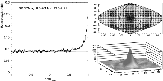
Figure 24: Angular distribution of observed recoil electrons in Super-Kamiokande . Clearly visible is an increase in direction of the sun (cos $\theta$ =1). The double angle plots (right) with the sun at (0,0) show clearly that the neutrinos are coming from the sun (from [213]).

Figure 25: Energy spectrum of ${}^{8}B$ neutrinos as observed by Super-Kamiokande divided by the solar model of [184]. The solid line corresponds to a fit with a SMA solution (from [212]).

6.2.3 The gallium experiments

The only experiments which are able to measure the pp- neutrinos directly are GALLEX and SAGE, using ${}^{71}Ga$ as target material. The underlying reaction is

$${}^{71}Ga+\nu_{e}\rightarrow^{71}Ge+e^{-}$$ (95)

with a threshold of 233 keV. The main difference between the two experiments lies in the chemical state of the gallium and therefore also in the extraction of the produced ${}^{71}Ge$ . While GALLEX is using 30 t of gallium in form of a 110 t GaCl₃ solution, SAGE is using about 57 tons of metallic gallium. After extraction, ${}^{71}Ge$ is converted into GeH₄ and filled together with Xe into special miniaturised proportional counters. The detection relies on the Auger-electrons and X-rays from K and L-capture in the ${}^{71}Ge$ decay producing two lines at 10.37 keV and 1.2 keV. As in the chlorine-experiment, besides the energy information also pulse rise time analysis is used and the counting is done inside a special low-level shielding. Both experiments for the first time checked their overall efficiency by using MCi ${}^{51}Cr$ sources. The present results are [214, 215]

$$76.4\pm 6.3(stat.)^{+4.5}_{-4.9}(sys.)\quad SNU\quad\mbox{GALLEX }$$ (96)

$$66.6^{+6.8}_{-7.1}(stat.)^{+3.8}_{-4.0}(sys.)\quad SNU\quad\mbox{SAGE}$$ (97)

with theoretical predictions of $137^{+8}_{-7}$ SNU [216], $123\pm 8$ [190] and $115\pm 6$ SNU [192]. Clearly the experiments are far off. The individual runs for GALLEX are shown in Fig. 26.

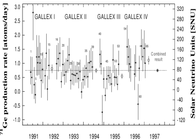
Figure 26: SNU rate as a function of time for the GALLEX experiment (from [215]).

6.3 Solutions to the solar neutrino problem

The observed results split the solar neutrino problem into three. The first and original one is that the measured rate in the chlorine - experiment, dominated by ${}^{8}B$ neutrinos , is less than the SSM prediction. This problem might be explained as an astrophysical solution by reducing the ${}^{8}B$ - flux by a temperature decrease in the solar core or by the involved uncertainties in the nuclear cross sections. On the other hand Super-Kamiokande measures the ${}^{8}B$ - flux and taking this value as a fact, the contribution of the ${}^{8}B$ neutrinos to the chlorine signal already exceeds the experimental value. This is independent of any solar model. There is no astrophysical scenario which could distort the ${}^{8}B$ beta spectrum in such a way that both experiments are in agreement. Any possible deviation is shown to be at maximum at the 10^-5 level [217]. There is almost no room for the ${}^{7}Be$ neutrinos , but ${}^{8}B$ is produced from ${}^{7}Be$ . The third problem is, that the gallium experiments do not allow any significant contribution beside the expected pp-value. Also here there is almost no room for the ${}^{7}Be$ neutrinos contributing more than 30 SNU in the SSM. A fit to all available data, independent of a solar model, is given by Hata et al. [218] and shown in Fig. 27. The best fit values achieved for the fluxes are $\Phi(\mbox{${}^{7}Be$ })/\Phi(\mbox{${}^{7}Be$ })_{SSM}=-0.6\pm 0.4$ and $\Phi(\mbox{${}^{8}B$ })/\Phi(\mbox{${}^{8}B$ })_{SSM}=0.4\pm 0.5$. Restricting the fluxes to physical regions ($\Phi>0$) changes the result to $\Phi(\mbox{${}^{7}Be$ })/\Phi(\mbox{${}^{7}Be$ })_{SSM}<0.1$ and $\Phi(\mbox{${}^{8}B$ })/\Phi(\mbox{${}^{8}B$ })_{SSM}=0.38\pm 0.05$ using the solar model of Bahcall and Pinnsoneault [187].

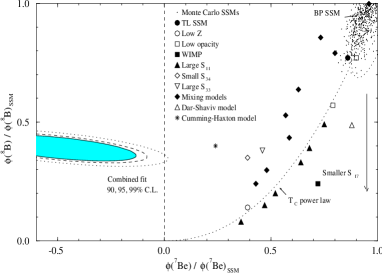
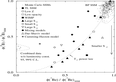
Figure 27: Constraints from the Cl,Ga and Cerenkov-experiments in comparison with several flux predictions. In the upper right corner are the solar models from Bahcall and Pinnsoneault [187], the dashed curve corresponds to a power law behaviour of the solar core temperature and the other mentioned solar models are explained in Hata and Langacker [219]. Reducing the $S_{17}$ factor leads to an evolution in the direction of the arrow. The fit to the experimental data results in negative values for the ${}^{7}Be$ flux (grey area). On the right side no luminosity constraint is implemented (from [218]).

6.3.1 Astrophysical and nuclear solutions

Typical astrophysical solutions try in some way to reduce the central temperature in the sun to account for less high energetic neutrinos . For an overview see [186]. Because of the strong temperature dependence of the ${}^{8}B$ -flux ($\propto T^{18}$), a reduction to 96 % of the SSM of BP value could explain the Super-Kamiokande data. However the ratio $\Phi(\mbox{${}^{7}Be$ })/\Phi(\mbox{${}^{8}B$ })\propto T^{-10}$ increases in contrast to experiments which basically imply no ${}^{7}Be$ neutrinos at all. This is the main reason why neutrino solutions are preferred. A way to circumvent this naive T dependence is given by Cumming et al. [220] assuming a slow mixing of the solar core on timescales characteristic of ${}^{3}He$ equilibrium. The result is a remarkably different out-of equilibrium ${}^{3}He$ - profile in the solar core leading to two consequences: First of all, more helium is produced via the ${}^{3}He$ (${}^{3}He$ ,2p)${}^{4}He$ chain reducing the ${}^{7}Be$ and ${}^{8}B$ neutrino flux and secondly, the short-living ${}^{7}Be$ is produced at higher temperature favouring the ${}^{7}Be$ (p,$\gamma$)${}^{8}B$ reaction with respect to ${}^{7}Be$ (e,$\nu_{e}$)${}^{7}Li$ . The combined effect is a somewhat reduced ${}^{8}B$ flux and a significantly reduced ${}^{7}Be$ flux.
All the models experience significant constraints from helioseismological data. The agreement between the measured and calculated sound speed profiles are in good agreement even in the solar interior (Fig. 28) [221]. In the region 0.2 $<r/R_{\odot}<$ 0.65 the deviation from expectation is less than 0.5 % and even in the solar core it seems to be less than 4 %.

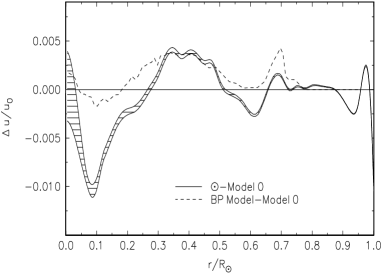
Figure 28: Isothermal sound speed ($u=p/\rho$) profile compared with the reference model of [222] and the standard solar model of [187]. Shown is the deviation of sound speed $\Delta u$ from the calculated value (from [222]).

6.3.2 Neutrino oscillations in matter

An elegant solution to the solar neutrino problem are neutrino oscillations either in vacuum or in matter (MSW-effect). The latter offers the chance to suppress the neutrinos of intermediate energies completely, but leaving the low-energy neutrinos untouched and the high energy neutrinos only partly suppressed. While in solar matter $\nu_{e}$ can interact with electrons via charged and neutral currents, other neutrino flavours only have neutral current interactions. This leads to different forward scattering amplitudes making the mass eigenstates within the sun a function of the electron density. For the oscillation amplitude, a resonance behaviour occurs, allowing maximal mixing even if the vacuum mixing angle is small [223, 224]. The resonance occurs at an electron density $N_{e}$ of

$$N_{e}=\frac{\mbox{$\Delta m^{2}$}cos2\theta}{2\sqrt{2}G_{F}E}$$ (98)

In the adiabatic limit, where the electron density along the trajectory of the neutrino changes slowly enough, a full conversion is achieved, while in the non-adiabatic limit there is a certain transition probability. In case of a linear change in electron density the probability is given by the Landau-Zener probability

$$P(E)=exp(-\frac{\pi\mbox{$\Delta m^{2}$}\mbox{$sin^{2}2\theta$}R_{S}}{E})$$ (99)

with $R_{S}=6.6\cdot 10^{9}$ m. Because the running experiments have different energy thresholds, different contours in the $\Delta m^{2}$ - $sin^{2}2\theta$ plane arise, which overlap only in small regions. Careful statistical analyses have been done by several authors [218, 225, 226, 227]. The preferred solutions are a non-adiabatic or small angle solution (SMA) at $\Delta m^{2}$ $\approx 5\cdot 10^{-6}eV^{2}$ and $sin^{2}2\theta$ $\approx$ 0.008 and a large angle solution (LMA) at $\Delta m^{2}$ $\approx 1.6\cdot 10^{-5}eV^{2}$ and $sin^{2}2\theta$ $\approx$ 0.6 (Fig. 29).

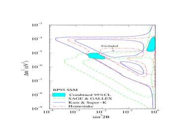
Figure 29: MSW-solutions. The excluded region is given by the non-observation of any day-night effect. The two islands (grey) are the allowed parameters in agreement with all experimental data (from [218]). Also shown are the allowed contours for the single experiments.

Also vacuum oscillations (VAC) are not ruled out [228], giving parameters of $\Delta m^{2}$ $\approx 6\cdot 10^{-11}eV^{2}$ and $sin^{2}2\theta$ $\approx$ 0.9 (Fig. 30). A hybrid solution of vacuum oscillations and MSW-effect seems possible in a three flavour scenario [229]. The upcoming SNO detector will be able to distinguish between all the different solutions. By looking for the electron recoil spectrum as well as the ratio of charged currrent/ neutral current reactions, they should in principle be able to distinguish the solutions with a high confidence level. Also the upcoming radiochemical detectors with their different energy thresholds provide further rejection power between the different solutions.

Figure 30: $\Delta m^{2}$ versus $sin^{2}2\theta$ plot if vacuum oscillations are the explanation for the solar neutrino deficit (from [230]).

The earth can regenerate some of the neutrinos for certain parameter values. By looking for the resulting day(D)-night(N) effect, Super-Kamiokande gives a value of

$$\frac{N-D}{N+D}\times 100=-2.3\pm 2.0(stat.)\pm 1.4(sys.)$$ (100)

showing no hints for such an effect and excluding certain parameter regions in Fig. 29. Because of the long exposure time of the radiochemical experiments, they are not able to search for this effect. Including a second flux independent quantity $\Delta\langle T\rangle/\langle T\rangle$, the deviation of the average measured kinetic energy of the electrons from the standard value, Fogli et al. [230] obtain from the binned spectrum of Super-Kamiokande

$$\Delta\langle T\rangle/\langle T\rangle\times 100=0.95\pm 0.73\quad(1\sigma\quad total)$$ (101)

resulting in a small preference for the SMA-solution (Fig.31).

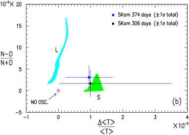
Figure 31: Day-night effect versus the deviation of the electron recoil spectrum. By an accurate measurement of these two flux-independent quantities it seems possible to distinguish the large (L) and small (S) MSW solution. The no oscillation scenario is marked as a star (from [230]).

6.3.3 Neutrino magnetic moments in matter

A similar resonance behaviour can also occur if the solar neutrino problem is solved by a neutrino magnetic moment. The pure spin-flavour precession $\nu_{eL}\rightarrow\nu_{eR}$ in the solar magnetic field cannot explain the data because it results in an energy independent suppression. By allowing spin-flavour transitions like $\nu_{eL}\rightarrow\bar{\nu}_{\mu R}$ it has been shown that a resonance behaviour can occur [231]. The transition probability can be written as [232]

$$P(\nu_{eL}\rightarrow{\bar{\nu}}_{\mu R};r)=\frac{(2\mu B_{\perp})^{2}}{(\mbox{$\Delta m^{2}$}/2E-\sqrt{2}G_{F}N_{eff})^{2}+(2\mu B_{\perp})^{2}}sin^{2}(\frac{1}{2}\sqrt{D}r)$$ (102)

where $D$ is the denominator of the pre-sine factor and $N_{eff}$ is given by $N_{e}-N_{n}/2$ (Dirac) and $N_{e}-N_{n}$ (Majorana) respectively. The most general case is the occurence of two resonances (Fig. 32).

Figure 32: Two resonances can occur for neutrinos coming from the solar interior. First they experience the RSFP resonance and afterwards, if the conversion is not complete, they go through the MSW resonance.

By transversing the sun, neutrinos first undergo the spin-flavour precession and afterwards the MSW-resonance. Depending on the involved $\Delta m^{2}$ and E, the predicted conversion probability can be quite complicated and detailed predictions for the experiments depend on the chosen parameters. It is interesting to note, that in case of adiabacity in the resonant spin-flavour precession scenario a MSW resonance never will occur. Assuming a maximal magnetic field within the sun between 25 -50 kG and a magnetic moment of $\mu_{\nu}$ = $10^{-11}$ $\mu_{B}$ the observed data can be explained if $\Delta m^{2}$ is within a region of $4\cdot 10^{-9}-2\cdot 10^{-8}eV^{2}$. In case both mechanisms are at work the $\Delta m^{2}$ - region is shifted to $10^{-7}-10^{-8}eV^{2}$ and $sin^{2}2\theta$ $<$ 0.25 by allowing a maximal magnetic field between 15-30 kG. Support for this scenario could come from the detection of solar $\bar{\nu}_{e}$ which can be produced via $\nu_{eL}\rightarrow\bar{\nu}_{\mu R}\rightarrow\bar{\nu}_{eR}$. A detailed discussion can be found in [232].

6.4 Future solar neutrino experiments

From the discussion in the last section it seems obvious that the investigation of the ${}^{7}Be$ region needs special attention. At present several experiments are under construction of which some should be able to investigate this region as well as finally solve the problem.

6.4.1 Sudbury Neutrino Observatory

The next real-time solar neutrino experiment which will be online is the Sudbury Neutrino Observatory (SNO). This detector will use 1000 t of D₂O and is installed in the Creighton mine near Sudbury, Ontario. The big advantage of this experiment is a model independent test of the oscillation hypothesis by using weak neutral and charged currents. The detection reactions are

$$\nu_{e}+d\rightarrow e^{-}+p+p$$ (103)

$$\nu+d\rightarrow\nu+p+n$$ (104)

$$\nu+e\rightarrow\nu+e$$ (105)

While the first reaction is flavour sensitive, the second is not. To detect the neutron in the second reaction, two strategies are envisaged: Cl will be added to the heavy water, to use the ${}^{35}Cl(n,\gamma)^{36}Cl$ process and/or a set of He-filled proportional counters will be deployed. The threshold will be around 5-6 MeV and start of measuring is expected in 1998. Beside the NC/CC ratio, the measured electron recoil spectrum of the ${}^{8}B$ neutrinos will provide strong discrimination power among the different scenarios (Fig.33).

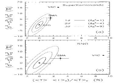
Figure 33: Statistical power of Super-Kamiokande and SNO to distinguish between the different solutions of the solar neutrino problem. Shown are the moments of the electron sprectrum (for details see [225]). The SMA can be checked at the 3$\sigma$ level, the error bars correspond to the experimentally allowed MSW-region (with kind permission of J.N. Bahcall).

6.4.2 BOREXINO

An experiment especially designed to explore the intermediate region containing the ${}^{7}Be$ line at 862 keV is BOREXINO. It will use 300 t of scintillator. The detection relies on neutrino-electron scattering and the detector will be sensitive to neutrino energies larger than 450 keV. Of special importance is the produced ”Compton-Plateau” from the 862 keV line with an expected event rate of 50 per day according to the SSM or about 10 per day in case of the MSW-effect. The detector is extremely sensitive to impurities requiring a background level of $10^{-16}$ g(U,Th)/g. The ability to achieve such low background levels could be demonstrated in a smaller pilot experiment (CTF). BOREXINO is currently installed in the Gran Sasso Laboratory. Data taking should start around 2001.

6.4.3 ICARUS

The ICARUS experiment plans to use in full scale about 3000t LAr in form of a TPC for solar neutrino detection. The technique offers precise tracking with high resolution dE/dx measurement, full event reconstruction in a bubble chamber-like quality and full sampling electromagnetic and hadronic calorimetry. Besides neutrino-electron scattering with a possible threshold of about 5 MeV, also the capture to the isotopic analogue state in ${}^{40}K$

$$\mbox{$\nu_{e}$}+\mbox{${}^{40}Ar$ }\rightarrow e^{-}+^{40}K^{\ast}$$ (106)

will be used. The threshold for this reaction will be 5.9 MeV and allows the detection of photons with a sum energy of 4.38 MeV from the de-excitation of ${}^{40}K$ in coincidence with the electron. By comparing both reaction rates, it is possible to get direct informations on the oscillation hypothesis. A first 600t module will be installed in Gran Sasso Laboratory 1999.

6.4.4 HELLAZ

A large real time experiment even for the detection of pp-neutrinos is the proposed HELLAZ experiment. It will consist of a 12 t high pressure helium TPC at liquid nitrogen temperature. A smaller prototype for demonstration of the basic principle exists.

6.4.5 ${}^{127}I$

A new detector relying on ${}^{127}I$ is at present installed in the Homestake mine near the chlorine experiment [211]. The detection reaction is

$$\nu_{e}+^{127}I\rightarrow e^{-}+^{127}Xe$$ (107)

with a threshold of 789 keV. All the experimental mechanisms like extraction and detection are similar to the chlorine experiment . The extraction will happen in two cycles (day/night) to two different charcoal traps with an accumulation time of about 1 month. ${}^{127}Xe$ will decay to excited states of ${}^{127}I$ making a coincidence detection of the gamma with the Auger electrons possible. The detector will use 235 t of NaI solution with a total of 100 t iodine and will be in operation soon. The expected event rate is about 36.4 SNU where 14 SNU results from ${}^{7}Be$ neutrinos . In contrast to the chlorine experiment , there is no bound isotopic analogue state in the I-Xe system, increasing the relative contribution from ${}^{7}Be$ with respect to ${}^{8}B$ .

6.4.6 ${}^{7}Li$

In comparison with chlorine it might be interesting to envisage a ${}^{7}Li$ experiment. Both have nearly identical thresholds but the contribution of ${}^{7}Be$ and ${}^{8}B$ neutrinos to the signal is quite different. Such a detector is using the reaction

$$\mbox{${}^{7}Li$ }+\mbox{$\nu_{e}$}\rightarrow\mbox{${}^{7}Be$ }+e^{-}$$ (108)

and is currently under construction [233]. The energy threshold is 860 keV making this detector sensitive to ${}^{7}Be$ and ${}^{8}B$ neutrinos. The plan is to use 10 tons of metallic Li. The solubility of ${}^{7}Be$ in ${}^{7}Li$ decreases with falling temperature, making an extraction with cooled traps possible. Only 10.4 % of EC from ${}^{7}Be$ produce a 478 keV photon which could be used for detection by conventional techniques. Therefore cryogenic detectors are necessary to measure the Auger electrons and nuclear recoil adding to an energy of 112 eV. A prototype of 300 kg Li is constructed and presently under investigation. The predicted rate is 60.8${}^{+7}_{-6}$ SNU [233].

6.4.7 ${}^{176}Yb$

A different approach to use low threshold detectors allowing solar neutrino spectroscopy is given by Raghavan [234]. The idea is to use an isotope I and populate excited states in the neighbour isotope F which will decay after a short time (10 - 100 ns) with $\gamma$-emission ($\nu_{e}+I\rightarrow e^{-}+F^{\ast}\rightarrow F+\gamma$). This makes the use of delayed coincidence techniques possible. To prevent the mother isotope from decaying by single beta decay, the idea is to use double beta decay candidates like ${}^{82}Se$ , ${}^{160}Gd$ or ${}^{176}Yb$ . By using different excited states, it is even possible to compare different contributions of the solar neutrino flux. A 15 % Yb loaded scintillator could be successfully created, still fulfilling all experimental requirements. A 100t scintillation detector containing 10t Yb is taken into consideration.

6.4.8 ${}^{131}Xe$

Another idea is to use the reaction

$$\mbox{${}^{131}Xe$ }+\mbox{$\nu_{e}$}\rightarrow\mbox{${}^{131}Cs$ }+e^{-}$$ (109)

The threshold would be 352 keV and the expected rate is about 45 SNU [235]. For the different contributions see tab. 11. A 1 kton detector would result in a detection rate of 1500 events/year according to the SSM, where ${}^{7}Be$ neutrinos would contribute 37 % of the signal. A liquid xenon detector like those proposed for dark matter searches would be the appropriate choice.

6.4.9 GNO

Because GALLEX is finished and the wish to continue with measurements of pp-neutrinos over the next decade, it was decided to continue as Gallium Neutrino Observatory (GNO). For the first 2 years it will continue with the same setup as GALLEX but then an increase of the gallium mass to 60 t and even 100 t as well as technical improvements are foreseen.

7 Astrophysical aspects of neutrinos

7.1 Neutrinos from supernovae

Among the most violent stellar events are supernova explosions. Supernovae are products of the late phase of stellar evolution and can be divided in two classes. Supernova Type Ia are C,O white dwarfs in binary systems, which exceed the Chandrasekhar-mass

$$M_{Ch}=5.72Y_{e}^{2}M_{\odot}$$ (110)

by accreting matter from a companion, leading to a thermal deflagration of the white dwarf. With this type of supernova no neutrino emission and hydrogen-lines are connected. Stars with masses of $M\stackrel{{\scriptstyle>}}{{\sim}}8M_{\odot}$ burn nuclear fuel up to iron group elements. If the iron core passes the Chandrasekhar-mass, it will collapse to a neutron star or even black hole, creating a supernova explosion. Because of the ejected outer hydrogen shell, hydrogen-lines can be observed and the supernova is called Type II. For a more detailed classification scheme see [236]. Detailed discussions on the mechanism of supernova explosions can be found in [237, 238], only the principal scheme relevant for neutrino physics is outlined here. Typical values at the beginning of the collapse are a central density of $\rho\approx 4\cdot 10^{9}gcm^{-3}$, a temperature of $8\cdot 10^{9}$ K and an electron per nucleon fraction of $Y_{e}\approx 0.42$. The gravitational force is basically balanced by the pressure of degenerated electrons. Photo-disintegration of iron via

$${}^{56}Fe\rightarrow 13^{4}He+4n-124.4\quad MeV$$ (111)

and electron capture on free protons and on heavy nuclei

$$e^{-}+p\rightarrow n+\nu_{e},\quad e^{-}+^{Z}A\rightarrow^{Z+1}A+\nu_{e}$$ (112)

reduce the electron density. Therefore the star loses its pressure support and it collapses. This collapse stops when the iron core reaches nuclear density because of the now stiff equation of state . Because of an overshoot this part of the core bounces back with an energy depending on the unknown equation of state for overdense nuclear matter. The outer part of the core still continues to fall in, thus producing a pressure discontinuity at the sonic point, which develops into an outgoing shock wave. Depending on the energy of the shock wave, it is able to escape the iron core and to create the explosion (”direct explosion mechanism”) or it stalls in the core and needs some additional energy input to be successful (”delayed explosion mechanism”) (Fig.34). The total binding energy released in such an event is of the order $5\cdot 10^{53}$ erg, where neutrinos carry away about 99 %.

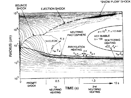
Figure 34: Time development of a type II supernova explosion after core bounce. As the nuclear matter is over-compressed in the collapse, a rebounce occurs and produces a shock wave (from [239]).

7.1.1 General remarks

The emitted neutrino spectrum consists basically of two parts. The first one is a peak of $\nu_{e}$ resulting from the deleptonisation period (eq. 112) and lasting only a few ms. During the collapse phase the core becomes opaque even for neutrinos and they diffuse within the core. The outgoing shock wave dissociates the infalling iron nuclei, increasing the mean free path for the neutrinos which pile up behind the shock. When the shock traverses the neutrinosphere (defined in a similar sense like the photosphere of the sun) all this $\nu_{e}$ will be emitted at once. The mean energy is relatively high $\langle E_{\nu}\rangle\approx 15$MeV, but the total energy released is only about $10^{51}$ erg. The second contribution comes from the Kelvin-Helmholtz cooling phase of the proto-neutron star acting as blackbody source and producing neutrinos dominantly by bremsstrahlung. All flavours are emitted in more or less equal numbers (Fig.35) within a few seconds. Because $\nu_{\mu}$ and $\nu_{\tau}$ have no charged current interactions they have a lower opacity and decouple at higher temperature and density. Also the opacity for $\bar{\nu}_{e}$ is lower than for $\nu_{e}$ because less protons are available and the opacity is dominated by $\mbox{$\nu_{e}$}+n\rightarrow p+e^{-}$ and $\mbox{$\bar{\nu}_{e}$}+p\rightarrow n+e^{+}$ respectively. Therefore one typically finds $\langle\mbox{$E_{\nu}$}\rangle$ = 10 - 12 MeV ($\nu_{e}$ ), $\langle\mbox{$E_{\nu}$}\rangle$ = 14 - 17 MeV ($\bar{\nu}_{e}$ ) and $\langle\mbox{$E_{\nu}$}\rangle$ = 24 - 27 MeV ($\nu_{\mu}$ ,$\nu_{\tau}$ ). Because the energy is approximately equipartitioned between the flavours, the fluxes behave as $\Phi(\mbox{$\nu_{e}$})>\Phi(\mbox{$\bar{\nu}_{e}$})>\Phi(\mbox{$\nu_{\mu}$},\mbox{$\nu_{\tau}$})$.

Figure 35: Time evolution of the neutrino luminosity and average energy of a supernova explosion model from [240]. The core bounce is 3-4 ms before the neutronisation burst of $\nu_{e}$ (from [240]).

The neutrino spectrum might well be described by a Fermi-Dirac shape

$$\frac{dL_{\nu}}{d\mbox{$E_{\nu}$}}\propto\frac{\mbox{$E_{\nu}$}^{3}}{1+exp(\mbox{$E_{\nu}$}/T_{\nu}-\eta_{\nu})}$$ (113)

where $\eta_{\nu}$ is a degeneracy parameter. A detailed study of the time evolution of the neutrino luminosity is rather complex and depends on many parameters like the equation of state , the mass of the collapsed core at bounce, the amount of postbounce accretion and the temperature profile after collapse. So far the only event which could be detected is SN 1987A .
In addition past supernovae could create a relic neutrino background which is discussed in [241, 242]. The total integrated flux predicted by Malaney[241] using the redshift evolution of HI-gas and the associated star formation rate is between 2-5.4 $cm^{-2}s^{-1}$ which is a factor of 10 less than previous estimates of [243, 244]. The predicted spectrum has a peak in the region 2-5 MeV which is significantly due to supernovae with redshifts larger than 1. Unfortunately the background of terrestrial reactors, solar and atmospheric neutrinos will make a detection in this region very unlikely. Experiments like Super-Kamiokande therefore have to search in the region 15-40 MeV, where the theoretical predictions for the supernova background fluxes are approximately the same.

7.1.2 SN 1987A

On February 23, 1987 the blue supergiant Sanduleak -69 202 exploded in the Large Magellanic Cloud at a distance of about 50 kpc [245]. For the first time neutrinos could be detected, bringing theoretical supernova model calculations in the regime of experimental verification. Four detectors claim observation of the neutrino burst, namely IMB [246, 247], Kamiokande [248, 249], the Baksan Scintillator Telescope [250] and the Mont Blanc Liquid Scintillator detector [251]. The Mont Blanc detection happened about 5 h earlier than the detection of the other experiments. Because of the relative low energy of the events, the non-observation of any signal during this period in the much larger water-Cerenkov detectors and a missing astrophysical scenario for producing two neutrino bursts, this detection is normally considered as a background fluctuation.
The relevant interaction processes in the water detectors are $\mbox{$\bar{\nu}_{e}$}p\rightarrow ne^{+}$, $\nu e-\nu e$ elastic scattering and $\mbox{$\nu_{e}$}\mbox{${}^{16}O$ }\rightarrow\mbox{${}^{16}N$ }+e^{-}$ which becomes the dominant contribution for $\nu_{e}$ for $E_{\nu}$ larger than about 30 MeV (Fig.36).

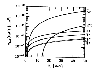
Figure 36: Different cross sections involved in the detection of supernova neutrinos. By far the largest cross section is $\mbox{$\bar{\nu}_{e}$}p\rightarrow ne^{+}$ (from [252]).

For the scintillator detectors the ${}^{16}O$ reaction is absent but at $E_{\nu}$ larger than about 30 MeV the reaction $\mbox{$\nu_{e}$}\mbox{${}^{12}C$ }\rightarrow\mbox{${}^{12}N$ }+e^{-}$ contributes. By far the largest cross section is $\mbox{$\bar{\nu}_{e}$}p\rightarrow ne^{+}$ resulting in an isotropic event distribution and is suggesting that all observed events are due to $\bar{\nu}_{e}$ interactions.
The observed numbers of neutrinos are 11 events within 12 s (Kamiokande), 8 events in 5.5 s (IMB) and 5 events in 14 s (Baksan). Some events were already attributed to background and are not included. A recent detailed maximum likelihood analysis was done by Loredo and Lamb as described in [252]. Their best-fit values are 16.9 events plus 5.6 background for Kamiokande, 4 events at IMB and 1.8 plus 1 background at Baksan. A two component cooling scheme consisting of the Kelvin Helmholtz cooling plus a low energy component which mimics the neutrinos emitted during the stalled shock-phase results in a neutrinosphere of 18 km and a total binding energy of $3.08\cdot 10^{53}$ erg in good agreement with theoretical expectations.
The observed signals contain some ”anomalies”. First of all there is a discrepancy in the neutrino energies between Kamiokande and IMB which imply a harder spectrum for IMB. Because of the rather high threshold, IMB is sensitive to the high-energy tail of the assumed neutrino spectrum, which might have substantial uncertainties. A second point is the large 7s gap between the first 8 and last 3 events of Kamiokande. This might be a statistical fluctuation because IMB and Baksan do have events in this period. The most striking is the deviation from isotropy which is expected if all events are due to $\bar{\nu}_{e}$ interactions (Fig.37). The observed distribution is only at the per cent level in agreement with isotropy and an explanation for this fact is still missing.

Figure 37: Energy and observed angle as a function of time for IMB (white), Kamiokande (black) and Baksan (stars).

Concerning neutrino properties several things could be learned even by the low statistics of the observed event numbers. Because of the observed pulse length, mass effects on the propagation from SN 1987A to the earth restrict the neutrino mass to a conservative upper limit of about 25 eV, which could be improved under certain model dependent assumptions down to 13 eV. Because the measured number of events corresponds to the theoretical expectation, rather stringent bounds on neutrino decay can be given, implying

$$\frac{\mbox{$E_{\nu}$}}{m_{\nu}}\tau_{\nu_{e}}\geq 5\cdot 10^{12}s.$$ (114)

The radiative decay channel is additionally limited by the Solar Maximum Mission which did not observe any signal which could be related to the neutrino burst of SN 1987A [253]. This was confirmed by a systematic search for the radiative decay of neutrinos coming from Type II supernova using COMPTEL data [254]. A stringent bound also exists on the electric charge of the neutrinos. An electric charge would cause longer travel distances for lower energy neutrinos because effects due to the galactic magnetic field are more important to them. Therefore the charge of the neutrinos can be bounded by $Q_{\nu}<10^{-17}e$.
Neutrino oscillations and the MSW-effect might also play a significant role in supernovae. Oscillations in the channel $\nu_{e}$ - $\nu_{X}$ are able to reduce the prompt signal significantly. A detailed analysis, assuming $\Delta m^{2}$ $\stackrel{{\scriptstyle<}}{{\sim}}3\cdot 10^{-4}eV^{2}(\mbox{$E_{\nu}$}/10MeV)$ to allow for a resonance outside the neutrinosphere , reveals that a probability for a conversion of more than 50 % already occurs for $\mbox{$\Delta m^{2}$}sin^{3}2\theta\stackrel{{\scriptstyle>}}{{\sim}}4\cdot 10^{-9}eV^{2}(\mbox{$E_{\nu}$}/10MeV)$ extending to large $\Delta m^{2}$ values. Furthermore if the resonance lies outside the neutrinosphere and within the shock wave (which is valid for neutrino masses in the region of order 10 eV or above and therefore a cosmological interesting region) the higher energy $\nu_{\mu}$ and $\nu_{\tau}$ , if converted to $\nu_{e}$ could help to revive the stalled shock [255]. The minimum mixing angle necessary is $sin^{2}2\theta$ $\stackrel{{\scriptstyle>}}{{\sim}}$ $10^{-8}$ $E_{\nu}$ /10 MeV. This would imply a reduction of the prompt $\nu_{e}$ pulse. The oscillation of $\nu_{e}$ could furthermore influence the creation of r-process events. The hot bubble between the settled neutron star and the escaping shock wave a few seconds after the core bounce seems to be a reliable place for r-process nucleosynthesis. The p/n-ratio in the bubble is governed by the reactions $\mbox{$\nu_{e}$}n\leftrightarrow pe^{-}$ and $\mbox{$\bar{\nu}_{e}$}p\leftrightarrow ne^{+}$. Because neutrinos are much more common than electrons and positrons, the p/n ratio is ruled by the spectra and fluxes of the neutrinos . This normally results in a neutron rich environment, because $\bar{\nu}_{e}$ are more energetic than $\nu_{e}$ . Oscillations of $\nu_{\mu}$ and $\nu_{\tau}$ to $\nu_{e}$ outside the neutrinosphere could make the $\nu_{e}$ flux more energetic than the $\bar{\nu}_{e}$ . Even a 10 % oscillation effect would drive the medium to a proton-rich state. The parameters obtained to allow the r-process also lie in the cosmological region requiring $\Delta m^{2}$ $\stackrel{{\scriptstyle>}}{{\sim}}$ 2 eV and $sin^{2}2\theta$ $\stackrel{{\scriptstyle<}}{{\sim}}$ $10^{-5}$ for $\nu_{e}$ - $\nu_{\mu}$ ,$\nu_{\tau}$ oscillations [256]. At smaller $\Delta m^{2}$ the oscillation effect has no impact on the r-process because it occurs at too large radii.

7.1.3 Experimental status

The experimental observation of SN 1987A launched several new searches for supernova neutrinos. Besides specially developed detectors, basically all new real-time solar neutrino detectors like Super-Kamiokande , ICARUS and SNO will be able to see such neutrinos. The predicted count rate for Super-Kamiokande of a galactic supernova at a distance of 10 kpc is 5000 - 10000 $\bar{\nu}_{e}$ interactions! Such an event would open the possibility to explore the mass of $\nu_{\mu}$ and $\nu_{\tau}$ down to 50 eV by using the neutral current excitation of ${}^{16}O$ [257]. SNO might be especially valuable because of the NC desintegration of D (eq. 104) which will be dominated by $\bar{\nu}_{\mu}$ and $\bar{\nu}_{\tau}$ . Detectors like LVD and MACRO also offer additional discovery potential. The main component of all detectors will still be the $\bar{\nu}_{e}$ detection. A completely different scheme which is mainly sensitive to $\nu_{\mu}$ and $\nu_{\tau}$ is the SNBO idea [258] recently put into a realistic detector design in form of OMNIS [259]. The basic idea of [258] is NC excitation of nuclei

$$\nu A(Z,N)\rightarrow A^{\ast}(Z,N)\rightarrow A(Z,N-1)+\nu+n$$ (115)

via the de-excitation by neutron emission. As target material large underground areas of rock or salt should be equipped with neutron detectors. The efficiency can be increased by using caverns in the rock for neutron detection. With about 200 tons of a Gd loaded scintillator, event rates of more than 2000 neutrino interactions for a galactic supernova in a distance of 8 kpc seem feasible. Because of their higher energy, the signal would be dominated by $\nu_{\mu}$ and $\nu_{\tau}$ interactions. An extension to extragalactic supernovae (an increase to about 4 Mpc in sensitivity would imply about 1 supernova per year) unfortunately seems unrealistic at present times.

7.2 Neutrinos from other astrophysical sources

After describing experimentally observed astrophysical neutrino sources like the sun and supernovae there might be other sources of neutrinos of even higher energies ($E_{\nu}>100MeV$). Their existence may be closely related to the recently discovered TeV- $\gamma$-sources and the sources of cosmic rays. Neutrinos are produced via pp-collisions or photoproduction in cosmic beam-dump experiments due to the decay of the created charged pions and kaons. The associated production of neutral pions allows a relation between expected photon and neutrino fluxes (eq.118). The threshold for pion-photoproduction is rather high and the minimal proton energy required is given by

$$E_{p}=\frac{(2m_{p}+m_{\pi})\cdot m_{\pi}}{4E_{\gamma}}=7\cdot 10^{16}(E_{\gamma}(eV))^{-1}(eV)$$ (116)

Using the cosmic microwave background (CMB) as target photons, a threshold energy for the proton of $E_{p}\approx 5\cdot 10^{19}$ eV results (GZK-cutoff) [260, 261]. In contrast to photons and protons, neutrino propagation is not influenced by attenuation or deflection by magnetic fields. Neutrinos give direct information on the source location and might reveal sources which have no $\gamma$-counterpart. Even more, while high energy photons are influenced by $\gamma\gamma\rightarrow e^{+}e^{-}$ reactions on the CMB and in the TeV-region by the same reaction with the presently unknown IR-background, they have a limited range for detection, whereas neutrinos can be observed to largest distances.
The main detection reaction on earth will be upward going muons discussed in more detail in chapter 7.2.2.

7.2.1 Sources and predictions

Several galactic and extragalactic sources are discussed for highest energy neutrinos most of them are also investigated for creating and accelerating cosmic rays . For a detailed discussion of sources see [262]. The spectral shape of the primary cosmic rays follows a power law according to

$$\Phi(E)\propto E^{-(\gamma+1)}$$ (117)

where the spectrum observed on earth is characterised by $\gamma\approx 1.7$ (for E $<10^{15}$ eV) then steepening to $\gamma\approx 2$ (”knee region”) and then changing again at $10^{19}$ eV (”ankle”). This spectrum is steeper than the accelerated one because of the energy dependence of cosmic ray diffusion in the galaxy. Neutrinos produced in interactions with the interstellar gas should follow the shape of the primary cosmic ray spectrum up to highest energies. On the other hand, if the production occurs at the acceleration site, there is no diffusion effect and the spectral shape follows the hard source spectrum ($\gamma\approx 2-2.2$). From the above mentioned interaction mechanisms it is clear that there are point sources in the sky and a diffuse component. Two examples of possible galactic point sources are X-ray binaries (a compact object like a neutron star or black hole is accreting matter from a non-compact companion) like Cygnus X-3 or young supernova remnants. To produce a detectable signal of a few upward going muons per year in a $10^{5}m^{2}$ detector, X-ray binaries have to convert almost all energy in the acceleration of protons. The supernova remnants on the other hand are rare events and typically produce a signal only during a period on the scale of years after the explosion. A guaranteed source for neutrino production is the galactic disc, where a diffuse photon background due to interactions of cosmic ray protons with interstellar matter could be observed by EGRET on CGRO [263]. If neutrinos are coming from $\pi$-decay like the observed photons the neutrino flux can be determined by [262]

$$\Phi_{\nu}=C\cdot\left(1-(\frac{m_{\mu}}{m_{\tau}})\right)^{\alpha-1}\frac{1}{1-A_{\gamma}}$$ (118)

where $A_{\gamma}$ is the energy dependent photon attenuation dominated by $\gamma\gamma\rightarrow e^{+}e^{-}$. A second source is our sun, because of cosmic ray interactions within the solar atmosphere. Moreover the sun could trap neutralinos $\chi$ as dark matter in its interior. Their $\chi{\bar{\chi}}$-annihilation can be a source of high energy neutrinos. Predictions for the neutrino -flux on earth for a 500 GeV neutralino $\chi$ are of the order $\Phi_{\nu}\approx 2\cdot 10^{-8}\mbox{$cm^{-2}s^{-1}$ }$.
The most prominent extragalactic source candidates are active galactic nuclei (AGN) and gamma ray bursters (GRBs). The present -here simplified- picture of AGN consists of a central supermassive black hole ($\approx 10^{8}-10^{10}M_{\odot}$) accreting matter near its Eddington limit. The accelerated matter will form a hot, dense plasma and will be partly sucked into the black hole and partly redirected by magnetic fields forming two opposite directed jets perpendicular to the accretion disc. In this scenario there are basically two ways to accelerate particles by shock acceleration and to produce a neutrino flux. The first possibility is near the central engine as described in [262]. Energy losses take place due to processes like $p\gamma\rightarrow\Delta^{+}\rightarrow n\pi^{+}$ and $p\gamma\rightarrow p+e^{+}+e^{-}$ in the radiation field as well as pp-collisions in the gas. Both processes give rise to photons and neutrinos , but the produced photons from $\pi^{0}$-decay cascade down and are released as X-rays, because the central region is optically thick for energies larger than $\sim$ 5 MeV. Crucial for this mechanism to work are the assumptions on proton propagation and confinement in the core region. Note however, that the majority of X-ray emitting AGN does not show a nonthermal X-ray spectrum (cascade origin) but a thermal spectrum peaking at $\sim$ 100 keV. The second source which might explain the observation of TeV-photons from several extragalactic sources like Markarian 421 are the highly relativistic jets. It is of outstanding interest to know whether the observed photons are created from inverse Compton scattering or synchrotron emission of accelerated electrons or from photoproduction of pions from accelerated protons [264]. The observation of neutrinos would help to clarify the situation.
By integrating over all cosmological AGN, one should also see a diffuse background of neutrinos in the same way as the diffuse $\gamma$-ray background is obtained. According to Stecker [265] it remains flat up to about $10^{7}$ GeV and then starts to fall steeply. For energies larger than about $3\cdot 10^{4}$ GeV it becomes dominant with respect to atmospheric neutrinos. While different models agree more or less in their prediction at the high energy end of $\approx 10^{10}$ GeV, orders of magnitude differences exist in the lower energy region around $10^{5}$ GeV. Predicted fluxes of several models can be found in [266, 267, 268, 269, 270].

Figure 38: Predicted diffuse isotropic neutrino flux from the sum over all active galactic nuclei predicted by various models. Also shown is the horizontal and vertical atmospheric neutrino flux, dominating in the region below 1 TeV. Two different models for prompt neutrinos from charm decay of TIG [160] and model D of Zas et al. [271] are also shown (from [270]).

A combined high energy neutrino spectrum for point and diffuse sources can be seen in Fig. 38. The typical estimates for their detection via upward going muons are in the order of 0.1-10 events per year for a 0.1 km² detector with rather large uncertainties. A flux limit of $d\Phi/dE_{\nu}<7\cdot 10^{-13}GeV^{-1}\mbox{$cm^{-2}s^{-1}$ }sr^{-1}(90\%CL)$ for $\nu_{\mu}$ in the energy region of $E_{\nu}\approx$ 2.6 TeV exist from the Frejus-experiment [272], already ruling out the model of Szabo et al. [267] and the maximal flux predictions of Bhattacharjee et al. [273].
Other partially more exotic sources of high energy neutrinos might exist. Neutrinos associated with GRBs are discussed in Waxmann et al. [274]. Further scenarios are annihilation or decay of superheavy particles like the neutralino $\chi$ [275]. Also evaporating black holes and radiation from topological defects like cosmic strings might be sources for neutrinos [273, 276].

7.2.2 Experimental search

From the flux estimates of the last chapter, it is rather clear that very large detectors are required. The proposed detection reaction for the VHE-neutrinos are $\nu_{\mu}$ CC reactions producing upward going muons . The corresponding cross-sections are shown in Fig. 39. The $\nu_{\mu}$ CC cross section is given by

$$\frac{d^{2}\sigma}{dxdy}=\frac{2G_{F}^{2}m\mbox{$E_{\nu}$}}{\pi}(\frac{m_{W}^{2}}{Q^{2}+m_{W}^{2}})(xq(x,Q^{2})+x\bar{q}(x,Q^{2})(1-y)^{2})$$ (119)

with $q(x,Q^{2}),\bar{q}(x,Q^{2})$ as the quark distribution functions, the Bjorken variable $x=Q^{2}/2m\nu$, $m$ the nucleon mass and $y=(\mbox{$E_{\nu}$}-E_{\mu})/\mbox{$E_{\nu}$}$. Towards higher energies the contribution from the presently unknown small x-region is becoming more important and theoretical extrapolations have to be used [277].

Figure 39: Total as well as NC and CC cross sections for high enery neutrinos (left) and antineutrinos (right) (from [277]).

To face the background from the atmospheric neutrino flux, which is at lower energies typically a factor of $10^{6}$ larger than cosmic sources (but falls off steeper towards higher energies), only muons transversing the detector from below can be used (upward going muons). Therefore cosmic sources of interest have to stay below the horizon for a significant time.
The effective detector size for detecting upward going muons can be enlarged because the surrounding material can be used as an additional target. The energy loss rate of muons due to ionisation and catastrophic losses like bremsstrahlung, pair-production and hadroproduction is given by

$$\frac{dE_{\mu}}{dX}=-\alpha-\frac{E_{\mu}}{\xi}$$ (120)

with the critical energy $\epsilon=\alpha\xi\approx 500$ GeV. This results in a range R of ($\xi\approx$ 2 km.w.e.)

$$R\approx\xi ln(1+\frac{E_{0}}{\epsilon})$$ (121)

For high energy muons the radiation losses are dominant, resulting in a change of energy dependence of the range from linear to logarithmic. For a muon with initial energy larger than 0.5 TeV the range exceeds 1 km. For neutrino energies larger than about 40 TeV the interaction length becomes smaller than the diameter of the earth resulting in a shadowing effect.
The existing underground detectors like MACRO, Super-Kamiokande and LVD have too small sizes to measure statistically significant signals. Therefore natural resources of water and ice are used to detect the Cerenkov-light of the passing muon. After the termination of DUMAND, the Lake Baikal experiment (water) and AMANDA (ice) are the most advanced projects.
The Baikal neutrino telescope (NT) is located in a depth of 1.1 km at a distance of 3.6 km from the shore [278]. The final setup of NT-200 is finished recently and consists of 8 strings forming a heptagonal array of seven strings around a central string. It consists of 192 pairs of 8” photomultipliers arranged in a distance of 5 and 7.5 m along the strings. This rather small spacing allows a relatively low energy threshold of about 10 GeV. Besides the low threshold the main advantages of the experiment are the relatively cheap deployment of tubes, because the frozen lake offers a good platform for deployment and Lake Baikal is a sweet-water sea containing no ${}^{40}K$ whose decay would produce background. The effective area is between $1000-5000m^{2}$ depending on energy and an increase of the effective area by a factor 20-50 is under consideration. Clear upward going muons have been observed.
AMANDA [279, 280] is at present operating 300 8” photomultipliers in the antarctic ice in a depth of 1500 - 2000 m. The basically bubble-free ice offers extraordinary optical properties, e.g. the absorption length for $\lambda\approx 500$ nm is around 100 m and the scattering length about 25 m. The detector offers an effective area of $10^{4}m^{2}$ with a mean angular resolution of 2.5^o. An upgrade to a 1 km³ detector (ICECUBE) which would consist of about 5000 photomultipliers mounted on 80 strings with a spacing of about 100 m is under consideration. Good candidates for upward going muons have been observed by AMANDA.
Two further water experiments in the Mediterranean are in a kind of preparation phase, namely NESTOR [281] near Greece, in a depth of 3800 m and ANTARES [282] near Toulon (France), in a depth of 2000m.
Associated with two of the projects mentioned above are alternative experiments using different detection techniques. They are called RICE [283] (together with AMANDA) and SADCO [284] (together with NESTOR). They rely on detection of radio and acoustic signals produced if $E_{\nu}\stackrel{{\scriptstyle>}}{{\sim}}$ 1 PeV. In the acoustic case, the produced shower particles in the $\nu_{e}$ - interaction lose energy through ionisation leading to a local heating and density change. The density change propagates as sound waves through the medium and can be detected with an array of detectors like hydrophones allowing also a reconstruction of the event by measuring the arrival times and amplitudes. The second method uses the effect of coherent radio Cerenkov radiation which is produced as long as the wavelength is large with respect to the spatial extension of the shower [285]. The neutral pions create an electromagnetic shower of size 1m in ice via their $\pi^{0}\rightarrow\gamma\gamma$ decay, therefore producing frequencies in the region 100 Mhz - 1 GHz.
For detection of very high energetic neutrinos the reaction

$$\bar{\mbox{$\nu_{e}$}}+e^{-}\rightarrow W^{-}\rightarrow hadrons$$ (122)

can be used which shows a resonance behaviour (Glashow - resonance) at $s=m_{W}^{2}$, meaning $E_{\nu}=6.3\cdot 10^{6}$ GeV. The $\bar{\nu}_{e}e$ cross section at the resonance is about a factor 30 larger than the corresponding $\nu$N cross section (Fig. 40).

Figure 40: Glashow resonance in the $\bar{\mbox{$\nu_{e}$}}e$ cross section. The curves correspond, in the low energy region from highest to lowest, to $(i)\bar{\mbox{$\nu_{e}$}}e\rightarrow$ hadrons $(ii)\mbox{$\nu_{\mu}$}e\rightarrow\mu\mbox{$\nu_{e}$}{}(iii)\mbox{$\nu_{e}$}e\rightarrow\mbox{$\nu_{e}$}e{}(iv)\mbox{$\bar{\nu}_{e}$}e\rightarrow\mbox{$\bar{\nu}_{\mu}$}\mu{}(v)\mbox{$\bar{\nu}_{e}$}e\rightarrow\mbox{$\bar{\nu}_{e}$}e{}(vi)\mbox{$\nu_{\mu}$}e\rightarrow\mbox{$\nu_{\mu}$}e{}(vii)\mbox{$\bar{\nu}_{\mu}$}e\rightarrow\mbox{$\bar{\nu}_{\mu}$}e$ (from [277]).

The field of high energy neutrino astrophysics is still in its initial phase but will provide important information in the future.

7.3 Relic neutrinos

The thermal history of the universe according to the big bang model predicts not only a photon background but also a neutrino background. While the photons are observed as the cosmic microwave background, the neutrino background is still undetected. The temperatures of both are related by the relation

$$\mbox{$T_{\nu}$}=(\frac{4}{11})^{\frac{1}{3}}\mbox{$T_{\gamma}$}$$ (123)

where $T_{\gamma}$ is measured quite accurately by COBE to be $T_{\gamma}$ = 2.728 $\pm$ 0.004 [286], thus predicting a neutrino background temperature of 1.95 K. The total number density and matter density (the flavour densities are one third) are then given by

$$n_{\nu}=\frac{3g_{\nu}}{22}n_{\gamma}=337cm^{-3}$$ (124)

$$\rho_{\nu}=\frac{7g_{\nu}}{8g_{\gamma}}(\frac{4}{11})^{\frac{4}{3}}\rho_{\gamma}=0.178\frac{eV}{cm^{3}}$$ (125)

with the statistical weights $g_{\gamma}=2,g_{\nu}$ = 2 for Majorana neutrinos and light ($m_{\nu}$ $\stackrel{{\scriptstyle<}}{{\sim}}$ 300 keV) Dirac neutrinos , otherwise $g_{\nu}$ = 4. The mean energy of the neutrinos today is $5.28\cdot 10^{-4}$ eV making a detection extremely difficult. The neutrino contribution to the matter density is given as

$$\Omega_{\nu}=\frac{\rho_{\nu}}{\rho_{c}}=5.32\cdot 10^{-3}\frac{g_{\nu}}{h^{2}}\frac{m_{\nu}}{eV}$$ (126)

where $\rho_{c}$ is the critical density and $h=H_{0}/100kms^{-1}Mpc^{-1}$ the normalised Hubble-constant. For $m_{\nu}$ $\stackrel{{\scriptstyle>}}{{\sim}}$ 1 MeV neutrinos become non-relativistic and their density is suppressed by a Boltzmann-factor. The behaviour of $\Omega_{\nu}$ as a function of $m_{\nu}$ is shown in Fig.41.

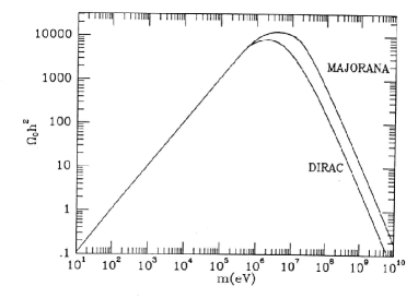
Figure 41: Neutrino contribution to $\Omega$ as a function of the neutrino mass. Two regions remain for stable neutrinos to be cosmological of interest. Either below 100 eV (acting as hot dark matter) or above 5 GeV (acting as cold dark matter). Otherwise they have to be unstable because they would overclose the universe.

As can be seen, stable neutrinos only exist for $m_{\nu}$ $\stackrel{{\scriptstyle<}}{{\sim}}$ 100 eV and for $m_{\nu}$ $\stackrel{{\scriptstyle>}}{{\sim}}$ 2(5) GeV in the Dirac (Majorana ) case (Lee-Weinberg-bound). Both allowed mass regions offer massive neutrinos as good dark matter candidates, either as hot dark matter (neutrinos in the eV-range) or as cold dark matter (neutrinos in the GeV range) [287]. Pure cold dark matter models predict to many galaxy clusters, which can be avoided by including a hot component. Because of their free streaming in the early universe, light neutrinos wash out perturbations on small scales, reducing the power there. A mixed hot and cold dark matter model with $\Omega=1$ and 5 eV neutrinos contributing $\Omega_{\nu}\approx 0.2$ for $h=0.5$ seems to be a good description of the COBE normalised power spectrum and the observed large scale structure. This can be improved if the hot component consists of two neutrino flavours having a mass of about 2.5 eV [288]. GeV neutrinos as cold dark matter are bounded by double beta decay experiments excluding Dirac - neutrinos with standard interactions between 26 GeV and 4.7 TeV as the dominant component [289, 290]. The linear contribution for light neutrinos to $\Omega_{\nu}$ (eq.126) can be converted in a neutrino mass bound. The condition not to overclose the universe requires for stable neutrinos

$$\sum_{i}m_{i}(\frac{g_{\nu}}{2})=94eV\Omega_{\nu}h^{2}$$ (127)

which is orders of magnitude more stringent for $\nu_{\mu}$ and $\nu_{\tau}$ than laboratory limits. The same condition also allows only certain ranges of lifetimes for unstable neutrinos [12]. Radiative decay channels are additionally restricted because the created photons would otherwise influence the thermodynamic evolution too strongly. Other decay channels might be possible. The most common ones discussed for heavy neutrino decays are

$$\nu_{H}\rightarrow\nu_{L}+\gamma$$ (128)

$$\nu_{H}\rightarrow\nu_{L}+l^{+}l^{-}\quad l=e,\mu$$ (129)

$$\nu_{H}\rightarrow\nu_{L}+\bar{\nu}_{L}+\nu_{L}$$ (130)

$$\nu_{H}\rightarrow\nu_{L}+\chi$$ (131)

where $\chi$ corresponds to a light scalar like the majoron. Bounds on the radiative decay mode exist from reactor experiments [291], LAMPF [292] and from SN 1987A [293]. The decay mode involving $e^{+}e^{-}$-pairs is restricted in the region 1-8 MeV by reactor data [294] and at higher energies by accelerator searches (see [295]).
Experimental detection of the neutrino background will be extremly difficult. One of the suggestions is to take advantage of coherence in $\nu N$-scattering and by using cryogenic detectors, but also this proposal is far from practical realisation. A chance might be that eq.125 is modified during decoupling in the early universe by incomplete annihilation and finite temperature QED-effects, which might increase $\rho_{\nu}$ by about 1 % [296]. This effect might be detectable in the future satellite missions MAP and PLANCK by its influence on the anisotropies in the cosmic microwave background [297].

8 Conclusions and outlook

The question whether neutrinos have a non-vanishing rest mass influences research areas from particle physics up to cosmology, but is still an open question. At present all hints for neutrino masses are connected with neutrino oscillation effects namely the solar neutrino deficit, the atmospheric neutrino anomaly and the evidence from LSND . The involved $\Delta m^{2}$ scales are in the $10^{-5}(10^{-11})eV^{2}$ MSW-(vacuum)solution, $10^{-3}eV^{2}$ and eV-region respectively. Several theoretical models have been developed to describe these evidences in a consistent way [298, 299]. With the appearance of the new CHOOZ and Super-Kamiokande results most of these models seem to be ruled out. Moreover to explain all data in addition to the three standard neutrinos a new sterile neutrino seems necessary [300, 301, 302, 303]. The scheme of Barger et al. [302] proposes a nearly degenerate $\nu_{\mu}$ and $\nu_{\tau}$ in the eV-range and much lighter $\nu_{e}$ and $\nu_{S}$. The splitting between the eV-states and the light ones is determined by LSND data. The atmospheric anomaly can be solved by $\nu_{\mu}$ - $\nu_{\tau}$ oscillations and both can act as hot dark matter. The solar neutrino problem is solved by $\nu_{e}$ - $\nu_{S}$ oscillations which require the $\nu_{S}$ to be slightly heavier than $\nu_{e}$ .
The right answer will hopefully be given in the future, because of an increasing number of new experiments.

References

- [1] W. Pauli, Fünf Arbeiten zum Ausschlieungsprinzip und zum Neutrino, Texte zur Forschung Vol. 27, Wissenschaftliche Buchgesellschaft Darmstadt 1977, W. Pauli, On the earlier and more recent history of the neutrino (1957) in: Neutrino physics, ed. K. Winter, Cambridge University Press, 1991
- [2] F. Reines, C.L. Cowan, Nature 178, 446 (1956)
- [3] G. Danby et al., Phys. Rev. Lett. 9, 36 (1962)
- [4] D. Abbaneo et al., CERN-PPE/97-154
- [5] H. Weyl, Z. Phys. 56, 330 (1929)
- [6] E. Majorana, Nuovo Cimento 14, 171 (1937)
- [7] S.M.Bilenky, S.T. Petcov, Rev. Mod. Phys. 59, 671 (1987), Rev. Mod. Phys. 60, 575 (1988) (err), Rev. Mod. Phys. 61, 169 (1989) (err)
- [8] M. Gell-Mann, P. Ramond, R. Slansky, in Proc. Supergravity, ed. P. van Nieuwenhuizen, D. Freedman, North Holland, 1979, p.315
- [9] T. Yanagida, Prog. Theo. Phys. 64, 1103 (1980)
- [10] P. Langacker in Neutrinos ed. H.V. Klapdor, Springer 1988
- [11] S. Bludman et al., Phys. Rev. D 45, 1810 (1992)
- [12] R.N. Mohapatra, P. Pal, Massive neutrinos in physics and astrophysics, World Scientific, 1991
- [13] A. Zee, Phys. Lett. B 93, 389 (1980), Phys. Lett. B 161, 141 (1985)
- [14] L. Wolfenstein, Nucl. Phys. B 175, 93 (1980)
- [15] K.S. Babu, Phys. Lett. B 203, 132 (1988)
- [16] J.C. Pati, A. Salam, Phys. Rev. D 10, 275 (1974)
- [17] R.N. Mohapatra, Proc. ECT Workshop on double beta decay and related topics, Trento, eds. H.V. Klapdor-Kleingrothaus and S.Stoica, World Scientific, 1995 p.44
- [18] R.N. Mohapatra, G. Senjanovic, Phys. Rev. D 23, 165 (1981)
- [19] A. Franklin, Rev. Mod. Phys. 67, 457 (1995)
- [20] F.E. Wietfeldt, E.B. Norman, Phys. Rep. 273, 149 (1996)
- [21] E. Holzschuh, Rep. Prog. Phys. 55, 851 (1992)
- [22] E.W. Otten, Nucl. Phys. B (Proc. Suppl.) 38, 26 (1995)
- [23] V.M. Lobashev et al., Nucl. Instrum. Methods A 240, 305 (1985)
- [24] A. Picard et al., Nucl. Instrum. Methods B 63, 345 (1992)
- [25] A.M. Swift et al., Proc. Neutrino’96, World Scientific, 1997, p.278
- [26] P. Meunier in astro-ph/9801320
- [27] A. deRujula, Nucl. Phys. B 188, 414 (1981)
- [28] P.T. Springer, C.L.Bennett, R.A. Baisden, Phys. Rev. A 35, 679 (1987)
- [29] K. Assamagan et al., Phys. Rev. D 53, 6065 (1996)
- [30] B. Jeckelmann et al., Phys. Lett. B 335, 326 (1995)
- [31] S. Lenz et al., Phys. Lett. B 416, 50 (1998)
- [32] H. Albrecht et al., Phys. Lett. B 292, 221 (1992)
- [33] R. Ammar et al., Phys. Lett. B 431, 209 (1998)
- [34] G. Alexander et al., Z. Phys. C 72, 231 (1996) hep-ex/9806035
- [35] L. Passalacqua, Nucl. Phys. B (Proc. Suppl.) 55C, 435 (1997)
- [36] R. Barate et al., Europ. Phys. J. C 2, 395 (1998)
- [37] G. Gyuk, M.S. Turner, Nucl. Phys. B (Proc. Suppl.) 38, 13 (1995)
- [38] B.D. Fields, K. Kainulainen, K.A. Olive, Astroparticle Physics 6, 169 (1997)
- [39] M. Doi, T. Kotani, E. Takasugi, Prog. Theo. Phys. 69, 602 (1983)
- [40] M. Doi, T. Kotani, E. Takasugi, Prog. Theo. Phys. Suppl. 83, 1 (1985)
- [41] K.Muto, H.V. Klapdor in Neutrinos, ed. H.V. Klapdor, Springer 1988
- [42] M. Goeppert-Mayer, Phys. Rev. 48, 512 (1935)
- [43] W.H. Furry, Phys. Rev. 56, 1184 (1939)
- [44] J. Schechter, J.W.F. Valle, Phys. Rev. D 25, 2591 (1982)
- [45] E. Takasugi, Phys. Lett. B 149, 372 (1984)
- [46] H.V. Klapdor-Kleingrothaus, A. Staudt, Non accelerator particle physics, IOP Publ., Bristol 1995
- [47] F. Boehm, P. Vogel, Physics of massive neutrinos, Cambridge Univ. Press 1992
- [48] V.I. Tretyak, Y.G. Zdesenko, At. Dat. and Nucl. Dat. Tab. 61,43 (95)
- [49] G. Heusser, Ann. Rev. Nucl. Part. Phys. 45, 543 (1995)
- [50] E. Fiorini et al. , Phys. Lett. B 45, 602 (1967)
- [51] M. Guenther et al., Phys. Rev. D 55, 54 (1997)
- [52] F.T. Avignone, Proc. Neutrino’96, World Scientific, 1997 p.361
- [53] K. You et al. , Phys. Lett. B 265, 53 (1991)
- [54] A.S. Georgadze, Phys. Atom. Nucl. 58, 1093 (1995)
- [55] E. Fiorini, Proc. Neutrino’96, World Scientific, 1997 p.352
- [56] J. Farine, Proc. Neutrino’96, World Scientific, 1997 p.347
- [57] H. Ejiri, Proc. Neutrino’96, World Scientific, 1997 p.342
- [58] R. Arnold et al., Nucl. Phys. A 636, 209 (1998)
- [59] T. Kirsten, Proc. Int. Symp. on Nuclear beta decays and neutrinos, eds. T. Kotani, H. Ejiri, E. Takasugi, Osaka 1986 , World Scientific p.81
- [60] P. Vogel, M.R. Zirnbauer, Phys. Rev. Lett. 57, 3148 (1986)
- [61] K. Grotz, H.V. Klapdor, Weak interactions in nuclear-,particle- and astrophysics, Adam Hilger, Bristol 1990
- [62] J. Suhonen, O. Civitarese, Phys. Rep. 300, 123 (1998)
- [63] A. Staudt, K. Muto, H.V. Klapdor-Kleingrothaus, Europhys. Lett. 13, 31 (1990)
- [64] T. Kirsten, W. Gentner, O.A. Schaeffer, Z. Phys. 202, 273 (1967)
- [65] T. Kirsten, W. Gentner, O.A. Schaeffer, Phys. Rev. Lett. 20, 1300 (1968)
- [66] W.J. Lin et al., Nucl. Phys. A 481, 477 and 484 (1988)
- [67] T. Bernatowicz et al., Phys. Rev. C 47, 806 (1993)
- [68] A.I. Turkevich, T.E. Economou, G.A. Cowen, Phys. Rev. Lett. 67, 3211 (1992)
- [69] S.R. Elliott, A.A.Hahn, M.Moe, Phys. Rev. Lett. 59, 1649 (1987)
- [70] T. Tomoda, Rep. Prog. Phys. 54, 53 (1991)
- [71] P. Vogel in Proc. ECT Workshop on double beta decay and related topics, Trento, eds. H.V. Klapdor-Kleingrothaus and S.Stoica, World Scientific, 1995 p.323
- [72] A. Faessler in Proc. ECT Workshop on double beta decay and related topics, Trento, eds. H.V. Klapdor-Kleingrothaus and S.Stoica, World Scientific, 1995 p.339
- [73] K. Muto, E. Bender, H.V. Klapdor, Z. Phys. A 39, 435 (1991)
- [74] L. Baudis et al., Phys. Lett. B 407, 219 (1997)
- [75] M. Hirsch et al., Phys. Lett. B 374, 7 (1996)
- [76] M. Hirsch, H.V. Klapdor-Kleingrothaus, S. Kovalenko, Phys. Lett. B 352, 1 (1995), Phys. Rev. D 53, 1329 (1996)
- [77] M. Hirsch, H.V. Klapdor-Kleingrothaus, S. Kovalenko, Phys. Lett. B 378, 17 (1996), Phys. Rev. D 54, 4207 (1996)
- [78] A.S. Barabash in Proc. ECT Workshop on double beta decay and related topics, Trento, eds. H.V. Klapdor-Kleingrothaus and S.Stoica, World Scientific, 1995 p.502
- [79] A.Halprin, S.T.Petcov, S.P.Rosen, Phys. Lett. B 125, 335 (1983)
- [80] K. Zuber, Phys. Rev. D 56, 1816 (1997)
- [81] M. Doi, T. Kotani, E. Takasugi, Phys. Rev. D 37, 2575 (1988)
- [82] Y. Chikashige, R.N. Mohapatra, R.D. Peccei, Phys. Rev. Lett. 45, 1926 (1980)
- [83] R. Santamaria, J.W.F. Valle, Phys. Rev. Lett. 60, 397 (1988)
- [84] G.B. Gelmini, M. Roncadelli, Phys. Lett. B 99, 411 (1981)
- [85] C.P. Burgess, J.M. Cline, Phys. Rev. D 49, 5925 (1994)
- [86] M. Hirsch et al., Phys. Lett. B 372, 8 (1996)
- [87] C.D. Carone, Phys. Lett. B 308, 85 (1993)
- [88] R.N. Mohapatra, E. Takasugi, Phys. Lett. B 211, 192 (1988)
- [89] K. Zuber, Talk presented at PASCOS’92, Ann. NY. Acad. Sci 688, 509 (1993)
- [90] J. Tanaka, H. Ejiri, Phys. Rev. D 48, 5412 (1993)
- [91] M. Guenther et al. , Phys. Rev. D 54, 3641 (1996)
- [92] E.B. Norman, M.A. DeFaccio, Phys. Lett. B 148, 31 (1984)
- [93] M. Hirsch et al., Z. Phys. A 347, 151 (1994)
- [94] A. Alessandrello et al., Phys. Lett. B 420, 109 (1998)
- [95] A.S. Barabash, Proc. Neutrino’96, World Scientific, 1997 p.374
- [96] R.S. Raghavan, Phys. Rev. Lett. 72, 1411 (1994)
- [97] E. Fiorini, private communication
- [98] H.V. Klapdor-Kleingrothaus, J. Hellmig, M. Hirsch, Journal of Physics G 24, 483 (1998)
- [99] M. Moe, Phys. Rev. C 44, R931 (1991)
- [100] L. Mitchell, Talk presented at Topical Workshop on Neutrino Physics, Adelaide 1996
- [101] B.W. Lee, R.E. Shrock, Phys. Rev. D 16, 1444 (1977)
- [102] W.J. Marciano, A.I. Sanda, Phys. Lett. B 67, 303 (1977)
- [103] P.B. Pal, Int. Journal of Modern Physics A7, 5387 (1992)
- [104] D. Krakauer et al., Phys. Lett. B 252, 171 (1990)
- [105] K. Abe et al., Phys. Rev. Lett. 58, 636 (1987)
- [106] C.S. Kim, W.J. Marciano, Phys. Rev. D 37, 1368 (1988)
- [107] M.B. Voloshin, M.I. Vysotsky, L.B. Okun, Sov. Journal of Nucl. Phys. 44, 440 (1986)
- [108] R. Barbieri, R.N. Mohapatra, Phys. Rev. Lett. 61, 27 (1988)
- [109] J.M. Lattimore, J. Cooperstein, Phys. Rev. Lett. 61, 23 (1988)
- [110] G. Raffelt, Phys. Rep. 198, 1 (1990)
- [111] C. Amsler et al., Nucl. Instrum. Methods A 396, 115 (1997)
- [112] A.G. Beda et al., Phys. Atom. Nucl. 61, 66 (1998)
- [113] I. Barabanov et al., Astroparticle Physics 5, 159 (1996)
- [114] C. Jarlskog, Phys. Lett. B 241, 579 (1990)
- [115] D. Tommasini et al., Nucl. Phys. B 444, 451 (1994)
- [116] A. Hoefer, L.M. Seghal, Phys. Rev. D 54, 1944 (1996)
- [117] W. Buchmüller, C. Greub, Nucl. Phys. B 363, 345 (1991)
- [118] J. Gluza, M. Zralek, Phys. Rev. D 55, 7030 (1997)
- [119] E. Ma, J. Pantaleone, Phys. Rev. D 40, 2172 (1989)
- [120] D.A. Dicus, P. Roy, Phys. Rev. D 44, 1593 (1991)
- [121] F.M.L. Almeida et al., Phys. Lett. B 400, 331 (1997)
- [122] B. Pontecorvo, Zh. Eksp Teor. Fiz. 33, 549 (1957), Zh. Eksp Teor. Fiz. 34, 247 (1958)
- [123] B. Kayser, F. Gibrat-Debu, F. Perrier, Physics of massive neutrinos , World Scientific 1989
- [124] J.C.W. Kim, A. Pevzner, Neutrinos in physics and astrophysics, Harwood Academic, New York 1993
- [125] K. Zuber, Proc. 4th Int. Solar Neutrino Conference, ed. W. Hampel, MPIK Heidelberg, 1997 hep-ph/9807468
- [126] K. Schreckenbach et al., Phys. Lett. B 160, 325 (1985)
- [127] H.V. Klapdor, J. Metzinger, Phys. Rev. Lett. 48, 127 (1982)
- [128] Y. Declais et al., Phys. Lett. B 338, 383 (1994)
- [129] H. de Kerret et al.,The CHOOZ Experiment, Proposal, LAPP Report (1993)
- [130] M. Apollonio et al., Phys. Lett. B 420, 397 (1998)
- [131] G. Gratta, Proc. Neutrino’96, World Scientific 1997, p. 248
- [132] M. Nakahata, Talk presented at Conf. EPS’97, Jerusalem, Aug. 1997
- [133] G. Drexlin et al., Prog. Nucl. Part. Phys. 32, 351 (1994)
- [134] B. Armbruster et al., Phys. Rev. C 57, 3414 (1998)
- [135] C. Athanassopoulos et al., Nucl. Instrum. Methods A 388, 149 (1997)
- [136] C. Athanassopoulos et al., Phys. Rev. Lett. 77, 3082 (1996)
- [137] C. Athanassopoulos et al., LA-UR-97-1998 (1997), subm. to Phys. Rev. C
- [138] E. Church et al., nucl-ex/9706011
- [139] F. Dydak et al., Phys. Lett. B 134, 281 (1984)
- [140] J.W. Allaby et al., Z. Phys. C 40, 171 (1988)
- [141] N. Armenise et al., CERN-SPSC/97-21
- [142] G. Ambrosini et al., Phys. Lett. B 420, 225 (1998)
- [143] B. VandeVyver, P. Zucchelli, CERN-PPE 96-113
- [144] M.C. Gonzales-Garcia, J.J. Gomez-Cadenas, CERN-PPE 96-114
- [145] E. Eskut et al., Nucl. Instrum. Methods A 401, 7 (1997)
- [146] E. Eskut et al., Phys. Lett. B 424, 202 (1998) hep-ex/9807024
- [147] J. Altegoer et al., Nucl. Instrum. Methods A 404, 96 (1998)
- [148] J. Altegoer et al., Phys. Lett. B 431, 291 (1998), D. Autiero, Talk presented at ICHEP98, Vancouver
- [149] A. Romosan et al., Phys. Rev. Lett. 78, 2912 (1997)
- [150] A.S. Ayan et al., CERN-SPSC-97-5
- [151] J.P. Revol e al., ICARUS-TM-97/01
- [152] D. Autiero et al., CERN-SPSC/97-23
- [153] Y. Oyama, hep-ex/9803014
- [154] E. Ables et al., Fermilab-Proposal P875 (1995)
- [155] C. Rubbia, Nucl. Phys. B (Proc. Suppl.) 48, 172 (1996)
- [156] M. Ambrosio et al., Nucl. Instrum. Methods A 363, 604 (1995), G. de Cataldo et al., http://www1.na.infn.it/wsubnucl/accel/noe/noe.html
- [157] T. Ypsilantis et al., Preprint LPC/96-01, CERN-LAA/96-13
- [158] H. Shibuya, et al., CERN-SPSC-97-24, LNGS-LOI 8/97
- [159] S. Geer, Phys. Rev. D 57, 6989 (1998)
- [160] M. Thunman, G. Ingelman, P. Gondolo, Astroparticle Physics 5, 309 (1996)
- [161] G. Barr, T.K. Gaisser, T. Stanev, Phys. Rev. D 39, 3532 (1989)
- [162] E.V. Bugaev, V.A. Naumow, Phys. Lett. B 232, 391 (1989)
- [163] M. Honda et al., Phys. Lett. B 248, 193 (1990)
- [164] D.H. Perkins, Astroparticle Physics 2, 249 (1994)
- [165] V. Agrawal et al. , Phys. Rev. D 53, 1314 (1996)
- [166] T.K. Gaisser et al., Phys. Rev. D 54, 5578 (1996)
- [167] K. Daum et al., Z. Phys. C 66, 417 (1995)
- [168] R. Bellotti et al., Phys. Rev. D 53, 35 (1996)
- [169] M. Circella et al., 25th ICRC Vol.7 p. 117, Durban 1997
- [170] E. V. Bugaev et al., Phys. Rev. D 58, 054001 (1998)
- [171] P. Lipari et al., Phys. Rev. Lett. 74, 4384 (1995)
- [172] Y. Fukuda et al., Phys. Lett. B 433, 9 (1998)
- [173] S. Kasuga et al., Phys. Lett. B 374, 238 (1996)
- [174] Y. Fukuda et al., Preprint hep-ex/9805006 hep-ex/9807003
- [175] E. Kearns, hep-ex/9803007, to appear in Proc. TAUP’97
- [176] G. Mannocchi et al., Preprint hep-ph/9801339
- [177] O. Yasuda, Preprint hep-ph/9804400
- [178] M.C. Gonzales-Garcia et al., Phys. Rev. D 58, 033004 (1998)
- [179] R. Foot, R.R. Volkas, O. Yasuda, Phys. Lett. B 421, 245 (1998)
- [180] F. Vissani, A.Y. Smirnov, Preprint hep-ph/9710565
- [181] P. Lipari, M. Lusignoli, Phys. Rev. D 57, 3842 (1998)
- [182] G.L. Fogli, E. Lisi, A. Marrone, Phys. Rev. D 57, 5893 (1998)
- [183] M. Honda et al., Phys. Rev. D 52, 4985 (1995)
- [184] M. Glück, E. Reya, A. Vogt, Z. Phys. C 67, 433 (1995)
- [185] D.D. Clayton, Principles of stellar evolution, New York,McGraw-Hill, 1968
- [186] J.N. Bahcall, Neutrino Astrophysics, Cambridge Univ. Press 1989
- [187] J.N. Bahcall, R.M. Pinnsoneault, Rev. Mod. Phys. 67, 781 (1995)
- [188] IAU Proc. Inside the sun, eds. G. Berthomieu, M. Cribier, Berlin, Kluwer, 1990
- [189] S. Turck-Chieze et al., Phys. Rep. 230, 57 (1993)
- [190] S. Turck-Chieze, I. Lopes, ApJ 389, 478 (1993)
- [191] O. Richards et al., Astron. Astroph. 312, 1000 (1996)
- [192] A. Dar, G. Shaviv, ApJ 486, 933 (1996)
- [193] V. Castellani et al., Phys. Rep. 281, 309 (1997)
- [194] N. Grevesse, in Origin and Evolution of elements, ed. N. Prantzos,E. Vangioni Flam and M. Casse, Cambridge Univ. Press 1993, p.15-25
- [195] N. Grevesse, A. Noels, Physics Scripta T47, 133 (1993)
- [196] D.R. Alexander, J.W. Ferguson, ApJ 437, 879 (1994)
- [197] C.A. Iglesias, F.J. Rogers, ApJ 464, 943 (1996)
- [198] S.C. Tripathy, J. Christensen-Dalsgaard, astro-ph/9709206
- [199] F.J. Rogers, F.J. Swenson, C.A. Iglesias, ApJ 456, 902 (1996)
- [200] C.E. Rolfs, W.S. Rodney, Cauldrons in the cosmos, The university of chicago press, 1988
- [201] E.G. Adelberger et al., astro-ph/9805121
- [202] M. Junker et al., Phys. Rev. C 57, 2700 (1998)
- [203] F. Hammache et al., Phys. Rev. Lett. 80, 928 (1998)
- [204] R.W. Kavanagh et al., Bull. Am. Phys. Soc. 14, 1209 (1969)
- [205] B.W. Filippone et al., Phys. Rev. Lett. 50, 412 (1983) and Phys. Rev. C 28, 2222 (1983)
- [206] C. Broude et al., CERN/ISC 97-17
- [207] R.Davis Jr. et al., Proc. 4th Int. Solar Neutrino Conference, ed. W. Hampel, MPIK Heidelberg, 1997
- [208] B.T. Cleveland et al., ApJ 496, 505 (1998)
- [209] M. Aufderheide et al., Phys. Rev. C 49, 678 (1994)
- [210] J.N. Bahcall et al., Phys. Rev. C 54, 411 (1996)
- [211] K. Lande et al., Proc. 4th Int. Solar Neutrino Conference, ed. W. Hampel, MPIK Heidelberg, 1997
- [212] Y. Totsuka, Talk presented at 35th Int. School on Subnuclear Physics, Erice 1997, Y. Suzuki, Talk presented at Neutrino’98
- [213] Y. Fukuda in astro-ph/9801320
- [214] J.N. Abdurashitov et al, Proc. 4th Int. Solar Neutrino Conference, ed. W. Hampel, MPIK Heidelberg, 1997
- [215] T. Kirsten, Talk presented at TAUP97, Gran Sasso 1997
- [216] J.N. Bahcall, M.H. Pinsonneault, Proc. Neutrino’96, World Scientific, 1997, p.56
- [217] J.N. Bahcall, Phys. Rev. D 44, 1644 (1991)
- [218] N. Hata, P. Langacker, Phys. Rev. D 56, 6107 (1997)
- [219] N. Hata, P. Langacker, Phys. Rev. D 52, 420 (1995)
- [220] A. Cumming, W.C. Haxton, Phys. Rev. Lett. 77, 4286 (1996)
- [221] V. Castellani et al., astro-ph/9712174, to appear in Proc. TAUP’97
- [222] W. A. Dziembinski, Bull. Astr. Soc. India 24, 133 (1996)
- [223] L. Wolfenstein, Phys. Rev. D 17, 2369 (1978)
- [224] S.P. Mikheyev, A.Y. Smirnow, Nuovo Cimento C 9, 17 (1986)
- [225] J.N. Bahcall, P.I. Krastev, Phys. Rev. D 56, 2839 (1997)
- [226] E. Lisi, D. Montanino, Phys. Rev. D 56, 1792 (1997)
- [227] J.N. Bahcall, P.I. Krastev, A.Y. Smirnov, hep-ph/9807216
- [228] S.T.Petcov, Proc. 4th Int. Solar Neutrino Conference, ed. W. Hampel, MPIK Heidelberg, 1997
- [229] Q.Y.Liu, Proc. 4th Int. Solar Neutrino Conference, ed. W. Hampel, MPIK Heidelberg, 1997
- [230] G.L. Fogli, E. Lisi, D. Montanino, hep-ph/9803309
- [231] C.S. Lim, W.J. Marciano, Phys. Rev. D 37, 1368 (1988)
- [232] E. Akhmedov, Proc. 4th Int. Solar Neutrino Conference, ed. W. Hampel, MPIK Heidelberg, 1997
- [233] M. Galeazzi et al., Phys. Lett. B 398, 187 (1997)
- [234] R. S. Raghavan, Phys. Rev. Lett. 78, 3618 (1997)
- [235] A.S. Georgadze et al., Astroparticle Physics 7, 173 (1997)
- [236] J.C.Wheeler in Supernovae, Jerusalem School, World Scientific 1990
- [237] S.E. Woosley, T.A. Weaver, Ann. Rev. Astr. Astroph. 24, 205 (1986)
- [238] S.E. Woosley (ed.), Supernovae, Springer, 1990
- [239] S.A. Colgate in Supernovae, Jerusalem School, World Scientific 1990
- [240] T. Totani et al., astro-ph/9710203
- [241] R.A. Malaney, Astroparticle Physics 7, 127 (1997)
- [242] D.H. Hartmann, S.E. Woosley, Astroparticle Physics 7, 137 (1997)
- [243] T. Totani, K. Sato, Astroparticle Physics 3, 367 (1995)
- [244] T. Totani, K. Sato, Y. Yoshii, ApJ 460, 303 (1996)
- [245] W.D. Arnett et al., Ann. Rev. Astr. Astroph. 27, 629 (1989)
- [246] R.M. Bionta et al., Phys. Rev. Lett. 58, 1494 (1987)
- [247] C.B. Bratton et al., Phys. Rev. D 37, 3361 (1988)
- [248] K.S. Hirata et al., Phys. Rev. Lett. 58, 1490 (1987)
- [249] K.S. Hirata et al., Phys. Rev. D 38, 448 (1988)
- [250] E.N. Alekseev et al., Phys. Lett. B 205, 209 (1988)
- [251] M. Aglietta et al., Europhys. Lett. 3, 1315 (1988)
- [252] G. Raffelt, Stars as laboratories for fundamental physics, University of Chicago Press, 1996
- [253] E.L. Chupp, W.T.Vestrand, C. Reppin, Phys. Rev. Lett. 62, 505 (1989)
- [254] R.S. Miller, J.M. Ryan, R.C. Svoboda, Astron. Astroph. Suppl. Ser. 120, 635 (1996)
- [255] G.M. Fuller et al., ApJ 389, 517 (1992)
- [256] Y.Z. Qian et al., Phys. Rev. Lett. 71, 1965 (1993)
- [257] J.F. Beacom, P. Vogel, Phys. Rev. D 58, 05130 (1998)
- [258] D.B. Cline, Nucl. Phys. B 14A, 348 (1990)
- [259] P.F. Smith, Astroparticle Physics 8, 27 (1997)
- [260] K. Greisen, Phys. Rev. Lett. 16, 748 (1966)
- [261] G.T. Zatsepin, V.A. Kuzmin, JETP Lett. 4, 53 (1966)
- [262] T.K. Gaisser, F.Halzen, T. Stanev, Phys. Rep. 258, 173 (1995)
- [263] S.D. Hunter et al., ApJ 481, 205 (1997)
- [264] K. Mannheim, Science 279, 684 (1998)
- [265] F.W. Stecker et al., Phys. Rev. Lett. 66, 2697 (1991) and Phys. Rev. Lett. 69, 2738(E) (1992)
- [266] L. Nellen, K. Mannheim, P. Biermann, Phys. Rev. D 47, 5270 (1993)
- [267] A.P. Szabo, R.J. Protheroe, Astroparticle Physics 2, 375 (1994)
- [268] K. Mannheim, Astroparticle Physics 3, 295 (1995)
- [269] V. Berezinsky, Nucl. Phys. B (Proc. Suppl.) 38, 363 (1995) and references therein
- [270] G.C. Hill, Astroparticle Physics 6, 215 (1997)
- [271] E. Zas, F. Halzen, R.A. Vasquez, Astroparticle Physics 1, 297 (1993)
- [272] W. Rhode et al., Astroparticle Physics 4, 217 (1996)
- [273] P. Bhattacharjee et al., Phys. Rev. Lett. 69, 567 (1992)
- [274] E. Waxmann, J.N. Bahcall, Phys. Rev. Lett. 78, 2292 (1997)
- [275] V. Berezinsky et al., Astroparticle Physics 5, 333 (1996)
- [276] G. Sigl, S. Lee, D.N. Schramm, Phys. Lett. B 392, 129 (1997)
- [277] R. Gandhi et al., Astroparticle Physics 5, 81 (1996) hep-ph/9807264
- [278] I.A. Belolaptikov et al., Astroparticle Physics 7, 263 (1997)
- [279] S. Barwick et al., 25th ICRC Vol.7 p. 1, Durban 1997
- [280] A. Biron et al., DESY-PRC 97-05
- [281] NESTOR-Proposal, May 1995
- [282] F. Blanc et al., ANTARES-Proposal, astro-ph/9707136
- [283] C. Allen et al., astro-ph/9709223
- [284] L.G. Dedenko et al., astro-ph/9705189
- [285] E. Zas, F. Halzen, T. Stanev, Phys. Rev. D 45, 362 (1992)
- [286] D.J. Fixsen et al., ApJ 473, 576 (1996)
- [287] H.V. Klapdor-Kleingrothaus, K. Zuber, Particle astrophysics, IOP Publ., Bristol 1997
- [288] J.R. Primack et al., Phys. Rev. Lett. 74, 2160 (1995)
- [289] D. Reusser et al., Phys. Lett. B 255, 143 (1991)
- [290] M. Beck et al., Phys. Lett. B 336, 141 (1994)
- [291] L. Oberauer et al., Phys. Lett. B 198, 113 (1987)
- [292] D.A. Krakauer et al., Phys. Rev. D 44, R6 (1991)
- [293] S. Bludman, Phys. Rev. D 45, 4720 (1992)
- [294] C. Hagner et al., Phys. Rev. D 52, 1343 (1995)
- [295] F. von Feilitzsch, in Neutrinos ed. H.V.Klapdor, Springer 1988
- [296] A.D. Dolgov, S.H. Hansen, D.V. Semikoz, Nucl. Phys. B 503, 426 (1997)
- [297] R. E. Lopez et al., astro-ph/9803205
- [298] C.Y. Cardall, G.M. Fuller, Phys. Rev. D 53, 4421 (1996)
- [299] A. Acker, S. Pakvasa, Phys. Lett. B 397, 209 (1997)
- [300] D.O. Caldwell, R.N. Mohapatra,Phys. Rev. D 48, 3259 (1993)
- [301] S.M. Bilenky, C. Giunti, W. Grimus, hep-ph/9711311
- [302] V. Barger, T.J. Weiler, K. Whisnant, Phys. Lett. B 427, 97 (1998)
- [303] S.C. Gibbons et al., Phys. Lett. B 430, 296 (1998)