1 Introduction

The recent theoretical developments for real and virtual Compton scattering, which have lead to the introduction of skewed parton distributions (SPDs) [1, 2, 3], have renewed the interest in the interplay between hard inclusive and exclusive reactions. In the light-cone approach the link between these classes of reactions is mediated by light-cone wave functions (LCWFs). Although this connection has been known for quite some time [4, 5] it has not yet been exploited practically.

An important question in this context is the size of perturbative QCD contributions to exclusive reactions. There is general agreement that the conventional hard scattering approach (see [4] and references therein), in which the collinear approximation is used, gives the correct description of electromagnetic form factors and perhaps other exclusive processes in the limit of asymptotically large momentum transfer. The onset of that asymptotic behaviour is however subject to controversy. It has turned out that for the electromagnetic form factors of the pion and the nucleon or for Compton scattering agreement between data and the perturbative contributions is only obtained if distribution amplitudes are employed that are strongly concentrated in the end point regions, where one of the parton momentum fractions tends to zero. Such distribution amplitudes have been proposed by Chernyak et al. [6] on the basis of QCD sum rules, but their derivation has been severely criticised, cf. for instance [7]. At least for form factors but likely also for Compton scattering they lead to perturbative contributions which are dominated by contributions from the end point regions where the use of perturbative QCD is not justified [8]. In the case of the pion distribution amplitudes concentrated in the end point region are now excluded by the CLEO data [9] on the $\pi\gamma$ transition form factor, where they lead to perturbative contributions much too large in comparison with experiment [10, 11]. In the case of the nucleon form factor it has been shown in Ref. [12] that the inclusion of transverse momentum effects as well as Sudakov suppressions [13] in the perturbative analysis leads to a substantial reduction of the perturbative contribution which then is much smaller than experiment.

There is another difficulty with distribution amplitudes concentrated in the end point regions: if they are combined with a plausible Gaussian transverse momentum dependence in a wave function and if from that LCWF the soft overlap contribution [14] to the nucleon form factor is evaluated one obtains a result that exceeds the form factor data dramatically [8]. Such wave functions also lead to valence quark distributions that are much larger at large $x$ than those derived from deeply inelastic lepton-nucleon scattering [15]. Starting from all these observations and from the assumption of soft physics dominance, the authors of Ref. [16] derived a LCWF for the nucleon’s valence Fock state by fitting its free parameters to the valence quark distribution functions and the form factors in the momentum transfer region from about 5 to 30 GeV². The LCWF obtained in [16] is close to the asymptotic form and very different from the end point concentrated ones. Recently Radyushkin [17] generalised the overlap approach to large angle Compton scattering and showed that soft physics, evaluated from LCWFs similar to the one used in [16], can account for high energy Compton scattering in the experimentally accessible kinematical region as well. It goes without saying that the soft contributions to form factors and Compton scattering are suppressed by inverse powers of the hard scales compared with the perturbative contributions, which will always dominate at very large energy and momentum transfer.

The purpose of the present paper is firstly to extend the analysis of [16] to higher Fock states in order to explore their importance relative to the lowest one, and secondly to include Compton scattering in the analysis, following Radyushkin’s work [17]. In Sect. 2 we present some kinematics of the elastic form factor and of Compton scattering. We then give a general discussion concerning soft contributions and the essential conditions for a representation of form factors and other processes as an overlap of LCWFs (Sect. 3). Soft contributions to real and virtual Compton scattering arising form the handbag diagrams will be discussed in Sect. 4. In the next section, Sect. 5, we introduce our parametrisations of LCWFs for the lowest Fock states. In Sects. 6, 7, 8 we respectively evaluate parton distributions, form factors and large angle Compton scattering. As an extension of evaluating parton distributions in the Fock state approach we also calculate skewed parton distributions (Sect. 9). Since our LCWFs describe quite well the quantities mentioned before, our results for the skewed distributions may convey an impression how these functions look like. The paper ends with our summary (Sect. 10).

2 Kinematics

To begin we give our notation for the elastic form factor and for Compton scattering and introduce several reference frames we will need later.

2.1 The elastic form factor and Compton scattering

The external momenta of the one- and two-photon processes $\gamma^{\ast}p\to p$ and $\gamma^{\ast}p\to\gamma p$ are denoted as shown in Fig. 1 (a) and (b). We use the Mandelstam variables $s=(p+q)^{2}$, $t=\Delta^{2}$, $u=(p-q^{\prime})^{2}$, and write $Q^{2}=-q^{2}$ for the incoming photon virtuality in Compton scattering and $m^{2}=p^{2}=p^{\prime 2}$ for the squared proton mass. Note that we write $\Delta$ (and not $q$) for the momentum transfer to the proton in the elastic form factor, reserving $q$ for the incoming photon in the Compton process; this will be useful to display the similarities of the one- and two-photon processes. We denote the momenta of the active partons, i.e. those that couple to the photons by $k$ and $k^{\prime}$, and for the parton-photon subprocess in Fig. 1 (b) we use Mandelstam variables $\hat{s}=(k+q)^{2}$, $\hat{t}=t$ and $\hat{u}=(k-q^{\prime})^{2}$. Whenever it is necessary to distinguish the momenta of active and spectator partons we will label the active one with an index $j$ and the spectators with an index $i$ ($i\neq j$); outgoing momenta will always be indicated by a prime.

(a)
    
(b)
    

Figure 1: Overlap diagrams for (a) the elastic form factor and (b) Compton scattering. Lines $p$ and $p^{\prime}$ denote protons, $k$ and $k^{\prime}$ quarks or antiquarks, and the horizontal lines represent any number of spectator partons. The small blob attached to the photon lines stands for the pointlike quark-photon coupling in (a) and for the two diagrams of Fig. 2 in (b).

In the various reference frames described below we introduce light cone variables $v^{\pm}=(v^{0}\pm v^{3})/\sqrt{2}$ and the transverse part ${\bf v}_{\perp}=(v^{1},v^{2})$ for any four-vector $v$ and use component notation $v=[v^{+},v^{-},{\bf v}_{\perp}]$. We finally define the ratios

$$x=\frac{k^{+}}{p^{+}}\>,\hskip 30.00005pt\zeta=-\frac{\Delta^{+}}{p^{+}}=1-\frac{p^{\prime+}}{p^{+}}\>,\hskip 30.00005pt\eta=\frac{q^{\prime+}}{p^{+}}$$ (1)

of plus-components; positivity of the energy of the final state proton and photon implies $\zeta<1$ and $\eta\geq 0$.

Let us take a closer look at the physical region of the variables $t$ and $\zeta$. In any reference frame we can write

$$p=\left[\;p^{+}\;,\;\frac{m^{2}+{\bf p}_{\perp}^{2}}{2p^{+}}\;,\;{\bf p}_{\perp}\;\right]\>,\hskip 20.00003ptp^{\prime}=\left[\;(1-\zeta)p^{+}\;,\;\frac{m^{2}+{\bf p}_{\perp}^{\prime 2}}{2(1-\zeta)p^{+}}\;,\;{\bf p}_{\perp}^{\prime}\;\right]$$ (2)

using our definition of $\zeta$ and the on-shell conditions for the proton momenta. With (2) and $\zeta<1$ we have

$$-t=\frac{\zeta^{2}m^{2}}{1-\zeta}+\frac{1}{1-\zeta}\Big{(}(1-\zeta)\,{\bf p}_{\perp}-{\bf p}_{\perp}^{\prime}\Big{)}^{2}\geq\frac{\zeta^{2}m^{2}}{1-\zeta}\>,$$ (3)

which imposes a minimum value on $-t$ at given $\zeta$. Note that this is independent of the process considered.

2.2 A symmetric frame

For reasons that will become apparent in Sect. 3 frames where $\Delta^{+}=0$, i.e. $\zeta=0$, play a special role in the context of overlap contributions. We shall use a frame where

$$p=\left[\;p^{+}\;,\;\frac{m^{2}-t/4}{2p^{+}}\;,\;-\frac{1}{2}\,{\bf\Delta}_{\perp}\;\right]\>,\hskip 20.00003ptp^{\prime}=\left[\;p^{+}\;,\;\frac{m^{2}-t/4}{2p^{+}}\;,\;\frac{1}{2}\,{\bf\Delta}_{\perp}\;\right]\>,$$ (4)

which treats the transverse momenta of incoming and outgoing hadron in a symmetric way and presents the further simplification that $\Delta^{-}=0$. Note that $t=-{\bf\Delta}_{\perp}^{2}$ here. Condition (4) fixes the frame up to a boost along the 3-axis. For the elastic form factor one may take any frame satisfying (4); in the case of Compton scattering a symmetric choice is to further impose $p^{3}+q^{3}=0$. Note that for real Compton scattering this is just the c.m. frame with the 3-axis along ${\bf p}+{\bf p}^{\prime}$, while with a virtual initial photon it does not coincide with the centre of mass. For the photon momenta we have

$$q = \left[\;\eta p^{+}\;,\;\frac{(t+Q^{2})^{2}}{-4t}\frac{1}{2\eta p^{+}}\;,\;\frac{t-Q^{2}}{2t}\,{\bf\Delta}_{\perp}\;\right]\>,\hskip 10.00002pt$$

$$q^{\prime} = \left[\;\eta p^{+}\;,\;\frac{(t+Q^{2})^{2}}{-4t}\frac{1}{2\eta p^{+}}\;,\;-\frac{t+Q^{2}}{2t}\,{\bf\Delta}_{\perp}\;\right]$$ (5)

with

$$\eta=\frac{t+Q^{2}}{t}\,\frac{s+u-2m^{2}}{s-u+2\sqrt{s\,(u-u_{1})\,(t_{0}-t)/t}}\>,$$ (6)

where $t=t_{0}$ corresponds to forward and $u=u_{1}$ to backward scattering in the photon-proton c.m. We shall in the following refer to this frame as the “symmetric frame”.

2.3 The photon-proton c.m.

As we will see in Sect. 3.1.2 the symmetric frame just described is not suitable for our discussion of deeply virtual Compton scattering (DVCS). In that case we will use the c.m. frame with the 3-axis pointing in the incoming proton direction, where

$$p = \left[\;p^{+}\;,\;\frac{m^{2}}{2p^{+}}\;,\;{\bf 0}_{\perp}\;\right]\>,\hskip 20.00003ptp^{\prime}=\left[\;(1-\zeta)\,p^{+}\;,\;\frac{m^{2}+{\bf\Delta}_{\perp}^{2}}{2(1-\zeta)p^{+}}\;,\;{\bf\Delta}_{\perp}\;\right]\>,$$ (7)

$$q = \left[\;(\eta-\zeta)\,p^{+}\;,\;\frac{-Q^{2}}{2(\eta-\zeta)p^{+}}\;,\;{\bf 0}_{\perp}\;\right]\>,$$ (8)

and again $p^{3}+q^{3}=0$. The non-vanishing plus component of the momentum transfer is characterised by the skewedness parameter $\zeta$; the total momentum transfer to the proton reads

$$\Delta=\left[\;-\zeta\,p^{+}\;,\;\frac{\zeta m^{2}+{\bf\Delta}_{\perp}^{2}}{2p^{+}(1-\zeta)}\;,\;{\bf\Delta}_{\perp}\;\right]$$ (9)

and its square is

$$t=-\frac{\zeta^{2}m^{2}+{\bf\Delta}_{\perp}^{2}}{1-\zeta}\>.$$ (10)

Notice that the relation (10) follows from (7) alone and thus holds in any frame where ${\bf p}_{\perp}=0$. In the photon-proton c.m. frame we have

$$\zeta=x_{\it N}\,\frac{Q^{2}-t(1-x_{\it N})}{Q^{2}+x_{\it N}^{2}\,m^{2}}\>,\hskip 30.00005pt\eta=\zeta-x_{\it N}$$ (11)

where

$$x_{\it N}=\frac{2x_{\it Bj}}{1+\sqrt{1+4x_{\it Bj}^{2}\,m^{2}/Q^{2}}}\>,\hskip 30.00005ptx_{\it Bj}=\frac{Q^{2}}{2p\cdot q}$$ (12)

respectively denote Nachtmann’s and Bjorken’s variable. In the kinematical region of DVCS, i.e. when $-t$ is small, and $Q^{2}$ and $s$ are large (11) simplifies to $\zeta\approx x_{\it Bj}$ and $\eta\approx 0$.

2.4 Frames for the hadron LCWFs

The arguments of LCWFs are given as the plus-momentum fractions $x_{i}$ and the transverse parts ${\bf k}_{\perp i}$ of parton momenta in a frame where the transverse momentum of the corresponding hadron is zero. We will call those systems “hadron frames” and refer to transverse parton momenta in an appropriate hadron frame as “intrinsic” transverse momenta.

The transformation from a given frame to a hadron frame can be achieved by a “transverse boost” (cf. e.g. [18]) which leaves the plus component of any momentum vector $a$ unchanged, and which involves a parameter $b^{+}$ and a transverse vector ${\bf b}_{\perp}$:

$$\left[\;a^{+}\;,\;a^{-}\;,\;{\bf a}_{\perp}\;\right]\qquad\longrightarrow\qquad\left[\;a^{+}\;,\;a^{-}-\frac{{\bf a}_{\perp}\cdot{\bf b}_{\perp}}{b^{+}}+\frac{a^{+}\,{\bf b}_{\perp}^{\,2}}{2\,(b^{+})^{2}}\;,\;{\bf a}_{\perp}-\frac{a^{+}}{b^{+}}\,{\bf b}_{\perp}\;\right]\>.$$ (13)

Starting for instance from the symmetric frame of Sect. 2.2 the choice $b^{+}=p^{+}$, ${\bf b}_{\perp}=-{\bf\Delta}_{\perp}/2$ transforms the momenta of the incoming hadron and its partons as

$$p\longrightarrow\tilde{p}=\left[\;p^{+}\;,\;\frac{m^{2}}{2p^{+}}\;,\;{\bf 0}_{\perp}\;\right]\>,\hskip 20.00003ptk_{i}\longrightarrow\tilde{k}_{i}=\left[\;x_{i}p^{+}\;,\;\dots\;,\;{\bf k}_{\perp i}+x_{i}\frac{{\bf\Delta}_{\perp}}{2}\;\right]\>,$$ (14)

where we suppressed the minus components of the parton momenta, whose expression we will not need. This is an appropriate frame to read off the arguments of the LCWF of the incoming hadron as $x_{i}$ and $\tilde{\bf k}_{\perp i}={\bf k}_{\perp i}+x_{i}\,{\bf\Delta}_{\perp}/2$. The analogous boost with the choice $b^{+}=p^{+}$, ${\bf b}_{\perp}=+{\bf\Delta}_{\perp}/2$ relates the symmetric frame with a frame appropriate for identifying the arguments of the LCWF for the scattered hadron as $x^{\prime}_{i}$ and $\hat{\bf k}^{\prime}_{\perp i}={\bf k}^{\prime}_{\perp i}-x^{\prime}_{i}\,{\bf\Delta}^{\phantom{.}}_{\perp}/2$.

Incoming and outgoing parton momenta in the overlap contributions Fig. 1 are related by $k^{\prime}_{i}=k^{\phantom{.}}_{i}$ ($i\neq j$) for the spectator partons and $k^{\prime}_{j}=k^{\phantom{.}}_{j}+\Delta$ for the active parton which takes the momentum transfer in the scattering. Using the transformations between the symmetric frame and the in/out-hadron frames established above we can directly express the LCWF arguments for the outgoing hadron (denoted by a hat) in terms of the ones for the incoming hadron (denoted by a tilde):

$$\hat{x}^{\prime}_{i}=\tilde{x}^{\phantom{.}}_{i}\>, \hat{\bf k}^{\prime}_{\perp i}=\tilde{\bf k}^{\phantom{.}}_{\perp i}-\tilde{x}^{\phantom{.}}_{i}\,{\bf\Delta}^{\phantom{.}}_{\perp}\qquad\qquad\mbox{for }i\neq j\>,$$

$$\hat{x}^{\prime}_{j}=\tilde{x}^{\phantom{.}}_{j}\>, \hat{\bf k}^{\prime}_{\perp j}=\tilde{\bf k}^{\phantom{.}}_{\perp j}+(1-\tilde{x}^{\phantom{.}}_{j})\,{\bf\Delta}^{\phantom{.}}_{\perp}\>,$$ (15)

where we could have dropped the hat/tilde notation for the momentum fractions which are not changed by the boost (13).

For the case of deeply virtual Compton scattering the photon-proton c.m. frame introduced in Sect. 2.3 is already the appropriate hadron frame to identify the arguments of the LCWF of the incoming proton. By the boost (13) with the parameter values $b^{+}=(1-\zeta)\,p^{+}$, ${\bf b}_{\perp}={\bf\Delta}_{\perp}$ one obtains the momenta in the corresponding frame where the outgoing proton has zero transverse momentum. LCWF arguments for the outgoing proton (denoted by a breve) are related to the ones of the LCWF of the incoming proton as

$$\breve{x}^{\prime}_{i}=\frac{x_{i}}{1-\zeta}\>, \breve{\bf k}^{\prime}_{\perp i}={\bf k}^{\phantom{.}}_{\perp i}-\frac{x_{i}}{1-\zeta}\,{\bf\Delta}^{\phantom{.}}_{\perp}\qquad\qquad\mbox{for }i\neq j\>,$$

$$\breve{x}^{\prime}_{j}=\frac{x_{j}-\zeta}{1-\zeta}\>, \breve{\bf k}^{\prime}_{\perp j}={\bf k}^{\phantom{.}}_{\perp j}+\frac{1-x_{j}}{1-\zeta}\,{\bf\Delta}^{\phantom{.}}_{\perp}\>,$$ (16)

where according to its definition the plus momentum fraction in the LCWF of the scattered proton is taken with respect to $p^{\prime+}=(1-\zeta)\,p^{+}$ and not to $p^{+}$. We notice that for $\zeta=0$ Eq. (2.4) takes the same form as (15).

3 The theory of soft contributions

In this section we are concerned with soft overlap contributions to hard exclusive processes. They are contributions where only some of the partons in the external hadrons are active, i.e. participate in a hard scattering, while the other partons remain spectators.

3.1 Bethe-Salpeter and light cone wave functions

The evaluation of overlap contributions in terms of light cone wave functions requires some care. An example is the Drell-Yan overlap formula [14] of the elastic form factor, for which Isgur and Llewellyn Smith [8] observed that different results are obtained in different reference frames. Sawicki [19] has shown the origin of this discrepancy: in certain reference frames there are overlap contributions which are not contained in the Drell-Yan formula; when they are taken into account Lorentz invariance is restored. We shall first review Sawicki’s arguments [19, 20] for the form factor and then investigate the case of Compton scattering.

3.1.1 The elastic form factor

Our starting point to obtain the overlap formula for the form factor is the diagram of Fig. 1 (a) in the framework of equal-time quantisation and covariant perturbation theory. The hadron-parton vertices, represented by the large blobs in the diagram, are described by Bethe-Salpeter wave functions $\Psi_{BS}$. For simplicity we consider a scalar hadron coupling to two scalar partons, so that there is only one spectator line in the diagram Fig. 1 (a). We further work in a toy theory where the hadron has a pointlike coupling to the two partons; to leading order in the coupling constant the wave function $\Psi_{BS}(k)$ of the hadron with momentum $p$ is then given by the coupling times the free propagators for the partons with momenta $k$ and $p-k$. In general (and in particular for QCD) $\Psi_{BS}(k)$ will have a more complicated analytic structure in the virtualities $k^{2}$ and $(p-k)^{2}$ involving branch cuts in these variables. Their discussion is beyond the scope of this paper and we only retain the propagator poles in these variables. This will be sufficient to exhibit the points we want to make.

The aim is now to perform the loop integration over $k^{-}$ in Fig. 1 (a) so as to reduce $\Psi_{BS}(k)$ and $\Psi_{BS}(k^{\prime})$ to LCWFs. For this we use that up to a normalisation factor a LCWF is obtained from the corresponding Bethe-Salpeter wave function, say $\Psi_{BS}(k)$, by the integral $\int{\rm d}k^{-}\,\Psi_{BS}(k)$ at fixed $k^{+}$ and ${\bf k}_{\perp}$. Note that this relation does not only hold in frames where the hadron has zero transverse momentum; with (13) we see in particular that this integral is invariant under transverse boosts. The $k^{-}$-integration in Fig. 1 (a) is readily performed using Cauchy’s theorem since the analytic structure of the diagram is given by the propagator poles in our model. Writing

$$k^{-} = \frac{k^{2}+{\bf k}_{\perp}^{2}}{2p^{+}x}$$ (17)

$$= \frac{(k-p)^{2}+({\bf k}_{\perp}-{\bf p}_{\perp})^{2}}{2p^{+}(x-1)}+p^{-}$$

$$= \frac{(k+\Delta)^{2}+({\bf k}_{\perp}+{\bf\Delta}_{\perp})^{2}}{2p^{+}(x-\zeta)}-\Delta^{-}$$

and using that the poles in $k^{2}$, $(k-p)^{2}$, $(k+\Delta)^{2}$ are situated just below the real axes in these variables we see that the propagator poles are below or above the real $k^{-}$-axis, depending on the value of $x$. For definiteness we now take $\zeta\geq 0$, where we have the following cases:

1. For $x>1$ and for $x<0$ all poles are on same side. Closing the integration contour in the half plane where there are no singularities one obtains a zero integral.

2. For $1>x>\zeta$ we pick up the pole in $(p-k)^{2}$ alone when closing the integration contour in the upper half plane. The diagram is then given by the propagators of $k$ and $k+\Delta$, evaluated at the value of $k^{-}$ where $p-k$ is on shell. Applying an analogous argument to the integral $\int{\rm d}k^{-}\,\Psi_{BS}(k)$ we find that a LCWF can be written as the hadron-parton coupling times one parton propagator, evaluated at the value of $k^{-}$ where the other propagator is on shell. As a by-product one finds that the plus momentum fractions of the partons w.r.t. the hadron are always between $0$ and $1$, otherwise the integral is zero. In total we find that the diagram for the form factor is given by the product of two hadron LCWFs, as stated in the Drell-Yan formula.

3. For $\zeta>x>0$ we can pick up the residue at the pole in $k^{2}$, or alternatively the sum of residues for the poles in $(p-k)^{2}$ and $(k+\Delta)^{2}$. In the term where $k$ (or $k+\Delta$) is on shell both partons in the hadron $p^{\prime}$ (or $p$) are both off-shell, which cannot be rewritten in terms of a LCWF. Note that for $\zeta>x>0$ the parton that has been struck by the photon has negative plus-momentum fraction $x-\zeta$, which does not correspond to a parton going into hadron $p^{\prime}$; a situation that clearly cannot be expressed through a LCWF. This contribution is missing if one naively writes down the Drell-Yan formula in a frame where $\zeta\neq 0$: here is the origin of the paradox observed in [8].

We thus see that in order to obtain an overlap representation in terms of two-parton LCWFs for each hadron we need to go to a reference frame where $\zeta$, or in other words, $\Delta^{+}$ is zero. Such a frame was in fact chosen in the original work by Drell and Yan.

The argument goes along the same lines if one has more than one spectator and takes a Bethe-Salpeter wave function with only the propagator pole in each parton. Let us label the active parton (i.e. the one hit by the photon) $k_{1}$ and the spectators $k_{2}$, …, $k_{n-1}$, $k_{n}=p-k_{1}-k_{2}\ldots k_{n-1}$ and first perform the integrations over $k_{2}^{-}$, …, $k_{n-1}^{-}$ to put $n-2$ spectators on shell while not doing anything to the active parton. Then we are left with one active parton and a cluster of spectators, and the situation for the integration over $k_{1}^{-}$ is as above.

3.1.2 Compton scattering

We shall now see that the two-photon process of Fig. 1 (b) involves a new difficulty. Let us take again our toy model of a hadron with a pointlike coupling to two partons. To leading order in the electromagnetic coupling the parton-photon vertex is given by the two diagrams of Fig. 2. Compared to the form factor case we thus have an extra propagator in the overall process, corresponding to a squared momentum $\hat{s}=(k+q)^{2}$ or $\hat{u}=(k-q^{\prime})^{2}$, so that (17) is completed by

$$k^{-}=\frac{(k+q)^{2}+({\bf k}_{\perp}+{\bf q}_{\perp})^{2}}{2p^{+}(x-\zeta+\eta)}-q^{-}$$ (18)

in the $s$-channel and

$$k^{-}=\frac{(k-q^{\prime})^{2}+({\bf k}_{\perp}^{\phantom{.}}-{\bf q}_{\perp}^{\prime})^{2}}{2p^{+}(x-\eta)}+q^{\prime-}$$ (19)

in the $u$-channel diagram.

(a)
   
(b)
   

Figure 2: (a) $s$-channel and (b) $u$-channel diagram for quark-photon or antiquark-photon scattering.

diagram	region	propagator pole in
$s$-channel	$1>x>\zeta$	$p-k$	or	$k$, $k+\Delta$, $k+q$
	$\zeta>x>0$	$k$, $k+q$	or	$p-k$, $k+\Delta$
	$0>x>\zeta-\eta$	$k+q$	or	$p-k$, $k+\Delta$, $k$
$u$-channel	$1>x>\eta$	$p-k$	or	$k$, $k+\Delta$, $k-q^{\prime}$
	$\eta>x>\zeta$	$p-k$, $k-q^{\prime}$	or	$k$, $k+\Delta$
	$\zeta>x>0$	$k$	or	$p-k$, $k-q^{\prime}$, $k+\Delta$

Table 1: Possibilities to pick up propagator poles in the $k^{-}$-integration for the case $1>\eta>\zeta>0$.

In the case $1>\eta>\zeta>0$ one has the possibilities listed in Tab. 1 to pick up propagator poles in the $k^{-}$-plane. Proceeding in the same way as in the form factor case we see that only in the region $1>x>\eta$ we obtain an expression in terms of the two-parton LCWFs for both hadrons. In all other regions we have further contributions, either from a parton attached to one hadron but not the other ($k$ or $k+\Delta$) or not attached to a hadron at all ($k+q$ or $k-q^{\prime}$).

The situation is analogous in other cases than $1>\eta>\zeta>0$, and also if there is more than one spectator. Notice that in general we cannot find a frame where $\eta=\zeta=0$ to solve our problem: if $\eta=0$ then $q^{\prime 2}=0$ implies ${\bf q}_{\perp}^{\prime}=0$, and if also $\zeta=0$ then $t+Q^{2}=-2q\cdot q^{\prime}=0$ which is a special kinematical situation.

At this point we look beyond our toy model and remember that we want to evaluate soft overlap contributions in QCD, which involve the soft parts of the hadron wave functions, not the hard parts that are generated perturbatively [4]. We will now see that in certain cases we can obtain an approximate expression for the soft overlap contribution that involves only the LCWFs of the two hadrons. To this end we first chose a frame with $\zeta=0$ so as to eliminate the interval $\zeta>x>0$, as we did for the form factor. It turns out that with appropriate external kinematics the contributions from the poles in $\hat{s}$ and $\hat{u}$ go with a highly virtual parton in at least one of the two hadrons. Since large parton virtualities are strongly suppressed in the soft parts of the hadron wave functions (they constitute their hard parts) we can neglect these pole contributions, restrict $x$ to the interval from 0 to 1 and only take into account the contribution from the pole in $(p-k)^{2}$, which just leads to an expression with two hadron LCWFs as in the form factor case.

To see when this is the case we write

$$\hat{s}+Q^{2} = x(s+Q^{2}-m^{2})+k^{2}$$

$$- 2({\bf k}_{\perp}-x{\bf p}_{\perp})\cdot{\bf q}_{\perp}-\frac{\eta-\zeta}{x}\left\{x^{2}m^{2}-k^{2}-({\bf k}_{\perp}-x{\bf p}_{\perp})\cdot({\bf k}_{\perp}+x{\bf p}_{\perp})\right\}\>,$$

$$\hat{u} = x(u-m^{2})+k^{2}$$ (20)

$$+ 2({\bf k}_{\perp}-x{\bf p}_{\perp})\cdot{\bf q}_{\perp}^{\prime}+\frac{\eta}{x}\left\{x^{2}m^{2}-k^{2}-({\bf k}_{\perp}-x{\bf p}_{\perp})\cdot({\bf k}_{\perp}+x{\bf p}_{\perp})\right\}$$

and make the hypothesis that the soft hadron wave functions are dominated by intrinsic transverse parton momenta ${\bf k}_{\perp i}$ satisfying ${\bf k}_{\perp i}^{2}/x_{i}^{\phantom{.}}\raisebox{-3.0pt}{$\,\stackrel{{\scriptstyle\textstyle<}}{{\sim}}\,$}\Lambda^{2}$ (this is implemented in our ansatz for the LCWFs in Sect. 5), where $\Lambda$ is a hadronic scale in the GeV region, and by parton virtualities in the range $|k_{i}^{2}|\raisebox{-3.0pt}{$\,\stackrel{{\scriptstyle\textstyle<}}{{\sim}}\,$}\Lambda^{2}$. From now on we concentrate on two cases.

Large angle Compton scattering (large $s$, $-t$ and $-u$)

We now work in the symmetric frame of Sect. 2.2. Let us for a moment stick with the case where there is only one spectator parton; the expressions $\tilde{\bf k}^{2}_{\perp i}/\tilde{x}_{i}^{\phantom{.}}$ and $\hat{\bf k}^{\prime\,2}_{\perp i}/\hat{x}^{\prime}_{i}$ for this spectator in the initial and final state hadron (cf. Sect. 2.4) can then be rewritten in terms of the active parton momenta $k$ and $k^{\prime}$. For their sum we obtain

$$\frac{({\bf k}_{\perp}-x{\bf p}_{\perp})^{2}}{1-x}+\frac{({\bf k}_{\perp}^{\prime}-x{\bf p}_{\perp}^{\prime})^{2}}{1-x}=(1-x)\,{\bf\Delta}_{\perp}^{2}/2+\frac{2({\bf k}_{\perp}+{\bf\Delta}_{\perp}/2)^{2}}{1-x}\raisebox{-3.0pt}{$\,\stackrel{{\scriptstyle\textstyle<}}{{\sim}}\,$}\Lambda^{2}\>,$$ (21)

which implies

$$|1-x|\raisebox{-3.0pt}{$\,\stackrel{{\scriptstyle\textstyle<}}{{\sim}}\,$}\Lambda^{2}/(-t)\>,\hskip 30.00005pt|{\bf k}_{\perp}-x{\bf p}_{\perp}|\raisebox{-3.0pt}{$\,\stackrel{{\scriptstyle\textstyle<}}{{\sim}}\,$}\Lambda^{2}/\sqrt{-t}\>.$$ (22)

In the case of several spectators the argument goes along the same lines, now summing $\tilde{\bf k}^{2}_{\perp i}/\tilde{x}_{i}^{\phantom{.}}+\hat{\bf k}^{\prime\,2}_{\perp i}/\hat{x}^{\prime}_{i}$ over all spectators.

We remark in passing that a restriction to intrinsic transverse momenta ${\bf k}_{\perp i}^{2}\raisebox{-3.0pt}{$\,\stackrel{{\scriptstyle\textstyle<}}{{\sim}}\,$}\Lambda^{2}$ instead of ${\bf k}_{\perp i}^{2}/x_{i}^{\phantom{.}}\raisebox{-3.0pt}{$\,\stackrel{{\scriptstyle\textstyle<}}{{\sim}}\,$}\Lambda^{2}$ would not be enough to ensure small parton virtualities in the hadrons: instead of (21) we would then only have $({\bf k}_{\perp}-x{\bf p}_{\perp})^{2}+({\bf k}_{\perp}^{\prime}-x{\bf p}_{\perp}^{\prime})^{2}\raisebox{-3.0pt}{$\,\stackrel{{\scriptstyle\textstyle<}}{{\sim}}\,$}\Lambda^{2}$, which gives $|1-x|\raisebox{-3.0pt}{$\,\stackrel{{\scriptstyle\textstyle<}}{{\sim}}\,$}\Lambda/\sqrt{-t}$ and $|{\bf k}_{\perp}-x{\bf p}_{\perp}|\raisebox{-3.0pt}{$\,\stackrel{{\scriptstyle\textstyle<}}{{\sim}}\,$}\Lambda$, and in particular $|{\bf k}_{\perp}+{\bf\Delta}_{\perp}/2|\raisebox{-3.0pt}{$\,\stackrel{{\scriptstyle\textstyle<}}{{\sim}}\,$}\Lambda$. From $k^{2}-k^{\prime 2}=2{\bf\Delta}_{\perp}\cdot({\bf k}_{\perp}+{\bf\Delta}_{\perp}/2)$ we see that then at least one of the parton virtualities would be of order $\Lambda\sqrt{-t}$ and not $\Lambda^{2}$.

With (20), (22) and (2.2), (6) we have $s\approx\hat{s}$ and $u\approx\hat{u}$ up to corrections of order $\Lambda^{2}\,(t\pm Q^{2})/t$, provided that both $s$ and $-u$ are large on a hadronic scale. This implies that in order for $\hat{s}$ or $\hat{u}$ to have a pole at least one parton must have a large virtuality or intrinsic transverse momentum, so that following our above remarks we can neglect these pole contributions. Note that apart from $-t$ one also needs $-u$ large: when the latter becomes too small the propagator $\hat{u}$ can easily become soft and it is no longer justified to neglect its pole contribution (which one may relate to the soft, hadronic part of the final state photon). Similarly one can see that $s$ must be large, too.

The physical situation clearly is that of a hard photon-parton scattering and the soft emission and reabsorption of a parton by the hadron, similar to the familiar handbag diagram for inclusive deeply inelastic scattering (DIS) or for DVCS. In the hard scattering one can approximate the parton momenta $k$, $k^{\prime}$ as being on shell, collinear with their parent hadrons and with light cone fractions $x=1$. This also provides another point of view on neglecting the $\hat{s}$ and $\hat{u}$ pole contributions: approximating $k^{-}$ with the value for which the partons are on shell in the hard scattering we have a $k^{-}$-integral where only the parton lines directly attached to hadrons provide a $k^{-}$-dependence. This is just as in the case of the elastic form factor, and thus we have the same situation for expressing the amplitude in terms of LCWFs as described in Sect. 3.1.1.

At this point we can also understand why in the conventional hard scattering mechanism [4] (and also in the modified one of Botts, Li and Sterman [13]) one always obtains an expression involving hadron LCWFs, irrespective of the reference frame used. The reason is that in the corresponding diagrams the parton lines from each hadron are directly attached to a hard scattering subprocess, where the minus components of their momenta can be approximated with their values for which the partons are on shell. The corresponding $k^{-}$-integration then only concerns the hadron-parton vertex alone and leads to a LCWF. In the case of soft overlap diagrams the situation becomes more complicated because spectator parton lines are ”shared” by different hadrons, without undergoing a hard scattering.

Deeply virtual Compton scattering (small $-t$, large $Q^{2}$ and $s$)

In the kinematical region of DVCS, where $-t\sim\Lambda^{2}$, we can no longer infer from (21) that $x$ must be close to one. Furthermore the factors $(t\pm Q^{2})/(2t)$ in (2.2), (6) are large, and the terms involving ${\bf q}_{\perp}^{\phantom{.}}$, ${\bf q}^{\prime}_{\perp}$ and $\eta$ in (20) can thus be of order of the large scale, so that $\hat{s}$ or $\hat{u}$ may be zero even if the partons are near shell and nearly collinear with their parent hadrons. Our previous argument to neglect the pole terms in $\hat{s}$ and $\hat{u}$ then no longer works in the frame we have considered so far. There exist other frames with $\zeta=0$, but one can show that $\eta$ cannot be smaller than in (6) by solving the minimisation problem for $\eta$ with an arbitrary axis defining plus components under the constraint $\zeta=0$.

We know however from the factorisation theorem of DVCS [3, 23] that in a frame such as the c.m. where the incident and the scattered hadron move fast to the right (and where $\zeta\neq 0$), the process factorises into a skewed parton distribution describing the soft coupling between partons and hadrons, and a hard photon-parton scattering calculated with the minus- and transverse components of $k$ and $k^{\prime}$ replaced with zero. This factorisation is not realised in our symmetric frame of Sect. 2.2, where the hadron momenta become slow of order $\sqrt{-t}$ in the DVCS limit.

Using this factorisation in the c.m. we can again neglect the pole contributions from $\hat{s}$ and $\hat{u}$ but have now the problem of the region $\zeta>x>0$ described in connection with the form factor. What we will do in this paper is to use LCWFs to calculate the contribution of the lowest Fock state components to skewed parton distributions in the region $1>x>\zeta$. We are thus not able to predict the amplitude of the DVCS process but can give a part of the nonperturbative input needed to calculate it, which furthermore is process independent and also occurs e.g. in exclusive meson production at large $Q^{2}$ and small $t$ [24].

It should be noted that even if we were able to express the full DVCS amplitude through the overlap of LCWFs we could not hope to evaluate the amplitude from the lowest Fock states only. In the case of the elastic form factor, where we do have an overlap formula, we know that all Fock states become important as one goes to low $-t$ and it seems reasonable to expect the same for DVCS, where $-t$ is always small by definition. Similarly the usual parton distributions, where we have an overlap formula in the full range $0<x<1$, can be well described by the first few Fock states down to some finite value of $x$, but at some point higher Fock states will become essential. The same holds a fortiori for skewed parton distributions as we shall see in Sect. 9.

3.2 Cat’s ears diagrams in Compton scattering

So far we have only considered soft overlap contributions with only one active parton, which is subsequently hit by the two photons. As already remarked they have the topology of handbag diagrams, i.e. they factorise into a parton-photon scattering and a soft subamplitude with two hadron and two parton lines, which we want to describe in terms of hadron LCWFs. There are other overlap contributions with two active partons, each coupling to one photon; they have the topology of so called cat’s ears diagrams. One can see that in the large angle region as well as for DVCS one cannot avoid large virtualities or intrinsic transverse momenta occurring somewhere in these diagrams, so that we no longer deal with a soft overlap. Working with soft hadron wave functions one must then add at least one hard gluon in the diagrams.

That in DVCS cat’s ears diagrams become unimportant in the large-$Q^{2}$ limit is part of the factorisation theorem for that process. In the large angle region it is interesting to note that the diagrams where there is just one hard gluon exchanged between the two active partons consist of a hard scattering subprocess involving two parton lines (corresponding to the diagrams for Compton scattering off a meson in the hard scattering mechanism of [4]), and a number of spectator partons which as in the soft overlap (handbag) diagrams must be wee partons. It is reasonable to assume that such “hybrid” diagrams give contributions to the amplitude whose order of magnitude is between the pure soft overlap and the pure hard scattering contributions: compared with the latter they have less hard gluons (and thus hard propagators and coupling constants), but in contrast to the pure soft overlap diagrams they require $N-2$ instead of $N-1$ wee partons in an $N$-particle Fock state, which is less restrictive for the hadron wave functions.

3.3 Soft overlap contributions to other processes

Having discussed in detail the conditions necessary to express soft overlap contributions in terms of LCWFs for spacelike elastic form factors and for Compton scattering we wish to make some remarks on other processes:

3.3.1 Meson production $\gamma^{\ast}p\to Mp$

Let us first see what happens if in the overlap diagrams for Compton scattering we replace the outgoing photon with a meson $M=\rho$, $\phi$, $\pi$, $K$, …, and the pointlike photon-quark coupling with the $q\bar{q}$ Bethe-Salpeter wave function of $M$. In the discussion of our toy model we have seen that the loop integration over $k^{-}$ gives a sum over residues, where each term corresponds to a simple pole in the $k^{-}$-plane and can be written as the product of two LCWFs (of the two external particles that ”share” the parton which is on its mass pole). This is not the structure we would need for an expression in terms of three LCWFs, two for the incident and scattered proton and one for the meson. If and how such a structure can be obtained requires further investigation which goes beyond the scope of this paper.

From our discussion of Compton scattering it is however clear that in the region of large $s$, $-t$, $-u$ there is no soft overlap, because if the partons in the protons are all to be soft then there is a parton with large virtuality $\hat{s}$ or $\hat{u}$, which now couples to the meson.

In the region of small $-t$ but large $Q^{2}$ and $s$ the situation is different. First we remember that in this case it has been shown [24] that for longitudinal photon polarisation and in the large-$Q^{2}$ limit the process factorises into a soft amplitude involving the two protons and two partons, the soft transition from a $q\bar{q}$-pair to the meson, and a hard photon-parton scattering with at least one hard gluon exchange. A soft overlap contribution competing with this mechanism is possible when the quark line that directly goes from the meson to the soft proton amplitude is a wee parton: then one can take out the gluon from the hard scattering diagrams without any parton line going far off shell. As mentioned above it is not clear whether such contributions can be written in terms of LCWFs for the protons and the meson. Likewise it remains to be investigated whether it can be expressed in terms of the LCWF of the meson and a skewed parton distribution in the proton, the latter being obtained from the parton-proton amplitude by an integration over $k^{-}$ in a similar way as LCWFs are obtained from Bethe-Salpeter wave functions [25].

3.3.2 Timelike processes

Crossing relates the timelike ($\gamma^{\ast}\to p\bar{p}$) to the spacelike form factor ($\gamma^{\ast}p\to p$), and the production of $p\bar{p}$ in a two-photon collision to Compton scattering; the diagrams for the timelike processes are obtained from those in Fig. 1 by a rotation of $90^{\circ}$ counterclockwise. Using our toy model one easily sees that like their spacelike counterparts these processes admit soft overlap contributions. They can however not be expressed in terms of LCWFs: the parton line shared by the proton and antiproton cannot correspond to an incoming parton for both $p$ and $\bar{p}$ as it would have to be in LCWFs, except for the the point where its plus momentum is strictly zero. This holds in any reference frame so that knowledge of the LCWFs is not sufficient to evaluate the soft overlap contributions to these processes.

4 Large angle Compton scattering with the handbag

4.1 Calculation of the handbag diagrams

The calculation of the handbag diagrams for real or virtual Compton scattering at large $s$, $-t$ and $-u$ can be done using the methods that are well known for usual DIS and for DVCS. At some points it presents however additional complications which we shall now discuss. For simplicity we work in the frame of Sect. 2.2 where $\zeta=0$, although our derivation can be done in other frames as well. Our starting point is the expression of the Compton amplitude in terms of a soft proton matrix element and a hard parton-photon scattering:

$${\cal A} = \sum_{a}(ee_{a})^{2}\int{\rm d}^{4}k\,\theta(k^{+})\int{{\rm d}^{4}z\over(2\pi)^{4}}\,e^{i\,k\cdot z}\left[\langle p^{\prime}|\,T\,\overline{\psi}{}_{a\alpha}(0)\,\psi_{a\beta}(z)\,|p\rangle\,H_{\alpha\beta}(k^{\prime},k)\,\right.\hskip 50.00008pt$$ (23)

$$\hskip 140.00021pt\left.{}+\langle p^{\prime}|\,T\,\overline{\psi}{}_{a\alpha}(z)\,\psi_{a\beta}(0)\,|p\rangle\,H_{\alpha\beta}(-k,-k^{\prime})\right]\>,$$

where

$$H_{\alpha\beta}(k^{\prime},k)=\left(\varepsilon^{\prime\ast}\cdot\gamma\,\frac{(k+q)\cdot\gamma}{(k+q)^{2}+i\epsilon}\ \varepsilon\cdot\gamma+\varepsilon\cdot\gamma\,\frac{(k^{\prime}-q)\cdot\gamma}{(k^{\prime}-q)^{2}+i\epsilon}\ \varepsilon^{\prime\ast}\cdot\gamma\right)_{\alpha\beta}\\$$

is the tree level expression for the hard scattering, with polarisation vectors $\varepsilon$ and $\varepsilon^{\prime}$ for the incoming and outgoing photon. The sum is over quark flavours $a$, $e_{a}$ being the electric charge of quark $a$ in units of the positron charge $e$. The first term in (23) corresponds to the case where the incoming parton $k$ in the hard subprocess is a quark, the second term corresponds to an incoming antiquark. For ease of writing we do not display the spin labels for the proton states here and in the following.

Using that the photon-parton scattering is dominated by a large scale we now neglect the variation of the transverse and minus components of $k$ and $k^{\prime}$ in $H$, where we replace them with momentum vectors that are on shell and lie in the scattering plane, namely with

$$\bar{k}=\left[\;k^{+}\;,\;-\frac{t/4}{2k^{+}}\;,\;-\frac{1}{2}\,{\bf\Delta}_{\perp}\;\right]\>,\hskip 20.00003pt\bar{k}^{\prime}=\left[\;k^{+}\;,\;-\frac{t/4}{2k^{+}}\;,\;\frac{1}{2}\,{\bf\Delta}_{\perp}\;\right]\>,$$ (24)

respectively. The integrations over $k^{-}$ and ${\bf k}_{\perp}$ in (23) can then be performed explicitly, leaving us with an integral $\int{\rm d}k^{+}\int{\rm d}z^{-}$ and forcing the relative distance of fields in the matrix elements on the light cone, $z=[\,0,z^{-},{\bf 0}_{\perp}]$. After this the time ordering of the fields can also be dropped [25].

At this point one might be tempted to proceed as in standard DIS (or in DVCS) and decompose $H$ on the Dirac matrices $\gamma^{\rho}$ and $\gamma^{\rho}\gamma_{5}$. This leads to the Fourier transforms of the nonlocal matrix elements $\langle p^{\prime}|\,\overline{\psi}{}_{a}(0)\,\gamma^{\rho}\,\psi_{a}(z)\,|p\rangle$, $\langle p^{\prime}|\,\overline{\psi}{}_{a}(0)\,\gamma^{\rho}\gamma_{5}\,\psi_{a}(z)\,|p\rangle$, and the corresponding ones with the arguments 0 and $z$ interchanged. In DIS or DVCS, where only the plus components of the proton momenta are large, one has that only the plus components of the currents give a leading contribution in the limit of large $Q^{2}$. Now however we have a large scattering angle, and the proton momenta have large plus, minus and transverse components, so that it does not follow from kinematic considerations that the plus component of, say, $\int{\rm d}z^{-}\,e^{i\,k^{+}z^{-}}\langle p^{\prime}|\,\overline{\psi}{}_{a}(0)\,\gamma^{\rho}\,\psi_{a}(z)\,|p\rangle$ is large compared to its minus or transverse components and thus dominates in the Compton amplitude.

To show that the plus components indeed dominate also in large angle scattering we use that the proton-parton amplitudes described by the soft matrix elements can be written as the amplitude for a proton with momentum $p$ emitting the active parton with momentum $k$ and a number of on-shell spectators times the corresponding conjugated amplitude for momenta $p^{\prime}$ and $k^{\prime}$, summed over all spectator configurations; this just corresponds to inserting a complete set of intermediate states between the quark and antiquark fields in the matrix elements. We note that for small $k^{2}$, $k^{\prime 2}$ and small intrinsic transverse parton momenta, ${\bf k}_{\perp i}^{2}/x^{\phantom{.}}_{i}\raisebox{-3.0pt}{$\,\stackrel{{\scriptstyle\textstyle<}}{{\sim}}\,$}\Lambda^{2}$, one cannot form large kinematical invariants at the hadron-parton vertices.

For each of the proton-parton vertices we now go to a frame where the momentum $\bar{k}$ or $\bar{k}^{\prime}$ has a zero transverse (and thus also a zero minus) component, performing a transverse boost as described in Sect. 2.4. Considering for definiteness the case where the parton coming out of the proton is a quark we write in this frame

$$\psi(z) = \frac{1}{2}\,\gamma^{-}\gamma^{+}\,\psi(z)+\frac{1}{2}\,\gamma^{+}\gamma^{-}\,\psi(z)$$ (25)

$$= \frac{1}{2k^{+}}\sum_{\lambda}\left[u(\bar{k},\lambda)\,\left(\bar{u}(\bar{k},\lambda)\gamma^{+}\psi(z)\right)+\gamma^{+}u(\bar{k},\lambda)\,\left(\bar{u}(\bar{k},\lambda)\psi(z)\right)\right]$$

with a sum over helicities $\lambda/2=\pm 1/2$. We can now argue that in the matrix element of (25) between the incoming proton and the spectator system the term with $\bar{u}\gamma^{+}\psi(z)$ dominates over the one with $\bar{u}\psi(z)$ because at the vertex we have a large plus component but no large invariant, and thus retain only the first term in the decomposition (25). Now we use that the boost (13) to the frame where $\bar{k}$ has vanishing transverse and minus components leaves the plus component of any vector unchanged so that (25) also holds in the overall symmetric frame of Sect. 2.2. Repeating our argument for the antiquark field we arrive at the replacement

$$\overline{\psi}{}_{\alpha}(0)\,\psi_{\beta}(z)\to\left(\frac{1}{2k^{+}}\right)^{2}\sum_{\lambda,\lambda^{\prime}}\left(\overline{\psi}(0)\gamma^{+}u(\bar{k}^{\prime},\lambda^{\prime})\right)\left(\bar{u}(\bar{k},\lambda)\gamma^{+}\psi(z)\right)\times\bar{u}_{\alpha}(\bar{k}^{\prime},\lambda^{\prime})\,u_{\beta}(\bar{k},\lambda)$$ (26)

and an analogous one involving antiquark spinors for $\overline{\psi}{}_{\alpha}(z)\,\psi_{\alpha^{\prime}}(0)$. In (23) the hard scattering kernels are then multiplied with the spinors for on-shell (anti)quarks, which guarantees electromagnetic gauge invariance of our result. Note that the full expression (23) need not be gauge invariant since the handbag diagrams are not the complete set of diagrams for our process.

To further simplify the hadronic matrix elements we use that the hard scattering, where of course we neglect quark masses, conserves the parton helicity: $\lambda^{\prime}=\lambda$. In a suitable convention for massless spinors one has $u(\bar{k},\lambda)=-v(\bar{k},-\lambda)$ and $\arg[\bar{u}(\bar{k}^{\prime},\lambda)\gamma^{+}u(\bar{k},\lambda)]=1$ for any on-shell momenta $\bar{k}$, $\bar{k}^{\prime}$, so that we can multiply (26) with

$$1=\frac{\bar{u}(\bar{k}^{\prime},\lambda)\gamma^{+}u(\bar{k},\lambda)}{2k^{+}}\>.$$ (27)

With $u(\bar{k},\lambda)\,\bar{u}(\bar{k},\lambda)=\bar{k}\cdot\gamma\,(1-\lambda\gamma_{5})/2$ and analogous expressions for $\bar{k}^{\prime}$ and for antiquark spinors we obtain after a little algebra

$${\cal A}=\sum_{a}(ee_{a})^{2}\int{\rm d}k^{+}\,\theta(k^{+})\int{{\rm d}z^{-}\over 2\pi}\,e^{i\,k^{+}z^{-}}\,\frac{1}{2k^{+}}\sum_{\lambda}$$ (28)

$$\times\left[\langle p^{\prime}|\,\overline{\psi}{}_{a}(0)\,\gamma^{+}\frac{1+\lambda\gamma_{5}}{2}\,\psi_{a}(z^{-})\,|p\rangle\;\bar{u}(\bar{k}^{\prime},\lambda)H(\bar{k}^{\prime},\bar{k})u(\bar{k},\lambda)\,\right.$$

$$\hskip 1.99997pt\left.{}+\langle p^{\prime}|\,\overline{\psi}{}_{a}(z^{-})\,\gamma^{+}\frac{1-\lambda\gamma_{5}}{2}\,\psi_{a}(0)\,|p\rangle\;\bar{v}(\bar{k},\lambda)H(-\bar{k},-\bar{k}^{\prime})v(\bar{k}^{\prime},\lambda)\,\right]\>,$$

where we write $\psi(z^{-})$ as a shorthand notation for $\psi(z)$ with $z=[\,0,z^{-},{\bf 0}_{\perp}]$. We thus find that the plus component of the nonlocal currents dominates as we have anticipated in our footnote 3, and that the operators in the matrix elements are in fact the same as those of the leading-twist parton distributions occurring in DIS or DVCS.

We now must discuss what to take for $k^{+}$ in the hard scattering. As shown in Sect. 3.1.2 the requirement to have no hard partons directly coupling to the protons forces the active partons $k$ and $k^{\prime}$ to have small intrinsic transverse momenta in their parent hadrons and a momentum fraction $x$ close to one when $-t$ is large. This corresponds to the approximation (24) with $k^{+}=p^{+}$ we will make in the hard scattering factors, i.e. the expressions after the proton matrix elements in (28). Some degree of arbitrariness is associated with the global factor $1/(2k^{+})$ in (28), which has its origin in (25), (26) and for which we choose to keep $k^{+}=xp^{+}$. Admittedly there is no clear-cut way to associate it to either the hard scattering, where we set $x=1$, or the soft matrix elements, where setting $x=1$ would not even make sense since for $x$ strictly at its end point our proton LCWFs are zero.

Making use of the charge conjugation properties of Dirac matrices and spinors in order to rewrite the term corresponding to antiquark-photon scattering we obtain our final expression for the handbag diagrams in large angle Compton scattering,

$${\cal A} = \frac{1}{4}\sum_{\lambda}\bar{u}(\bar{k}^{\prime},\lambda)H(\bar{k}^{\prime},\bar{k})u(\bar{k},\lambda)\,\sum_{a}(ee_{a})^{2}\,\int_{0}^{1}\frac{{\rm d}x}{x}\,\int{{\rm d}z^{-}\over 2\pi}\,e^{i\,xp^{+}z^{-}}$$ (29)

$$\times\left[\langle p^{\prime}|\,\overline{\psi}{}_{a}(0)\,\gamma^{+}\,\psi_{a}(z^{-})-\overline{\psi}{}_{a}(z^{-})\,\gamma^{+}\,\psi_{a}(0)\,|p\rangle\right.$$

$$+\left.\lambda\,\langle p^{\prime}|\,\overline{\psi}{}_{a}(0)\,\gamma^{+}\gamma_{5}\,\psi_{a}(z^{-})+\overline{\psi}{}_{a}(z^{-})\,\gamma^{+}\gamma_{5}\,\psi_{a}(0)\,|p\rangle\right]\>,$$

with (4.1) and with (24) for $k^{+}=p^{+}$. We note that the Fourier transformed matrix elements in (29) are skewed parton distributions at $\zeta=0$ and large $-t$, as was already remarked in [17]. In (29) we have incorporated their support property $x<1$, cf. [3, 25]. Following Radyushkin [17] we introduce a form factor decomposition

$$\sum_{a}e_{a}^{2}\,\int_{0}^{1}\frac{{\rm d}x}{x}\,p^{+}\int{{\rm d}z^{-}\over 2\pi}\,e^{i\,xp^{+}z^{-}}\langle p^{\prime}|\,\overline{\psi}{}_{a}(0)\,\gamma^{+}\,\psi_{a}(z^{-})-\overline{\psi}{}_{a}(z^{-})\,\gamma^{+}\,\psi_{a}(0)\,|p\rangle$$

$$\hskip 110.00017pt=R_{V}(t)\,\bar{u}(p^{\prime})\,\gamma^{+}u(p)\,+R_{T}(t)\,\frac{i}{2m}\,\bar{u}(p^{\prime})\,\sigma^{+\nu}\Delta_{\nu}\,u(p)\>,$$

$$\sum_{a}e_{a}^{2}\,\int_{0}^{1}\frac{{\rm d}x}{x}\,p^{+}\int{{\rm d}z^{-}\over 2\pi}\,e^{i\,xp^{+}z^{-}}\langle p^{\prime}|\,\overline{\psi}{}_{a}(0)\,\gamma^{+}\gamma_{5}\,\psi_{a}(z^{-})+\overline{\psi}{}_{a}(z^{-})\,\gamma^{+}\gamma_{5}\,\psi_{a}(0)\,|p\rangle$$ (30)

$$\hskip 110.00017pt=R_{A}(t)\,\bar{u}(p^{\prime})\,\gamma^{+}\gamma_{5}u(p)\,+R_{P}(t)\,\frac{\Delta^{+}}{2m}\,\bar{u}(p^{\prime})\,\gamma_{5}\,u(p)$$

for the $x$-integrals over these skewed distributions. $R_{V}$, $R_{T}$, $R_{A}$ and $R_{P}$ are new form factors specific to Compton scattering; note that $R_{P}$ does not contribute to the Compton amplitude in our symmetric frame with $\Delta^{+}=0$.

One may ask how to improve on the approximation (24) with $k^{+}=p^{+}$ when calculating the hard scattering. There will be corrections due to the facts that in the hard scattering

1. $x$ is not strictly one,

2. the intrinsic transverse momenta of the partons $k$, $k^{\prime}$ are nonzero, and

3. the virtualities $k^{2}$, $k^{\prime 2}$ are not zero.

The order of magnitude of all these corrections is controlled by the parameter $\Lambda^{2}/(-t)$ as discussed in Sect. 3.1.2. Note that in order to express the amplitude in terms of LCWFs or of the light cone matrix elements in (28) it was essential to neglect the $k^{-}$-dependence of the hard scattering. The inclusion of off-shell corrections (point 1) would thus necessitate an extension of the framework we are using here. We emphasise that the on-shell condition in the hard scattering is our guarantee to obtain a gauge invariant result; “exactly” evaluating the handbag diagrams would only have a limited sense since a part of the corrections to (24) will break gauge invariance and be cancelled by other diagrams. Furthermore points 1, 2 and 3 are kinematically related: from $k^{2}-k^{\prime 2}=2{\bf\Delta}_{\perp}\cdot({\bf k}_{\perp}+{\bf\Delta}_{\perp}/2)$ in our symmetric frame we see that if we insist on taking on-shell partons in the hard scattering then we must fix ${\bf k}_{\perp}=-{\bf\Delta}_{\perp}/2$ (as we did in (24)), which forbids us to evaluate the effect from the variation of ${\bf k}_{\perp}$ in the hard scattering kernel. We also see that for $x\neq 1$ the choice ${\bf k}_{\perp}=-{\bf\Delta}_{\perp}/2$ no longer corresponds to zero intrinsic transverse momenta ${\bf k}_{\perp}+x{\bf\Delta}_{\perp}/2$ and ${\bf k}_{\perp}+(2-x)\,{\bf\Delta}_{\perp}/2$ of $k$ and $k^{\prime}$ in their parent hadrons.

Compared with fixing ${\bf k}_{\perp}$ the approximation $x=1$ in the hard scattering presents the particularity that $x$ is taken at its kinematical end point; the soft part of the process can only select $x$ around some value smaller than 1. Moreover, we find that with our ansatz for the LCWFs (Sect. 5) both the $x$-integrals in (4.1) and the corresponding one for the elastic form factor are dominated by values of $x$ not very close to 1 for $-t$ between, say, 5 and 20 GeV², with the peaks of the integrands being of order 0.45 to 0.75. The reason is that with our wave functions the end point $x=1$ is rather strongly suppressed in the integrands of (67), (73) by a third power $(1-x)^{3}$, cf. (57), (60), (64), and that the suppression of large ${\bf k}_{\perp}^{2}/x$ in the LCWFs is only effective for values clearly larger than 1 GeV². It turns out that the factor $1/x$ in (4.1) does not significantly shift the values of $x$ where the integrand has its maximum, but rather increases the height of the peak.

One might think of only dropping the approximation $x=1$ then, but allowing $x$ to be different from 1 in the hard scattering would lead to serious problems: in the case of a real incident photon for instance one easily calculates that for ${\bf k}_{\perp}=-{\bf\Delta}_{\perp}/2$ and $x=\eta=(\sqrt{s}-\sqrt{-u})/(\sqrt{s}+\sqrt{-u})$ one has $\hat{u}=0$. It would however be mistaken to treat this as a pole in the hard scattering (4.1) which gives an imaginary part to the scattering amplitude. We must remember from our discussion of the $k^{-}$-integration in Sect. 3.1.2 that we have already neglected certain terms where $\hat{u}$ has a pole. Retaining others by allowing $x$ to range from 0 to 1 in the hard scattering is then inconsistent and would give misleading results. What happens in this example is that the factorisation into a hard scattering and a soft proton matrix element breaks down for $x$ not sufficiently large. Keeping $x=1$ fixed in $\bar{u}(\bar{k}^{\prime})H(\bar{k}^{\prime},\bar{k})u(\bar{k})$ is thus related to our approximation of factorising the soft overlap contribution to Compton scattering into a hard parton-photon scattering and a soft proton matrix element.

The fact that in our numerical applications the hadron wave functions are probed at intermediate rather than very large $x$ means on one hand that our results are not too sensitive to the precise behaviour of the LCWFs near $x=1$, and also not to a possible Sudakov suppression (cf. [16] for comments on these points in the case of the elastic form factor). On the other hand our approximation $x=1$ in the hard scattering of the Compton process has only a limited accuracy for $-t$ not very large.

We finally also neglect the proton mass when relating $\hat{s}$ and $\hat{u}$ to the external variables. Comparing (4) with (24) at $x=1$ we see that this means $\bar{k}\approx p$ and $\bar{k}^{\prime}\approx p^{\prime}$ so that we have $\hat{s}\approx s$ and $\hat{u}\approx u$. Corrections to this will be of relative order $m^{2}/(-t)$ and thus of the same size as other terms we do not control.

4.2 Proton spin

We have already remarked that the hard scattering subprocess does not change the helicity of the active parton (the same holds for the quark-photon coupling in the elastic form factor). As the helicities of the spectators do not change either a change in the proton helicity implies that for at least one of the incident or scattered proton the parton helicities do not add up to the hadron helicity. In other words the calculation of proton spin flip amplitudes requires to take into account LCWFs with nonzero orbital angular momentum $L_{3}$ of the partons in a detailed manner; this will not be attempted in the present work. For the lowest, three quark Fock state we only take a wave function with zero $L_{3}$, which has been constrained by several physical observables in [16], and do not endeavour to model wave functions with $L_{3}\neq 0$. For higher Fock states, which for sufficiently large $-t$ provide only a correction to the three-quark contribution in Compton scattering and the elastic form factor, we will not specify how the orbital angular momenta between the various partons are explicitly coupled; describing such detailed effects is not within the scope of this paper.

Due to its finite mass the helicity of a proton depends of course on the choice of reference frame. Taking the incident proton for definiteness we can express this dependence in a covariant way using its spin four-vector $s$. In the hadron frame of Sect. 2.4, where $p$ has zero transverse momentum, the spin vector for a state of definite helicity is a linear combination of $p$ and the vector $v^{\prime}=[\,0,1,{\bf 0}_{\perp}]$, which is unchanged by the boost to the overall symmetric frame. This choice of spin quantisation axis is natural in our context of LCWFs, which are defined with respect to the same vector $v^{\prime}$ through the integration over the minus components of parton momenta. A corresponding argument holds for the scattered proton, with the same vector $v^{\prime}$. We find that in our symmetric frame with $\zeta=0$ the helicity flip amplitudes are only due to $R_{T}$, which we will therefore not be able to model here, whereas the helicity conserving ones go with $R_{V}$ and $R_{A}$. The same holds for the elastic form factors: $F_{2}$ changes helicity and $F_{1}$ does not, and we will only calculate $F_{1}$.

We know from experiment that in the transition $\gamma^{\ast}p\to p$ proton helicity flip becomes small compared with no flip for large enough $-t$, so that neglecting the former can be justified as an approximation. The measured difference between the Dirac form factor $F_{1}$ and the magnetic Sachs form factor $G_{M}=F_{1}+F_{2}$ at a given $-t$ shows the degree of accuracy of neglecting spin flip contributions, and it is reasonable to assume that the situation will be similar for the new form factors (4.1).

4.3 The hard scattering

We now give the hard scattering amplitudes

$${\cal H}_{\lambda,\,\mu\mu^{\prime}}=\bar{u}(\bar{k}^{\prime},\lambda)H(\bar{k}^{\prime},\bar{k})u(\bar{k},\lambda)$$ (31)

where $\mu$ and $\mu^{\prime}$ respectively denote the helicity of the initial and final state photon. For virtual Compton scattering the initial photon helicity depends on the reference frame and we choose to define it in the photon-proton c.m., i.e with respect to the $p$-$q$ axis: our symmetric $\zeta=0$ frame is adapted to discuss the physics of our reaction mechanism, but $\gamma^{\ast}$-polarisations defined in the c.m. are well suited for the consideration of azimuthal asymmetries we shall briefly mention below, apart from being a standard choice that facilitates comparison with other work. With our approximation $\bar{k}\approx p$, $\bar{k}^{\prime}\approx p^{\prime}$ the photon-proton c.m. is identical to the c.m. of the hard subprocess $q(\bar{k})\,\gamma^{\ast}(q)\to q(\bar{k}^{\prime})\,\gamma(q^{\prime})$. In our phase convention, where $\arg[\bar{u}(\bar{k}^{\prime},\lambda)\gamma^{+}u(\bar{k},\lambda)]=1$, we explicitly find

$${\cal H}_{+,\,++} = 2\,\sqrt{\frac{s}{-u}}\>\frac{s+Q^{2}}{s}\>,\hskip 30.00005pt{\cal H}_{+,\,--}\>=\>2\,\sqrt{\frac{-u}{s}}\>\frac{s}{s+Q^{2}}\>,$$

$${\cal H}_{+,\,+-} = 2\,\frac{Q^{2}}{s+Q^{2}}\>\frac{t}{\sqrt{-su}}\>,\hskip 25.00003pt{\cal H}_{+,\,-+}\>=\>0\>,$$

$${\cal H}_{+,\,0-} = -2\>\frac{Q}{s+Q^{2}}\>\sqrt{-2t}\>,\hskip 23.00006pt{\cal H}_{+,\,0+}\>=\>0\>,$$ (32)

with the kernels for $\lambda=-1$ given by parity invariance as ${\cal H}_{\lambda,\,\mu\mu^{\prime}}=(-1)^{\mu-\mu^{\prime}}{\cal H}_{-\lambda,\,-\mu-\mu^{\prime}}$.

With (29) and (4.3) we have all necessary ingredients to calculate the cross section in terms of the form factors $R_{V}$, $R_{A}$ (and $R_{T}$ which we will neglect in this work). We present a numerical study of real Compton scattering in Sect. 8. Virtual Compton scattering is measured in electroproduction, $ep\to ep\gamma$, where it interferes with the Bethe-Heitler process, i.e. the emission of the final state photon from the lepton, and its detailed study shall not be attempted here. The results in the handbag mechanism have however some general features, both for real and virtual initial photons, which we discuss now.

The first point is that the photon-proton amplitude comes out as purely real: the form factors $R_{V}$, $R_{A}$, $R_{T}$ are real due to time reversal invariance, and the hard scattering kernel does not have an imaginary part because the corresponding diagrams cannot be cut with $\hat{s}$ and $\hat{u}$ being far off-shell; such cuts only arise at the level of $\alpha_{s}$-corrections to the photon-parton scattering. In the hard scattering mechanism [4] the situation is very different: there one has cuts already to leading order in $\alpha_{s}$, which lead to nontrivial phases in the scattering amplitude. This may offer a valuable tool to distinguish experimentally which reaction mechanism is at work: in $ep\to ep\gamma$ with longitudinally polarised lepton beams the beam polarisation asymmetry is proportional to the imaginary parts of the $\gamma^{\ast}p\to\gamma p$ helicity amplitudes, with the Bethe-Heitler amplitude being purely real. In the handbag mechanism this polarisation asymmetry is then predicted to be small, arising only at the level of loop corrections, while in the hard scattering mechanism it can have a substantial value. This was for instance shown in  [27], where virtual Compton scattering was studied within the hard scattering approximation using a quark-diquark wave function for the proton.

A second remarkable feature of (4.3) is the dependence on the photon helicities: transitions between positive and negative helicities are forbidden for real photons and suppressed by $Q^{2}/(s+Q^{2})$ if the photon virtuality is small compared with $s$. This helicity selection rule could be tested in real Compton scattering with linearly polarised incident photons: it leads to the absence of a dependence of the cross section on the azimuth $\Phi$ between the plane of photon polarisation and the scattering plane; nonzero photon helicity flip amplitudes will in general give a $\cos 2\Phi$-contribution to the differential cross section. For finite but not very large $Q^{2}$ the situation is more complicated, because the helicity flip amplitude is only suppressed and not zero, and because the process interferes with Bethe-Heitler.

5 The Fock state wave functions

The valence Fock state of the nucleon has been investigated in some detail in Ref. [16]. The explicit form of the corresponding wave function has been extracted from a fit to the valence quark distribution functions derived in Ref. [28] and to the Dirac form factor of the proton assuming dominance of the soft overlap contribution. This is just the physics we are interested in here; therefore we take over the results of Ref. [16] as a starting point. The wave function proposed in Ref. [16] has also been shown to work successfully for $J/\psi$ decays into proton-antiproton pairs, a process that is well under control of perturbative physics in contrast to, for instance, the form factors in the experimentally accessible region of momentum transfer. In the subsequent sections we will test that wave function in further observables, namely in Compton scattering and in the polarised parton distributions. We will even go a step further than in Ref. [16] and explore the next two higher Fock states consisting of four and five partons in order to determine their gross features. Moreover, we are going to investigate the global effect of all Fock states in an approximate way. As has been shown recently by Radyushkin [17], one can then directly relate the parton distributions controlling deeply inelastic lepton-nucleon scattering with exclusive observables such as form factors or the Compton cross section, without assuming an explicit form of the distribution amplitudes.

For the reader’s convenience we will start with a brief description of the properties of the LCWF for the proton’s valence Fock state derived in [16]. According to Sotiropoulos and Sterman [29] the valence Fock state of a proton with momentum $p$ and positive helicity can be written as

$$|\,P,p,+;{\rm q}{\rm q}{\rm q}\rangle\; = \int[{\rm d}x]_{3}[{\rm d}^{2}{\bf k}_{\perp}]_{3}\;\Bigl{\{}\Psi_{123}\,{\cal M}_{+-+}+\Psi_{213}\,{\cal M}_{-++}$$ (33)

$$\hskip 70.0001pt-\Bigl{(}\Psi_{132}\,+\,\Psi_{231}\Bigr{)}{\cal M}_{++-}\Bigr{\}}\>,$$

with plane wave exponentials and the colour wave functions omitted here and in the following. The integration measures in Eq. (33) are defined by

$$[{\rm d}x]_{N}\equiv\prod_{i=1}^{N}{\rm d}x_{i}\,\delta(1-\sum_{i}x_{i})\>,\hskip 30.00005pt[{\rm d}^{2}{\bf k}_{\perp}]_{N}\equiv\frac{1}{(16\pi^{3})^{N-1}}\,\prod_{i=1}^{N}{\rm d}^{2}{\bf k}_{\perp}{}_{i}\,\delta^{(2)}(\sum_{i}{\bf k}_{\perp}{}_{i})\>.$$ (34)

The quark $i$ is characterised by its plus momentum $k^{+}_{i}=x_{i}\,p^{+}$, its transverse momentum ${\bf k}_{\perp i}$ with respect to the proton’s momentum, and by its helicity $\lambda_{i}$. A three-quark state is then given by

$${\cal M}_{\lambda_{1}\lambda_{2}\lambda_{3}}=\frac{1}{\sqrt{x_{1}x_{2}x_{3}}}\,|\,{\rm u};x_{1}p^{+},{\bf k}_{\perp}{}_{1},\lambda_{1}\rangle\,|\,{\rm u};x_{2}p^{+},{\bf k}_{\perp}{}_{2},\lambda_{2}\rangle\,|\,{\rm d};x_{3}p^{+},{\bf k}_{\perp}{}_{3},\lambda_{3}\rangle$$ (35)

with a normalisation

$$\langle{\rm q};x^{\prime}_{i}p^{+},{\bf k}^{\prime}_{\perp i},\lambda^{\prime}_{i}\,|\,{\rm q};x_{i}p^{+},{\bf k}_{\perp}{}_{i},\lambda_{i}\rangle=2x_{i}p^{+}(2\pi)^{3}\,\delta_{\lambda^{\prime}_{i}\lambda^{\phantom{.}}_{i}}\delta(x^{\prime}_{i}p^{+}-x^{\phantom{.}}_{i}p^{+})\,\delta({\bf k}^{\prime}_{\perp i}-{\bf k}^{\phantom{.}}_{\perp i})\>.$$ (36)

A neutron state is obtained by the exchange ${\rm u}\leftrightarrow{\rm d}$.

We only consider the part of the wave function with zero orbital angular momentum $L_{3}$ along the 3-axis, so that the quark helicities sum up to the proton’s helicity. As has been demonstrated in Ref. [30] Eq. (33) is the most general ansatz for the $L_{3}=0$ projection of the three-quark proton wave function: From the permutation symmetry between the two ${\rm u}$-quarks and from the requirement that the three quarks have to be coupled in an isospin $1/2$ state it follows that there is only one independent scalar wave function, which for convenience is parametrised as

$$\Psi_{123}(x_{i},{\bf k}_{\perp i})\equiv\Psi(x_{1},x_{2},x_{3};{\bf k}_{\perp 1},{\bf k}_{\perp 2},{\bf k}_{\perp 3})=\frac{f_{3}}{8\sqrt{6}}\,\phi_{123}(x_{i})\,\Omega_{3}(x_{i},{\bf k}_{\perp i})$$ (37)

with the normalisation conditions

$$\int[{\rm d}x]_{3}\,\phi_{123}(x_{i})=1\>,\hskip 30.00005pt\int[{\rm d}^{2}{\bf k}_{\perp}]_{N}\,\Omega_{N}(x_{i},{\bf k}_{\perp}{}_{i})=1\>.$$ (38)

$f_{3}$ plays the role of the nucleon wave function at the origin of coordinate space and $\phi_{123}(x_{i})\equiv\phi(x_{1},x_{2},x_{3})$ is the nucleon’s valence distribution amplitude. Both quantities depend on a factorisation scale $\mu_{F}$ and are subject to evolution. Expanding $\phi_{123}(x_{i})$ as

$$\phi_{123}(x_{i},\mu_{F})=\phi_{\rm AS}(x_{i})\left[\,1+B_{1}(\mu_{F})\,\tilde{\phi}_{123}^{1}(x_{i})+B_{2}(\mu_{F})\,\tilde{\phi}_{123}^{2}(x_{i})+\ldots\,\right]\>,$$ (39)

where $\phi_{\rm AS}(x_{i})=120\,x_{1}x_{2}x_{3}$ is the asymptotic distribution amplitude and $\tilde{\phi}_{123}^{1}(x_{i})$, $\tilde{\phi}_{123}^{2}(x_{i})$, etc. are the eigenfunctions of the evolution kernel [4], one has

$$f_{3}(\mu_{F})=f_{3}(\mu_{0})\,\left(\frac{\ln(\mu_{0}/\Lambda_{\rm{QCD}})}{\ln(\mu_{F}/\Lambda_{\rm{QCD}})}\right)^{2/(3\beta_{0})},\hskip 28.45274ptB_{n}(\mu_{F})=B_{n}(\mu_{0})\,\left(\frac{\ln(\mu_{0}/\Lambda_{\rm{QCD}})}{\ln(\mu_{F}/\Lambda_{\rm{QCD}})}\right)^{\tilde{\gamma}_{n}/\beta_{0}}\hskip 14.22636pt$$ (40)

with $\beta_{0}\equiv 11-2n_{f}/3$, $\tilde{\gamma}_{1}=20/9$, $\tilde{\gamma}_{2}=8/3$, etc. In Ref. [16] it has been shown that it is sufficient to retain only the first two terms in the expansion (39). They are taken as $B_{1}(\mu_{0})=3/4$ and $B_{2}(\mu_{0})=1/4$ at a factorisation scale of $\mu_{0}=1\,{\rm GeV}$. At this scale one then has the simple form

$$\phi_{123}(x_{i})=60\,x_{1}x_{2}x_{3}\,(1+3x_{1})$$ (41)

for the valence distribution amplitude.

When calculating the overlap contributions to the elastic form factor and to large angle Compton scattering in Sect. 7 and 8 we will use the distribution amplitude at a factorisation scale $\mu_{F}^{2}=-t$ given by the momentum transfer to the nucleon. The parton distributions in Sect. 6 and 9 will be calculated and compared with the parametrisations from global fits at our starting scale $\mu_{0}^{2}=1\,{\rm GeV}^{2}$.

The transverse momentum dependence of the wave function is contained in the function $\Omega_{N}$. A simple symmetric Gaussian parametrisation,

$$\Omega_{N}(x_{i},{\bf k}_{\perp i})=\frac{(16\pi^{2}a^{2}_{N})^{N-1}}{x_{1}x_{2}\ldots x_{N}}\exp\left[-a_{N}^{2}\sum_{i=1}^{N}{{\bf k}_{\perp i}^{2}\over x_{i}}\right]\>,$$ (42)

suffices and meets various theoretical requirements, see for instance [5, 31, 32] and our remark following Eq. (22). This ansatz keeps the model simple and allows one to carry through the ${\bf k}_{\perp}$-integrations analytically. Note that the ansatz (37), (42) represents a soft wave function, i.e. the full wave function where the perturbative tail with its power-like decrease is removed [4]. Integrating $\Omega_{N}$ in Eq. (38) to infinity instead of to a cut-off scale given by the hard scale in a process introduces only a small negligible error.

The values of the normalisation $f_{3}$ and the transverse size parameter $a_{3}$ have been determined in [16] as

$$f_{3}=6.64\cdot 10^{-3}\,\,{\rm GeV}^{2}\>,\hskip 30.00005pta_{3}=0.75\,\,{\rm GeV}^{-1}$$ (43)

at the scale of reference $\mu_{F}=\mu_{0}$. With these parameters the valence Fock state wave function has a value of 0.17 for its probability and a value of 411 MeV for the rms transverse momentum. The valence Fock state thus appears to be rather compact, with a radius of only about a half of the charge radius. For further discussion of the properties of the valence Fock state wave function see [16].

With the valence Fock state fully specified we can now turn to the higher ones. Explicitly we only consider the Fock states with an additional gluon ($N=4$) and with an additional sea quark-antiquark pair ($N=5$). Due to parity conservation both require one unit of orbital angular momentum. One therefore encounters many different possibilities of coupling the various partons in a nucleon, each coming with a new wave function. It seems plausible to assume that the effect of the orbital angular momentum is averaged out in the sum over all different coupling possibilities.

With this proviso in mind we take

$$|\,P,p,+;{\rm q}{\rm q}{\rm q}{\rm g}\rangle\; = \;\int[{\rm d}x]_{4}[{\rm d}^{2}{\bf k}_{\perp}]_{4}\;\Psi_{1234}(x_{i},{\bf k}_{\perp}{}_{i})$$ (44)

$$\times\left[{\cal M}_{++-}\,-\,{\cal M}_{+-+}\right]\,\frac{1}{\sqrt{x_{4}}}\,|\,{\rm g};x_{4}p^{+},{\bf k}_{\perp 4},\lambda_{4}\rangle\,$$

as a representative of all $N=4$ Fock states, with the gluon state $|\,{\rm g};x_{4}p^{+},{\bf k_{\perp}}_{4},\lambda_{4}\rangle$ normalised as in (36) and

$$\Psi_{1234}(x_{i},{\bf k}_{\perp}{}_{i}) = \frac{f_{4}}{8\sqrt{2}}\;\phi_{1234}(x_{i})\,\Omega_{4}(x_{i},{\bf k}_{\perp}{}_{i})\ .$$ (45)

For the distribution amplitude of this Fock state we take (at the scale $\mu_{0}$)

$$\phi_{1234}(x_{i})\,=\,\frac{9!}{30}\,x_{1}x_{2}x_{3}x_{4}^{2}\;(1+3x_{1})\>,$$ (46)

i.e. the distribution amplitude has the asymptotic form multiplied by an asymmetry factor of the same type as in the distribution amplitude for $N=3$. The spin-isospin coupling of the valence quarks requires a distribution amplitude that is symmetric under the exchange $2\leftrightarrow 3$. The gluon is supposed to couple with the orbital angular momentum in a spin zero state. Thus the ansatz (44) satisfies the minimal requirement that the partons of this Fock state are coupled in a spin-isospin $1/2$ state.

For the $N=5$ Fock state we assume a sea that is colourless, SU(3) flavour symmetric and coupled to total spin zero. The generalisation to a more complicated sea is straightforward, requiring flavour-dependent wave functions which may also have additional asymmetries in their $x_{i}\,$-dependence, but in order to keep the model simple we refrain from introducing such wave functions. With our simple ansatz the valence quarks are in a totally symmetric state in flavour-spin-momentum-space, just as the valence Fock state itself, and the valence sector of the $N=5$ Fock state therefore exhibits the same structure as (33). Assuming its wave function to equal that of the valence Fock state we make the ansatz

$$|\,P,p,+;{\rm q}{\rm q}{\rm q}\,{\rm q}\bar{{\rm q}}\rangle\;=\;\int[{\rm d}x]_{5}[{\rm d}^{2}{\bf k}_{\perp}]_{5}$$ (47)

$$\times\,\Bigl{\{}\Psi_{12345}\,{\cal M}_{+-+}+\Psi_{21345}\,{\cal M}_{-++}-\Bigl{(}\Psi_{13245}\,+\,\Psi_{23145}\Bigr{)}{\cal M}_{++-}\Bigr{\}}$$

$$\times\,\sum_{q=u,d,s}\,\frac{1}{\sqrt{x_{4}x_{5}}}\Bigl{\{}|\,{\rm q};x_{4}p^{+},{\bf k}_{\perp 4},+\rangle\,|\,\bar{{\rm q}};x_{5}p^{+},{\bf k}_{\perp 5},-\rangle$$

$$\hskip 52.00005pt{}-|\,{\rm q};x_{4}p^{+},{\bf k}_{\perp 4},-\rangle\,|\,\bar{{\rm q}};x_{5}p^{+},{\bf k}_{\perp 5},+\rangle\Bigr{\}}$$

with

$$\Psi_{12345}(x_{i},{\bf k}_{\perp}{}_{i})=\frac{f_{5}}{48}\;\phi_{12345}(x_{i})\,\Omega_{5}(x_{i},{\bf k}_{\perp}{}_{i})$$ (48)

for the wave function and

$$\phi_{12345}(x_{i})\,=\,\frac{10!}{16}\,x_{1}x_{2}x_{3}x_{4}x_{5}\;(1+3x_{1})$$ (49)

for the distribution amplitude at scale $\mu_{0}$. The symmetrisation between the sea and valence quarks required by the Pauli principle is ignored here. We argue that it cannot play a major role because of the fairly large spatial separations between sea and valence quarks: the sea quarks have to build up the full charge radius of the nucleon while the valence quarks form a compact core.

Admittedly our parametrisations of the higher Fock states are oversimplified. For the physical processes and in the kinematical region of interest here they give however only small contributions compared with the valence Fock state, and to investigate these corrections we deem our ansatz to be sufficiently accurate.

We finally give an integral which will appear in our overlap formulae, namely

$$I_{N}(x_{i},\zeta,{\bf\Delta}_{\perp}^{2})=\int[{\rm d}^{2}{\bf k}_{\perp}]_{N}\;\Omega_{N}(x^{\prime}_{i},{{\bf k}_{\perp}^{\prime}}_{i})\,\Omega_{N}(x_{i},{\bf k}_{\perp}{}_{i})$$ (50)

where the relation between the primed and unprimed variables is given by (2.4) and for $\zeta=0$ also by (15). An appropriate tilde, hat or breve upon the variables $x_{i},{\bf k}_{\perp}{}_{i}$ is understood depending on the case. For our Gaussian ${\bf k}_{\perp}$-dependence the integral (50) evaluates to

$$I_{N}(x_{i},\zeta,{\bf\Delta}_{\perp}^{2})\,=\,\frac{\rho_{N}}{x_{1}^{\prime}\ldots x_{N}^{\prime}}\;\Upsilon_{N}(x_{j},\zeta;{\bf\Delta}_{\perp}^{2})\>,$$ (51)

where

$$\Upsilon_{N}(x_{j},\zeta;{\bf\Delta}_{\perp}^{2})=\left(\frac{2}{2-\zeta}\right)^{N-2}\frac{2(x_{j}-\zeta)}{(x_{j}-\zeta)+x_{j}(1-\zeta)^{2}}\;\exp\left[\frac{-\,a_{N}^{2}\,{\bf\Delta}_{\perp}^{2}\,(1-x_{j})}{(x_{j}-\zeta)+x_{j}(1-\zeta)^{2}}\right]$$ (52)

and

$$\rho_{N}=(8\pi^{2}a_{N}^{2})^{N-1}\>.$$ (53)

Notice that $I_{N}$ is a function of all momentum fractions $x_{i}$ whereas $\Upsilon_{N}$ only depends on the fraction $x_{j}$ of the active quark.

Turning to a more generic notation we have that each Fock state is described by a sum of terms, each with its own momentum space wave function $\Psi_{N\beta}$, where $\beta$ labels different spin-flavour combinations of the partons. On the basis of this notation the Fock state probabilities are given by $P_{N}\equiv\sum_{\beta}\int[{\rm d}x]_{N}[{\rm d}^{2}{\bf k}_{\perp}]_{N}\,|\Psi_{N\beta}(x_{i},{\bf k}_{\perp}{}_{i})|^{2}$. For our parametrisations we have

$$P_{3}=\frac{435}{224}\,\rho_{3}\,f_{3}^{2}\>,\qquad P_{4}=\frac{27972}{275}\,\rho_{4}\,f_{4}^{2}\>,\qquad P_{5}=\frac{685125}{352}\,\rho_{5}\,f_{5}^{2}\>,$$ (54)

and with (43) we obtain $P_{3}=0.17$ as already mentioned above.

6 Parton distributions

As shown by Brodsky and Lepage [4] the contribution of an $N$-particle Fock state to the distribution function for a parton of type $a$ in the proton is generically given by

$${\rm q}^{(N)}_{a}(x)\,=\,\sum_{j}\;\sum_{\beta}\int[{\rm d}x]_{N}[{\rm d}^{2}{\bf k}_{\perp}]_{N}\,\delta(x-x_{j})\;|\Psi_{N\beta}(x_{i},{\bf k}_{\perp}{}_{i})|^{2}$$ (55)

where the sum $j$ runs over all partons of type $a$. Summation over all Fock states leads to the full distribution functions

$${\rm q}_{a}(x)\,=\,\sum_{N}\,{\rm q}^{(N)}_{a}(x)\>.$$ (56)

Note that in our notation ${\rm q}_{a}$ stands for the distributions of quarks, antiquarks or gluons. From the wave functions defined in Sect. 5 and with the help of (51) for $\zeta=0$ and ${\bf\Delta}_{\perp}=0$ one easily finds the individual contributions to the distribution functions from the $N=3,4,5$ Fock states as a function of the parton momentum fraction $x$:

$${\rm q}_{a}^{(N)}(x)=b_{a}^{(N)}\,P_{N}\,x^{n_{a}}\,(1-x)^{m_{a}(N)}\,\;\left[1+c_{a}^{(N)}\,(1-x)+d_{a}^{(N)}\,(1-x)^{2}\right]\>,$$ (57)

where the coefficients $b_{a}^{(N)}$, $c_{a}^{(N)}$ and $d_{a}^{(N)}$ are compiled in Tab. 2.

As usual we define a valence quark distribution by ${\rm q}_{v}^{(N)}(x)\equiv{\rm q}^{(N)}(x)-\bar{\rm q}^{(N)}(x)$ for ${\rm q}={\rm u},{\rm d}$. The sea is flavour symmetric in our simple model , hence

$$\overline{\rm u}^{(5)}(x)=\overline{\rm d}{}^{(5)}(x)=\overline{\rm s}^{(5)}(x)={\rm s}^{(5)}(x)\>.$$ (58)

With our particular ansatz (47), (49) we also have

$$\overline{\rm d}{}^{(5)}(x)={\rm d}_{v}^{(5)}(x)/3\>.$$ (59)

$\;{\rm q}_{a}^{(N)}$	$b_{a}^{(N)}$	$c_{a}^{(N)}$	$d_{a}^{(N)}$	$m_{a}(N)$
${\rm u}_{v}^{(3)}$	$14\cdot\frac{140}{29}$	$-\frac{6}{7}$	$\frac{12}{35}$	3
${\rm d}_{v}^{(3)}$	$\phantom{14\cdot}\;\frac{140}{29}$	$\phantom{-}3$	$\frac{12}{5}$	3
${\rm u}_{v}^{(4)}$	$17\cdot\frac{990}{37}$	$-\frac{45}{34}$	$\frac{39}{68}$	7
${\rm d}_{v}^{(4)}$	$\phantom{14\cdot}\;\frac{990}{37}$	$\phantom{-}\frac{3}{2}$	$\frac{3}{4}$	7
${\rm g}_{\phantom{v}}^{(4)}$	$\phantom{1}7\cdot\frac{990}{37}$	$\phantom{-}2$	$\frac{9}{7}$	5
${\rm u}_{v}^{(5)}$	$14\cdot\frac{792}{29}$	$-\frac{15}{14}$	$\frac{5}{14}$	7
${\rm d}_{v}^{(5)}$	$\phantom{14\cdot}\;\frac{792}{29}$	$\phantom{-}\frac{3}{2}$	$\frac{2}{3}$	7

Table 2: Coefficients for the Fock state contributions to the parton distribution functions according to Eq. (57). The powers $m_{a}(N)$ of (60) and (61) are also listed.

One observes that all contributions appear in the form $x^{n}\,(1-x)^{m}$ times a polynomial in $(1-x)$ which is generated by the asymmetries in the distribution amplitudes, i.e. their departure from the asymptotic form. This holds for polynomial distribution amplitudes in general. The leading power $m_{a}(N)$ of $(1-x)$ in ${\rm q}^{(N)}_{a}(x)$ is generated by the corresponding asymptotic distribution amplitude; for quark distributions one has

$$n_{q}=1\>,\qquad\qquad m_{q}(N)=2N+2l_{g}-3\>,$$ (60)

and for the gluon distribution

$$n_{g}=3\>,\qquad\qquad m_{g}(N)=2N+2l_{g}-5\>,$$ (61)

where $l_{g}$ is the number of gluons in the $N$-particle Fock state. We see that higher Fock states generate higher powers $m_{a}(N)$. Summing over all Fock states the leading powers of $(1-x)$ for valence quark, gluon and sea quark distributions come out as 3, 5 and 7, respectively. For the contributions from the $N=5$ Fock state with three quarks and two gluons the leading powers are very high, $m_{q}=11$, $m_{g}=9$, which is why we do not consider it here.

Our results for the valence parton distributions respect the usual counting rule behaviour [5]. In other cases our results for the leading powers of $1-x$ differ from those obtained from perturbative QCD arguments by Brodsky, Burkardt and Schmidt [35]. This is not a contradiction since we are dealing with soft physics contributions. The perturbative results of Ref. [35] manifest themselves only in a region $1-\epsilon\leq x\leq 1$ where the perturbative QCD contribution dominates over the soft contribution. To estimate $\epsilon$ we remark that the overlap formulae (55), (66) for parton distributions and elastic form factors are exact if one takes the full wave functions instead of their soft parts considered in this work [4, 5]. Using the relations (67) or (68) between both types of quantities we obtain $\epsilon\sim 1/(-a_{3}^{2}\,\bar{t}\,)$, where $\bar{t}$ is the momentum transfer in $F_{1\,p}(t)$ at which the perturbative components of the wave functions start to dominate over the soft ones. For the wave function we consider here, $-\bar{t}$ is of the order of $500~{}\,{\rm GeV}^{2}$ [16].

If for simplicity we take the transverse size parameters for the $N=3,4,5$ Fock states to be equal,

$$a_{5}=a_{4}=a_{3}\>,$$ (62)

then only one parameter remains free for each of the new Fock state wave functions, namely its probability (or the constants $f_{N}$, cf. Eq. (54)). We fix these two parameters by fitting our gluon and antiquark distributions (57) to the Glück-Reya-Vogt (GRV) parametrisation [28] at large $x$. A best fit is obtained for the values

$$P_{4}=P_{5}=0.1\>,\hskip 30.00005ptf_{4}=1.06\times 10^{-4}\,\,{\rm GeV}^{3}\>,\hskip 20.00003ptf_{5}=3.64\times 10^{-6}\,\,{\rm GeV}^{4}\>.$$ (63)

The results of the fit are shown in Fig. 3 and compared to the GRV parametrisation. The agreement with the distribution functions given in Ref. [36] is of similar quality at large $x$. All distribution functions of the proton are reproduced quite well down to $x$ of about $0.5$, for the sea quark distribution even to lower values. We see how the first three Fock states control the large-$x$ ($x\raisebox{-3.0pt}{$\,\stackrel{{\scriptstyle\textstyle>}}{{\sim}}\,$}0.5$) behaviour of the distribution functions; certainly the situation could be improved by including even higher Fock states. We emphasise that the asymmetries in the distribution amplitudes play an important role: they push up ${\rm u}_{v}$ and diminish ${\rm d}_{v}$ at the same time, thus producing a ratio ${\rm u}_{v}/{\rm d}_{v}$ of about five at large $x$ while totally symmetric distribution amplitudes yield a ratio of only two, in sharp conflict with the GRV parametrisation. We also note that our ratio ${\rm d}_{v}/{\rm u}_{v}$ tends to 1/14 in the limit $x\to 1$ and differs from the SU(6) result of 1/5 [37].

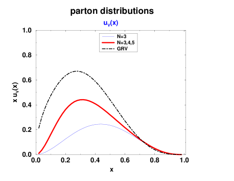
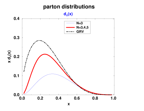
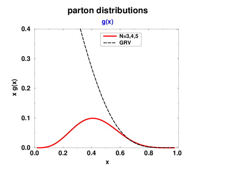
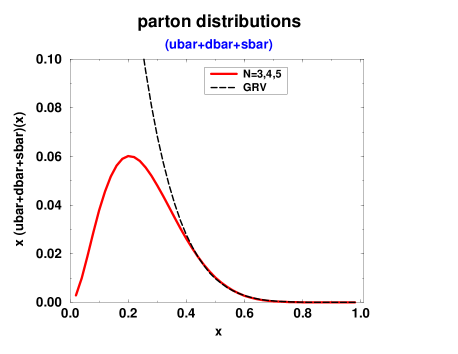
Figure 3: Parton distributions obtained from the $N=3,4,5$ Fock states ($P_{3}=0.17$, $P_{4}=P_{5}=0.1$). The model results are compared to the 1995 GRV LO parametrisation [28] at a factorisation scale of 1 GeV. For the sea distributions we sum over the three flavours.

The spin dependent parton distributions allow another interesting test of our approach. These distributions measure the difference between the distributions of type-$a$ partons with positive and negative helicity. In analogy to the unpolarised distribution discussed above we find within our model

$$\Delta{\rm q}_{a}^{(N)}(x)=\Delta b_{a}^{(N)}\,P_{N}\,x^{n_{a}}\,(1-x)^{m_{a}(N)}\,\;\left[1+\Delta c_{a}^{(N)}\,(1-x)+\Delta d_{a}^{(N)}\,(1-x)^{2}\right]$$ (64)

with the coefficients listed in Tab. 3. The powers $n_{a}$ and $m_{a}(N)$ are the same as the ones for unpolarised distributions, given by (60). As a consequence of our simple assumptions that the gluons and sea quark pairs are unpolarised we have $\Delta{\rm g}^{(4)}(x)=\Delta\overline{\rm q}^{(5)}(x)=0$. Note also that $\Delta{\rm q}_{a}^{(N)}(x)\propto{\rm q}_{a}^{(N)}(x)$ at large $x$. While the constants of proportionality are close to unity for the valence ${\rm u}$-quark distributions, they are negative or even zero for valence ${\rm d}$-quarks.

$\Delta{\rm q}_{a}^{(N)}$	$\Delta b_{a}^{(N)}$	$\Delta c_{a}^{(N)}$	$\Delta d_{a}^{(N)}$	$m_{a}(N)$
$\Delta{\rm u}_{v}^{(3)}$	$40\cdot\frac{140}{87}$	$-\frac{21}{20}$	$\frac{9}{40}$	3
$\Delta{\rm d}_{v}^{(3)}$	$-\phantom{\cdot}\;\,\frac{140}{87}$	$\phantom{-}3$	$\frac{9}{5}$	3
$\Delta{\rm u}_{v}^{(4)}$	$16\cdot\frac{990}{37}$	$-\frac{3}{2}$	$\frac{9}{16}$	7
$\Delta{\rm d}_{v}^{(4)}$	$\phantom{40\cdot}\;\,0$	$\phantom{-}0$	0	7
$\Delta{\rm u}_{v}^{(5)}$	$40\cdot\frac{264}{29}$	$-\frac{6}{5}$	$\frac{27}{80}$	7
$\Delta{\rm d}_{v}^{(5)}$	$-\phantom{\cdot}\;\,\frac{264}{29}$	$\phantom{-}\frac{3}{2}$	$\frac{1}{2}$	7

Table 3: Coefficients for the Fock state contributions to the spin-dependent parton distribution functions according to Eq. (64). The powers $m_{a}(N)$ from (60) are also given.

In Fig. 4 we compare our predictions with the parametrisation proposed in Ref. [38]. As we see, surprisingly good agreement is obtained in our simple model. There is also fair agreement with the polarised parton distributions determined in [39] at large $x$. The relative strength of $\Delta{\rm u}_{v}$ and $\Delta{\rm d}_{v}$ in that region reflects the spin structure of the valence Fock state and the asymmetry in its distribution amplitude.

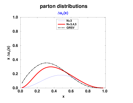
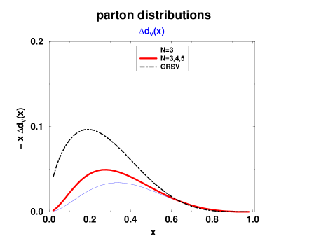
Figure 4: Spin-dependent valence quark distributions $\Delta{\rm u}_{v}$ and $\Delta{\rm d}_{v}$. The model results are compared to the parametrisation of Ref. [38].

7 Form factors

According to Drell and Yan [14] the Dirac form factor can be represented as the overlap of LCWFs as

$$F_{1}(t)\,=\,\sum_{N}\;F_{1}^{(N)}(t)$$ (65)

with individual Fock state contributions

$$F_{1}^{(N)}(t)\,=\,\sum_{a}\;e_{a}\,\sum_{j}\sum_{\beta}\int\,[{\rm d}\tilde{x}]_{N}[{\rm d}^{2}\tilde{\bf k}_{\perp}]_{N}\,\Psi^{*}_{N\beta}(\hat{x}^{\prime}_{i},{\hat{\bf k}^{\prime}_{\perp i}})\,\Psi_{N\beta}(\tilde{x}_{i},{\tilde{\bf k}_{\perp i}})\,\>,$$ (66)

where $j$ runs over all partons of type $a$. We use our symmetric frame to evaluate the overlap, the primed and unprimed arguments in (66) are therefore related by (15) and we have ${\bf\Delta}_{\perp}^{2}=-t$. Performing the ${\bf k}_{\perp}$-integrals for the $N=3,4,5$ Fock states with the help of Eq. (51), we arrive at

$$F_{1\,p}^{(N)}(t) = \int{\rm d}x\,\exp{\left[\frac{1}{2}\,a^{2}_{N}\,t\,\frac{1-x}{x}\right]}\,\left\{e_{u}\,{\rm u}_{v}^{(N)}(x)+e_{d}\,{\rm d}_{v}^{(N)}(x)\right\}\>,$$

$$F_{1\,n}^{(N)}(t) = \int{\rm d}x\,\exp{\left[\frac{1}{2}\,a^{2}_{N}\,t\,\frac{1-x}{x}\right]}\,\left\{e_{u}\,{\rm d}_{v}^{(N)}(x)+e_{d}\,{\rm u}_{v}^{(N)}(x)\right\}\>.$$ (67)

for the proton and neutron form factors. The appearance of the parton distributions here is a consequence of the fact that the integrand in their overlap representation (55) is obtained from the one in (66) by setting ${\bf\Delta}_{\perp}=0$. Thus the ${\bf k}_{\perp}$-integrals only differ by the exponential factor of (52) at $\zeta=0$, which arises from the Gaussian ${\bf k}_{\perp}$-dependence of our wave functions.

It is now suggestive to assume that the ${\bf k}_{\perp}$-dependence of all Fock state wave functions is given by the Gaussian (42) and to approximate all $a_{N}$ with a common transverse size parameter $a$. Summing over $N$ in (65) then leads to a representation of form factors in terms of the valence quark distribution functions:

$$F_{1\,p}(t) \simeq \int{\rm d}x\,\exp{\left[\frac{1}{2}\,a^{2}\,t\,\frac{1-x}{x}\right]}\,\left\{e_{u}\,{\rm u}_{v}(x)+e_{d}\,{\rm d}_{v}(x)\right\}\>,$$

$$F_{1\,n}(t) \simeq \int{\rm d}x\,\exp{\left[\frac{1}{2}\,a^{2}\,t\,\frac{1-x}{x}\right]}\,\left\{e_{u}\,{\rm d}_{v}(x)+e_{d}\,{\rm u}_{v}(x)\right\}\>,$$ (68)

a formula recently proposed by Radyushkin [17]. Remarkably, inclusive observables are related to exclusive ones. The chief advantage of this formula is its independence from any explicit form of the distribution amplitudes. Of course a common value for the transverse size parameter for all Fock states is unrealistic: as we saw before the valence Fock state is rather compact corresponding to about a half of the charge radius. Consequently the higher Fock states have to develop the full radius. For the purpose of evaluating the form factors from Eqs. (65) and (67) we take $a_{3}=a_{4}=a_{5}$ as before and put as a simple ansatz $a_{N}=1.3\,a_{3}$ for $N>5$, where the factor 1.3 is adjusted to the data for $F_{1\,p}$. A substantially larger factor would strongly suppress the higher Fock state contributions, a smaller one would lead to large contributions exceeding the form factor data. Then we set

$$\sum_{N>5}\,q_{a}^{(N)}(x)=\,q_{a}(x)-\sum_{N=3,4,5}\,q_{a}^{(N)}(x)\>,$$ (69)

where ${\rm q}_{a}$ is taken from the GRV parametrisation [28] and the three lowest Fock state contributions from our model. In this way we account for the sum of all Fock states in a phenomenological way. The results obtained in this manner are confronted to the data [40, 41] in Fig. 5.

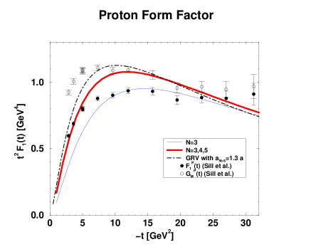
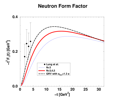
Figure 5: Electromagnetic form factor of the proton and neutron using the model parton distributions for the valence Fock state only, the $N=3,4,5$ Fock states, and all Fock states on the basis of the GRV parametrisation at the factorisation scale 1 GeV [28], cf. (69). Data for $F_{1}$ and $G_{M}$ are taken from [40, 41].

For large values of the momentum transfer our simple model agrees very well with the data, i.e. the dimensional counting behaviour is well mimicked by soft physics. Below about $10\,\,{\rm GeV}^{2}$ the model is not perfect, deviations of the order of 20$\%$, i.e. of the order of $m^{2}/(-t)$, are to be noticed. Such corrections are to be expected in our model, where proton spin-flip effects and orbital angular momentum in the wave functions are not taken into account as we discussed in see Sect. 4.2. In reality spin flip effects are not very small as is indicated by the difference between the Dirac and magnetic form factors, $F_{1}$ and $G_{M}$, see Fig. 5. In view of these approximations we are satisfied with our results even in the range $5\,\,{\rm GeV}^{2}<-t<10\,\,{\rm GeV}^{2}$. We observe from Fig. 5 the dominance of the valence Fock state contributions. For $-t>10\,\,{\rm GeV}^{2}$ all other Fock states contribute less than 20$\%$; each individual Fock state provides only a small correction to the form factor. This can be regarded as a justification of the rough treatment of the $N=4$ and 5 Fock states introduced in Sect. 5. We also remark that the parameters $f_{3}$ and $a_{3}$ of (43) used in this work have been obtained in [16] by requiring that the data for $F_{1\,p}$ be saturated by the soft overlap of the valence Fock state only. Given the uncertainties just discussed and our simplified treatment of the higher Fock states we think however that readjusting these parameters is not necessary here. As for the neutron form factor, we mentioned in Sect. 6 that totally symmetric wave functions lead to the relation ${\rm u}_{v}^{(N)}(x)=2{\rm d}_{v}^{(N)}(x)$, which according to Eq. (67) would lead to a vanishing contribution to $F_{1\,n}$. Hence the asymmetries in the LCWFs generate the neutron form factor.

For wave functions of the type we are considering here the leading powers $m_{q}(N)$ of $(1-x)$ in the valence distributions ${\rm q}_{v}^{(N)}(x)$ correspond to leading powers $m_{q}(N)+1$ of $1/t$ in the asymptotic behaviour of the corresponding Fock state contribution to $F_{1}(t)$. Hence for sufficiently large $-t$ the valence Fock state dominates the form factor with only small corrections from the next Fock states. It is important to realise that this asymptotic behaviour of the overlap contributions does not set in before $-t\simeq 100\,\,{\rm GeV}^{2}$ since the expansion of the integrals appearing in (67) into a power series in $1/t$ converges very slowly. We remark that the dominance of the soft overlap contribution is consistent with the strength of the perturbative contribution to the proton form factor, which drops as $1/t^{2}$. As reported in Ref. [16] the perturbative contribution evaluated from our valence Fock state wave function can be neglected for experimentally accessible momentum transfers. For $-t$ larger than about $500$ GeV², however, the perturbative contribution will dominate since our overlap contribution asymptotically behaves as $1/t^{4}$.

In analogy to the electromagnetic case we can also calculate the charged current axial form factor of the nucleon. The various contributions are now weighted by the quark helicities and isospin, leading to

$$F_{A} = \sum_{N}\int{\rm d}x\,\exp{\left[\frac{1}{2}\,a_{N}^{2}\,t\,\frac{1-x}{x}\right]}$$ (71)

$$\quad\times\,\left\{\Delta{\rm u}_{v}^{(N)}(x)+2\,\Delta\overline{\rm u}^{(N)}(x)-\Delta{\rm d}_{v}^{(N)}(x)-2\,\Delta\overline{\rm d}{}^{(N)}(x)\right\}\>,$$

Evaluating the axial form factor along the lines described for the electromagnetic case we find fair agreement with the dipole parametrisation of the admittedly low-$t$ neutrino data [42].

8 Large angle Compton scattering

Using our expressions (29), (4.1) for the handbag amplitude and neglecting the contribution from the proton spin flip form factor $R_{T}$, we obtain the cross section for real Compton scattering with unpolarised photons and protons as

$$\frac{{\rm d}\sigma}{{\rm d}t}=\frac{2\pi\alpha_{\it em}^{2}}{s^{2}}\,\left[-\frac{u}{s}-\frac{s}{u}\right]\,\left\{\frac{1}{2}\,\left(R_{V}^{2}(t)+R_{A}^{2}(t)\right)-\frac{us}{s^{2}+u^{2}}\,\left(R_{V}^{2}(t)-R_{A}^{2}(t)\right)\right\}\,.$$ (72)

As explained in Sect. 3.1.2 we can also calculate the Compton amplitude as an overlap of LCWFs in the symmetric frame of Sect. 2.2. Using the same approximations as in the handbag calculation, Sect. 4.1, and comparing with (29), (4.1) we obtain the analogues of the Drell-Yan formula (65), (66) for our form factors $R_{V}$ and $R_{A}$. With our Gaussian ansatz (42) for the ${\bf k}_{\perp}$-dependence of the LCWFs and the integral (50) the form factors $R_{V}$ and $R_{A}$ can then be written as

$$R_{V}(t) = \sum_{N}\;\int\frac{{\rm d}x}{x}\exp{\left[\frac{1}{2}\,a^{2}_{N}\,t\,\frac{1-x}{x}\right]}\;\left\{\,e_{u}^{2}\;[{\rm u}_{v}^{(N)}(x)+2\,\overline{\rm u}^{(N)}(x)]\right.$$

$$\hskip 60.00009pt\left.{}+e_{d}^{2}\;[{\rm d}_{v}^{(N)}(x)+2\,\overline{\rm d}{}^{(N)}(x)]+e_{s}^{2}\;2\,\overline{\rm s}{}^{(N)}(x)\right\}\>,$$

$$R_{A}(t) = \sum_{N}\;\int\frac{{\rm d}x}{x}\exp{\left[\frac{1}{2}\,a^{2}_{N}\,t\,\frac{1-x}{x}\right]}\;\left\{\,e_{u}^{2}\;[\Delta{\rm u}_{v}^{(N)}(x)+2\,\Delta\overline{\rm u}^{(N)}(x)]\right.$$ (73)

$$\hskip 60.00009pt\left.{}+e_{d}^{2}\;[\Delta{\rm d}_{v}^{(N)}(x)+2\,\Delta\overline{\rm d}{}^{(N)}(x)]+e_{s}^{2}\;2\,\Delta\overline{\rm s}{}^{(N)}(x)\right\}\>,$$

in close analogy to the expressions (67) for the Dirac form factor $F_{1}$. Our numerical predictions for $R_{V}$ and $R_{A}$ are shown in Fig. 6.

If one makes the assumption that $R_{A}=R_{V}$ as was done in [17] then one obtains the suggestive result that the cross section for Compton scattering on the proton is just given by the familiar Klein-Nishina expression for Compton scattering on a free quark times the square of the form factor $R_{V}(t)$, which describes the target structure. In our model the ratio of $R_{A}$ and $R_{V}$ is however rather far from 1 for the values of $-t$ we consider, cf. Fig. 6. From (73) one sees that $R_{A}\approx R_{V}$ would require all quarks and antiquarks to be completely polarised along the proton spin, i.e. ${\rm q}_{a}^{(N)}(x)\approx\Delta{\rm q}_{a}^{(N)}(x)$ for all $N$ and $a$, in the range of $x$ dominating the integrals. For ${\rm u}$-quarks this holds indeed if $x$ is close to 1, but not for the intermediate $x$ that are important at our values of $-t$, while for ${\rm d}$-quarks the unpolarised and polarised quark distributions even have opposite sign. We therefore keep both terms $R_{V}^{2}(t)+R_{A}^{2}(t)$ and $R_{V}^{2}(t)-R_{A}^{2}(t)$ in (72); they reflect the fact that the proton target has a nontrivial quark spin structure. Using measurements at different values of $s$ and $t$ and a Rosenbluth-type separation it will in principle be possible to isolate the new form factors $|R_{V}(t)|$ and $|R_{A}(t)|$ from sufficiently accurate experimental data, and to compare them with our predictions.

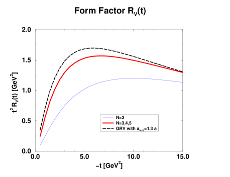
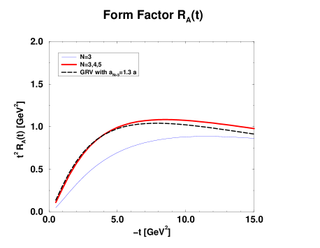
Figure 6: The form factors $R_{V}(t)$ and $R_{A}(t)$, evaluated with our model for LCWFs.

In Fig. 7 we show our results for the Compton cross section. Given the quality of the data, and the small energies and low values of $-t$ and $-u$ at which they are available, our predictions compare fairly well with experiment. As a minimum condition for our approximations discussed in Sect. 4.1 to be applicable we only take into account data points satisfying $-t,\,-u\geq 2.5\,\,{\rm GeV}^{2}$. Better data and data at larger energies are definitely required for a severe check of the new approach and its confrontation with the hard scattering mechanism. For comparison we also show predictions for the Compton cross section at a photon energy of 12  GeV that may be reached at an upgraded JLab facility [43]. At such an energy and at c.m. scattering angles around $90^{\circ}$ the kinematical conditions for the approach presented here would be satisfied. Still higher energies, perhaps accessible at ELFE [44], would be even better.

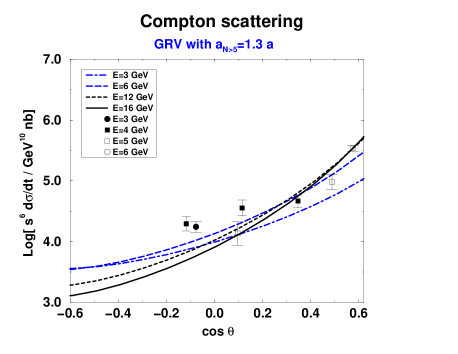
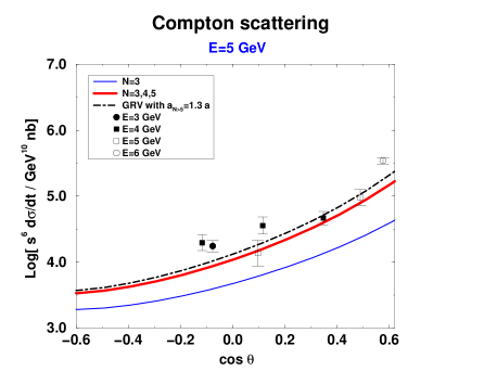
Figure 7: The Compton cross section scaled by $s^{6}$ versus $\cos{\theta}$, where $\theta$ is the scattering angle in the c.m. Data, for $-t,\,-u\geq 2.5\,\,{\rm GeV}^{2}$ only, are taken from Ref. [45]. Left: Model predictions obtained from the GRV parametrisation [28] for various photon energies in the laboratory frame. Right: Model predictions decomposed into separate Fock state contributions at a photon energy of 5 GeV.

Dimensional counting [46] predicts that the Compton cross section scaled by $s^{6}$ only depends on the ratio $t/s$ or, equivalently, on the scattering angle $\theta$ in the photon-proton c.m. From Fig. 7 one observes that the soft contributions do not exhibit this counting rule behaviour, although they are close to it. $s^{6}$-scaling holds in our approach as long as $R_{V}$ and $R_{A}$ behave as $1/t^{2}$. As one can observe from Fig. 6 this is approximately true for $-t$ in the range from about 5 to 15 GeV². For energies between, say, 3 and 6 GeV in the laboratory frame such $t$-values are only reached in the backward hemisphere. In this case the energy dependence of the scaled Compton cross section is hence much milder in the backward than in the forward hemisphere (see Fig. 7). For energies as large as for instance 12 to 15 GeV the situation is reversed. The $t$-values are so large in the backward hemisphere that $R_{V}$ and $R_{A}$ do not behave as $1/t^{2}$ any more but gradually turn into the soft physics asymptotics $1/t^{4}$. Consequently the scaled Compton cross section exhibits a stronger energy dependence in the backward hemisphere than in the forward one. For very high energies the soft physics contribution to the large angle Compton cross section scales as $s^{-10}$. We note that Radyushkin’s result [17] that all the curves for different energies intersect each other at $\cos{\theta}=-0.6$ does not hold in general. This result may depend on specific assumptions made in [17] and holds at best in a rather limited region of energy. It is an goal of utmost importance to test the energy dependence of the Compton cross section experimentally in the relevant kinematical region $s,-t,-u\gg m^{2}$. The present data are neither accurate enough nor really satisfy the kinematical requirements.

The Compton cross section has also been calculated within perturbative QCD [47] and within a diquark model [27] that combines perturbative elements with additional soft physics (correlations in the proton wave function modelled as diquarks). Both models can also account for the data although, as we said before, the quality of the data is insufficient for a severe test of the models. The diquark model does not lead to the dimensional counting behaviour either; it turns out that the energy dependence of the scaled cross section in the forward and backward hemisphere predicted by that model is opposite to the one of the approach proposed here and shown in Fig. 7.

In the leading twist hard scattering calculation of [47] proton distribution amplitudes are employed which are strongly concentrated in the end point regions, and thus differ drastically from the one determined in Ref. [16] and used here (cf. Eq. (41)). For such distribution amplitudes the perturbative analysis of Compton scattering, quite like that of the nucleon form factor [8], may be afflicted by large contributions from the soft end point regions, where perturbative QCD is not applicable as we mentioned in the introduction. We emphasise that in the perturbative approach the dimensional counting rule behaviour of the Compton cross section is modified by powers of $\log{s}$ arising from running of the the strong coupling constant $\alpha_{s}$ ($d\sigma/dt\propto\alpha_{s}^{4}$) and from the evolution of the proton wave function. These effects have not been taken into account as yet. It remains to be seen how much these $\log$s will change the results quoted in Ref. [47]. One may also expect that the inclusion of transverse momentum effects and Sudakov suppressions in the perturbative analysis leads to a similarly strong reduction of the Compton amplitude as was found for the proton form factor [12]. In view of this it seems premature to us to claim a success of the purely perturbative approach in Compton scattering.

9 Skewed parton distributions

In this section we are going to investigate skewed parton distributions (SPDs) [3, 48]. These distributions are the non-perturbative input for Compton scattering in the deep virtual region of small $-t$ but large $Q^{2}$ and $s$. Factorisation of the process into hard and soft physics [3, 23] assures that, like the usual parton distributions, the SPDs are universal in the sense that they occur in different hard processes, e.g. in hard meson production.

As explained in Sect. 3.1.2 we will restrict our investigation of SPDs to the kinematical region where they describe how a parton with momentum $k$ is taken out from the proton with momentum $p$ and, having undergone a hard scattering, inserted back with momentum $k+\Delta$ as a parton inside the scattered proton with momentum $p+\Delta$ (see Fig. 1(b)). Due to this restriction we are unable to calculate the full amplitude of the deep virtual Compton scattering process, which includes the region $0<x<\zeta$ where we do not have a simple representation of SPDs as an overlap of LCWFs. In a restricted kinematical region, however, we are able to calculate the process independent SPDs, which are of interest in their own. We will also be able to check whether they behave correctly in the formal forward limit $\Delta=0$, and whether they satisfy bounds coming from positivity requirements [49, 50, 51].

To date essentially nothing is known experimentally about skewed distributions. However, various model estimates of the SPDs have been made recently: for instance a bag model calculation [52], a chiral quark-soliton model [53], and a scalar toy model [3]. A number of simple ansätze has also been proposed [51, 54]. In particular the question whether there is a strong dependence on the skewedness parameter $\zeta$ is being debated.

The spin independent skewed distributions are defined by

$$p^{+}\,\int\frac{dz^{-}}{2\pi}\;e^{ixp^{+}z^{-}}\;\langle p^{\prime}|\overline{\psi}_{a}(0)\,\gamma^{+}\,\psi_{a}(z^{-})|p\rangle=\widetilde{{\cal F}}_{\zeta}^{\,a}(x;t)\;\bar{u}(p^{\prime})\,\gamma^{+}\,u(p)+\mbox{``$\widetilde{{\cal K}}$-term''}\>,$$ (74)

where here and in the following $a$ denotes a quark flavour, antiquarks being explicitly labelled by $\overline{a}$. The $\widetilde{{\cal K}}$-term in (74) goes with the tensor current of the proton and is related to proton helicity flip. Like the Pauli form factor $F_{2}$ and our form factor $R_{T}$ we cannot evaluate it in our model as explained in Sect. 4.2. In the definition (74) we follow the conventions of Radyushkin for nonforward distributions, cf. Eqs. (9.1) and (9.2) of [3]. The kinematical variables $x$ and $\zeta$ turn out to be most convenient for calculating the overlap of LCWFs. The relation to Ji’s original definition of off-forward distributions, where a different choice of variables is made, can be found in Ref. [3], Eqs. (9.6) and (9.7), and in Ref. [48] Eqs. (24) and (25).

The matrix element in (74) is nonzero in the range $-1+\zeta<x<1$, cf. [3, 25, 48]. Re-interpreting a quark with negative momentum fraction as an antiquark with positive fraction one finds that $-1+\zeta<x<0$ describes the emission and absorption of an antiquark, just as $\zeta<x<1$ does for a quark, while in the region $0<x<\zeta$ the proton $p$ emits a quark-antiquark pair and is left as a proton with momentum $p+\Delta$.

The definition (74) reveals the close relationship of SPDs with the usual quark distributions and with the Dirac form factor. Indeed one finds the reduction formulas

$$\widetilde{{\cal F}}_{\zeta=0}^{\,a}(x;t=0)={\rm q}_{a}(x)$$ (75)

and

$$\sum_{a}e_{a}\int_{-1+\zeta}^{1}\widetilde{{\cal F}}_{\zeta}^{\,a}(x;t)\;{\rm d}x=F_{1}(t)\>.$$ (76)

Eq. (75) can be explicitly checked in our results, while we cannot evaluate the moments in (76), which contain the region $0<x<\zeta$ we do not model here, except in the case $\zeta=0$.

We now turn to the derivation of an overlap formula for the SPDs. In close analogy to the steps that lead to Eq. (28) the amplitude for DVCS can be written in terms of proton matrix elements as

$${\cal A} = \sum_{a}(ee_{a})^{2}\int_{-1+\zeta}^{1}\frac{{\rm d}x}{2\sqrt{|xx^{\prime}|}}\,\sum_{\lambda}\,\int{{\rm d}z^{-}\over 2\pi}\,e^{i\,xp^{+}z^{-}}\,\langle p^{\prime}|\,\overline{\psi}{}_{a}(0)\,\gamma^{+}\frac{1+\lambda\gamma_{5}}{2}\,\psi_{a}(z^{-})\,|p\rangle$$ (77)

$$\times\left[\theta(\zeta<x<1)\,\bar{u}(\bar{k}^{\prime},\lambda)H(\bar{k}^{\prime},\bar{k})u(\bar{k},\lambda)\,\right.$$

$$\left.{}-\theta(0<x<\zeta)\,\bar{v}(-\bar{k}^{\prime},-\lambda)H(\bar{k}^{\prime},\bar{k})u(\bar{k},\lambda)\,\right.$$

$$\left.{}+\theta(-1+\zeta<x<0)\,\bar{v}(-\bar{k}^{\prime},-\lambda)H(\bar{k}^{\prime},\bar{k})v(-\bar{k},-\lambda)\,\right]\>,$$

with the conventions for spinors given before Eq. (27). The different kinematical regions mentioned above can easily be recognised. The hard scattering is now approximated as collinear, neglecting $-t$ and $m^{2}$ compared with $Q^{2}$ and setting $\bar{k}=[xp^{+},0,{\bf 0}_{\perp}]$, $\bar{k}^{\prime}=[x^{\prime}p^{+},0,{\bf 0}_{\perp}]$. On the other hand, direct calculation of the overlap diagrams starting from the Fock state decomposition of the proton (cf. Sect. 5) gives the contribution of the region $\zeta<x<1$ to the amplitude as

$${\cal A}^{\prime} = \sum_{a}(ee_{a})^{2}\,\int_{\zeta}^{1}{\rm d}x\,\sum_{N}\sum_{j}\sum_{\beta}\;\int[{\rm d}x]_{N}[{\rm d}^{2}{\bf k}_{\perp}]_{N}\;\delta(x-x_{j})\frac{1}{\sqrt{x_{j}x_{j}^{\prime}}}\,\left(1-\zeta\right)^{1-{N\over 2}}$$ (78)

$$\times\,\Psi^{*}_{N\beta}(\breve{x}^{\prime}_{i},\breve{\bf k}^{\prime}_{\perp i})\,\Psi_{N\beta}(x_{i},{\bf k}_{\perp i})\;\bar{u}(\bar{k}^{\prime},\lambda)H(\bar{k}^{\prime},\bar{k})u(\bar{k},\lambda)\>,$$

where $j$ runs over quarks of flavour $a$. Note that the label $\beta$ includes a dependence on the parton spin $\lambda$. The arguments of the outgoing wave function $\breve{x}^{\prime}_{i}$ and $\breve{\bf k}^{\prime}_{\perp i}$ are related to $x_{i}$ and ${\bf k}_{\perp i}$ by (2.4). From the comparison of (78) with (77) and the definition (74) we obtain the overlap formula for spin-independent SPDs in the region $\zeta<x<1$:

$$\widetilde{{\cal F}}_{\zeta}^{\,a\,(N)}(x;t)\,=\,\left(1-\zeta\right)^{{1-N}\over 2}\,\sum_{j}\sum_{\beta}\;\int[{\rm d}x]_{N}[{\rm d}^{2}{\bf k}_{\perp}]_{N}\;\delta(x-x_{j})\;\Psi^{*}_{N\beta}(\breve{x}^{\prime}_{i},\breve{\bf k}^{\prime}_{\perp i})\,\Psi_{N\beta}(x_{i},{\bf k}_{\perp i})$$ (79)

with $j$ again running over all quarks of flavour $a$. Comparing with (55) we see that the boundary condition (75) is correctly implemented in our approach. As for the sum rule (76) we find with (15) and (2.4) that in the case $\zeta=0$ the overlap expression (79) and the corresponding contribution from antiquarks reproduce the Drell-Yan formula (65).

We notice that for $\zeta<x<1$ the r.h.s of (79) has the structure of a scalar product in the Hilbert space of wave functions $\Psi_{N\beta}(x_{i},{\bf k}_{\perp i})$. Writing down the Cauchy-Schwarz inequality for (79) and using the reduction formula (75) we find

$$\left|\,\widetilde{{\cal F}}_{\zeta}^{\,a\,(N)}(x;t)\,\right|\leq\frac{1}{\sqrt{1-\zeta}}\;\sqrt{{\rm q}_{a}^{(N)}(x)\;{\rm q}_{a}^{(N)}\left({\textstyle\frac{x-\zeta}{1-\zeta}}\right)}$$ (80)

for the contribution of each Fock state. Notice that at the points $x=\zeta$ and $x=1$ both sides of (80) are zero because in the corresponding overlap integrals there are wave functions taken at their end points. Summing (79) over all Fock states one obtains the analogue of (80) for the complete distributions; it is precisely the positivity constraint on SPDs derived by Pire, Soffer and Teryaev [50], which is thus satisfied by the overlap formula (79).

To discuss the emission and reabsorption of an antiquark it is useful to define $\widetilde{{\cal F}}_{\zeta}^{\,\overline{a}}(x;t)$ by the r.h.s. of (74) with the field operators replaced with the charge conjugated ones. One easily finds the relation $\widetilde{{\cal F}}_{\zeta}^{\,\overline{a}}(x;t)=-\widetilde{{\cal F}}_{\zeta}^{\,a}(\zeta-x;t)$. In the region $\zeta<x<1$ the distribution $\widetilde{{\cal F}}_{\zeta}^{\,\overline{a}}(x;t)$ describes the emission of an antiquark with momentum fraction $x$ and its reabsorption with fraction $x^{\prime}=x-\zeta$; along the same lines as above one obtains its overlap representation as the r.h.s. of (79) with $j$ running over antiquarks instead of quarks. One then has of course the analogues of the reduction formula (75) and the bound (80) for $\widetilde{{\cal F}}_{\zeta}^{\,\overline{a}}(x;t)$ and the usual antiquark distributions.

Inserting our $N=3,4,5$ Fock state wave functions of Sect. 5 in (79) we obtain for the skewed ${\rm u}$ and ${\rm d}$ valence distributions

$$\widetilde{{\cal F}}_{\zeta}^{\,a\,(N)}(x;t)-\widetilde{{\cal F}}_{\zeta}^{\,\overline{a}\,(N)}(x;t)=b_{a}^{(N)}\;P_{N}\;(1-\zeta)^{-\frac{N+1}{2}-l_{g}}\;\Upsilon_{N}\left(x,\zeta;-t\,(1-\zeta)-\zeta^{2}m^{2}\right)$$ (81)

$$\times\,x^{n_{a}}(1-x)^{m_{a}(N)}\;\left[(1-\zeta)+c_{a}^{(N)}\,\left(1-\frac{\zeta}{2}\right)(1-x)+d_{a}^{(N)}\,(1-x)^{2}\right]\>,$$

where we remember the expression (52)

$$\Upsilon_{N}(x,\zeta;{\bf\Delta}_{\perp}^{2})=\left(\frac{2}{2-\zeta}\right)^{N-2}\frac{2(x-\zeta)}{(x-\zeta)+x(1-\zeta)^{2}}\;\exp\left[\frac{-\,a_{N}^{2}\,{\bf\Delta}_{\perp}^{2}\,(1-x)}{(x-\zeta)+x(1-\zeta)^{2}}\right]$$

given at the end of Sect. 5 and make use of the relation (10) between ${\bf\Delta}_{\perp}^{2}$, $t$ and $\zeta$. The exponents $n_{a}$, $m_{a}(N)$ and the coefficients $b_{a}^{(N)}$, $c_{a}^{(N)}$ and $d_{a}^{(N)}$ are the same as for the valence quark distributions discussed in Sect. 6, cf. Eq. (60) and Tab. 2, and $l_{g}$ is the number of gluons in the corresponding Fock state. For $\zeta=0$ our result (81) simplifies to

$$\widetilde{{\cal F}}_{\zeta=0}^{\,a\,(N)}(x;t)-\widetilde{{\cal F}}_{\zeta=0}^{\,\overline{a}\,(N)}(x;t)=\left({\rm q}_{a}^{(N)}(x)-\overline{\rm q}_{a}^{(N)}(x)\right)\,\exp{\left[\frac{1}{2}\,a^{2}_{N}\,t\,\frac{1-x}{x}\right]}\>,$$ (82)

which is the origin of our simple representations (67) and (73) of form factors. Finally we find that with our wave functions the skewed antiquark and ${\rm s}$-quark distributions are related with the ${\rm d}$ valence distribution by the analogues of Eqs. (58) and (59).

In Fig. 8 we display our results (81) summed over the $N=3,4,5$ Fock states for fixed $t$-values of $-0.5\,{\rm GeV}^{2}$ and $-1.5\,{\rm GeV}^{2}$. We remember from the end of Sect. 2.1 that $-t\geq\zeta^{2}m^{2}/(1-\zeta)$. At fixed $t$ this imposes $\zeta\leq\zeta_{\it max}$ with

$$\zeta_{\it max}=\frac{\sqrt{t\,(t-4m^{2})}+t}{2m^{2}}\>.$$ (83)

We remark at this point that the $t$-dependence of the SPDs residing in the factor $\Upsilon_{N}$ does not factorise in our approach but mixes with the dependence on $x$ and $\zeta$ in the exponent of (52); note that the transverse momenta $\breve{\bf k}^{\prime}_{\perp i}$ in the overlap formula (79) implicitly depend on $x$, $\zeta$ and ${\bf\Delta}_{\perp}$ through (2.4). A significant dependence on the skewedness parameter $\zeta$ shows up in our results; a fact which is not surprising since $\zeta$ determines the momentum fraction of the active parton in the light-cone wave function of the outgoing nucleon.

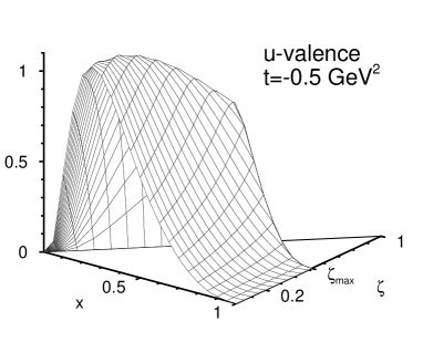
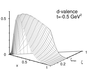
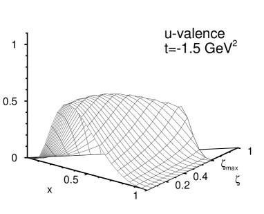
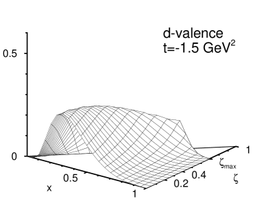
Figure 8: Skewed parton distributions for ${\rm u}$ and ${\rm d}$ valence quarks in the region $\zeta<x<1$, obtained from the $N=3,4,5$ Fock states ($P_{3}=0.17$, $P_{4}=P_{5}=0.1$). The values of $\zeta_{\it max}$ are 0.52 at $t=-0.5\,{\rm GeV}^{2}$ and 0.71 at $t=-1.5\,{\rm GeV}^{2}$.

In Fig. 9 we plot the skewed ${\rm u}$ valence distributions at fixed $t$ and $\zeta$ as a function of $x$, comparing the contribution from the $N=3$ Fock state with the result summed over $N=3,4,5$. As for the usual parton distributions we see how higher Fock states become more and more important as $x$ decreases. We notice that the values of $x$ where this happens increase somewhat with $\zeta$; this can be understood from the fact that at a given $x$ the momentum fraction of the parton going back into the proton decreases with $\zeta$. The area under a curve in Fig. 9 gives the ${\rm u}$-quark contribution of the regions $-1+\zeta<x<0$ and $\zeta<x<1$ to the form factor sum rule (76). We can see that higher Fock states become less important as $-t$ increases, in agreement with what we have found for $F_{1}(t)$ in Sect. 7.

For the usual parton distributions we know that both ${\rm q}_{v}(x)$ and $\overline{\rm q}(x)$ become singular for $x\to 0$, which cannot be obtained from any finite number of Fock state contributions, all of which vanish at $x=0$. The question what the situation is for $x\to\zeta$ in skewed distributions, when the momentum fraction $x^{\prime}$ becomes zero while $x$ remains finite, cannot be answered in the framework of this paper. We therefore do not claim that our results for the contribution of the first tree Fock states describe the full distribution as $x$ comes close to $\zeta$.

Figure 9: Skewed valence ${\rm u}$-quark parton distributions in the region $\zeta<x<1$ as a function of $x$ at fixed $\zeta$ and $t$. Full lines show the sum of contributions from the $N=3,4,5$ Fock states and dashed ones the contribution from the $N=3$ Fock state alone. The vertical lines in the plots indicate the value of $x$ where the $N=3$ contribution is 80% of the one summed over $N=3,4,5$.

The definition of spin dependent SPDs is obtained from (74) by the replacements $\gamma^{+}\to\gamma^{+}\gamma_{5}$ and $\widetilde{{\cal F}}^{\,a}_{\zeta}\to\widetilde{{\cal G}}^{\,a}_{\zeta}$; for antiquarks one has $\widetilde{{\cal G}}^{\,\overline{a}}_{\zeta}(x;t)=\widetilde{{\cal G}}^{\,a}_{\zeta}(\zeta-x;t)$. The analogue of the $\widetilde{{\cal K}}$-term goes now with the pseudoscalar current of the proton and is again related to proton spin flip. From the appropriate overlap formulae we find the spin dependent skewed valence distributions

$$\widetilde{{\cal G}}_{\zeta}^{\,a\,(N)}(x;t)-\widetilde{{\cal G}}_{\zeta}^{\,\overline{a}\,(N)}(x;t)=\Delta b_{a}^{(N)}\;P_{N}\;(1-\zeta)^{-\frac{N+1}{2}-l_{g}}\;\Upsilon_{N}\left(x,\zeta;-t\,(1-\zeta)-\zeta^{2}m^{2}\right)$$ (84)

$$\times\,x^{n_{a}}(1-x)^{m_{a}(N)}\;\left[(1-\zeta)+\Delta c_{a}^{(N)}\,\left(1-\frac{\zeta}{2}\right)(1-x)+\Delta d_{a}^{(N)}\,(1-x)^{2}\right]\>,$$

where the coefficients $\Delta b_{a}^{(N)}$, $\Delta c_{a}^{(N)}$, and $\Delta d_{a}^{(N)}$ are the same as the ones for the spin dependent valence distributions listed in Tab. 3. Evidently the spin dependent skewed distributions reduce correctly to the usual ones in the limit $\zeta\to 0$ and $t\to 0$.

10 Summary

In the present paper we have linked ordinary and skewed parton distributions to soft overlap contributions to elastic form factors and to large angle Compton scattering using nucleon light-cone wave functions.

We have investigated how and under which conditions overlap contributions to exclusive processes can be expressed in terms of LCWFs. For large angle Compton scattering, at large values of the Mandelstam invariants $s$, $-t$ and $-u$, we can calculate the soft overlap contribution using its factorisation into handbag diagrams, i.e. into soft parton emission and reabsorption by the nucleon and a hard parton-photon scattering. In the case of deeply virtual Compton scattering, with large $Q^{2}$ and $s$ but small $-t$, where we cannot express the amplitude as an overlap of soft LCWFs, we have calculated the skewed parton distributions in the large-$x$ region.

For the LCWF of the three-quark nucleon Fock state we have taken over the parametrisation of [16], which involves only two parameters adjusted to data. For the Fock states with an additional gluon or quark-antiquark pair we have taken a very simple ansatz, introducing only two more parameters, which are fitted to the gluon and sea quark parton distributions from the GRV analysis [28]. The values of all four parameters come out in a range compatible with their physical meaning of Fock state probabilities or a transverse size parameter. In the overlap contributions to Compton scattering and the form factor we also estimate the net effect of all higher Fock states, using as input the difference between the GRV parton distributions and those calculated from the three lowest Fock states only.

The phenomenology we can do with our ansatz is very rich: we reproduce well the unpolarised and polarised parton distributions down to $x$ around 0.5, as well as the data for the nucleon Dirac form factors and for real Compton scattering at large c.m. angles. The inclusion of higher Fock states in the soft overlap contributions confirms that as $-t$ increases the lowest Fock states become increasingly dominant and gives an impression of the accuracy one can hope for by only taking into account the three quark state. The LCWF of [16] was constructed so as to saturate the elastic form factor data. The fact that with the same wave function one obtains a reasonable description of Compton scattering supports the hypothesis that there is no sizeable perturbative contribution to either process in the range of momentum transfers where data exist; soft physics seems to dominate as was occasionally suggested in the literature [7, 8, 10].

We stress that from the apparent agreement of exclusive data with dimensional counting rules the dominance of perturbative QCD contributions cannot be deduced. Soft physics, as for instance the overlap-type contributions which we propose, provides broad maxima in scaled observables such as $t^{2}F_{1}(t)$ and the scaled Compton cross section $s^{6}\,{\rm d}\sigma/{\rm d}t$, and thus mimics dimensional counting rule behaviour in a certain range of $t$.

Compared with the elastic form factors large angle Compton scattering has a second independent kinematical variable and thus provides an additional handle to experimentally test how well dimensional counting rules are satisfied. We further suggest that the imaginary part of the scattering amplitude, which is accessible in virtual Compton scattering with a polarised lepton beam, offers a sensible tool to investigate which dynamical mechanism is at work: in the handbag mechanism imaginary parts are only generated through loop corrections to the photon-parton subprocess, whereas in the hard scattering mechanism real and imaginary parts generically are of the same order of magnitude. Spin observables may also be sensitive probes of the underlying physics, given the particular helicity structure of the photon-parton scattering in the handbag diagrams. In any case we see a strong motivation to have further and more accurate Compton data at sufficiently high values of energy and momentum transfer.

References

- [1] D. Müller, D. Robaschik, B. Geyer, F.-M. Dittes and J. Hořejši, Fortschr. Physik 42, 101 (1994), hep-ph/9812448.
- [2] X. Ji, Phys. Rev. Lett. 78, 610 (1997); Phys. Rev. D55, 7114 (1997).
- [3] A.V. Radyushkin, Phys. Rev. D56, 5524 (1997).
- [4] G.P. Lepage and S.J. Brodsky, Phys. Rev. D22, 2157 (1980).
-
[5]
G.P. Lepage, S.J. Brodsky, T. Huang and P.B. Mackenzie,
in: Banff Summer Institute 1981, Particles
and Fields 2, eds. A.Z. Capri and A.N. Kamal (Plenum
Press, New York 1983), p. 83;
S.J. Brodsky, T. Huang and G.P. Lepage, ibid. , p. 143. - [6] V.L. Chernyak, A. Ogloblin and I.R. Zhitnitsky, Z. Phys. C42, 569 (1989).
- [7] A.V. Radyushkin, Nucl. Phys. A532, 141c (1991).
- [8] N. Isgur and C.H. Llewellyn Smith, Nucl. Phys. B317, 526 (1989).
- [9] CLEO collaboration, J. Gronberg et al., Phys. Rev. D57, 33 (1998).
-
[10]
R. Jakob, P. Kroll and M. Raulfs,
J. Phys. G22, 45 (1996);
P. Kroll and M. Raulfs, Phys. Lett. B387, 848 (1996). - [11] I.V. Musatov and A.V. Radyushkin, Phys. Rev. D56, 2713 (1997).
- [12] J. Bolz, R. Jakob, P. Kroll, M. Bergmann and N.G. Stefanis, Z. Phys. C66, 267 (1995).
-
[13]
J. Botts and G. Sterman,
Nucl. Phys. B325, 62 (1989);
H.-n. Li and G. Sterman Nucl. Phys. B381, 129 (1992). - [14] S.D. Drell and T.-M. Yan, Phys. Rev. Lett. 24, 181 (1970).
- [15] A. Schäfer, L. Mankiewicz and Z. Dziembowski, Phys. Lett. B233, 217 (1989).
-
[16]
J. Bolz and P. Kroll,
Z. Phys. A356, 327 (1996);
see also J. Bolz, doctoral thesis 1995, Wuppertal internal report WUB-DIS 95-10 (in German). - [17] A.V. Radyushkin, hep-ph/9803316.
- [18] S.J. Brodsky and G.P. Lepage, in: Perturbative Quantum Chromodynamics, ed. A. Mueller (World Scientific, Singapore 1989).
- [19] M. Sawicki, Phys. Rev. D46, 474 (1992).
- [20] M. Sawicki, Phys. Rev. D44, 433 (1991).
- [21] S.J. Brodsky and D.S. Hwang, hep-ph/9806358.
- [22] M. Burkardt, Phys. Rev. D52, 3841 (1995).
-
[23]
X. Ji and J. Osborne, Phys. Rev. D58, 094018
(1998);
J.C. Collins and A. Freund, hep-ph/9801262. - [24] J.C. Collins, L. Frankfurt and M. Strikman, Phys. Rev. D56, 2982 (1997).
- [25] M. Diehl and T. Gousset, Phys. Lett. B428, 359, (1998).
- [26] S.J. Brodsky and G.P. Lepage, Phys. Rev. D24, 2848 (1981).
- [27] P. Kroll, M. Schürmann and P.A.M. Guichon, Nucl. Phys. A598, 435 (1996).
- [28] M. Glück, E. Reya and A. Vogt, Z. Phys. C67, 433 (1995); Eur. Phys. J. C5, 461 (1998).
- [29] M.G. Sotiropoulos and G. Sterman, Nucl. Phys. B425, 489 (1994).
- [30] Z. Dziembowski, Phys. Rev. D37, 768 (1988).
- [31] B. Chibisov and A.R. Zhitnitsky, Phys. Rev. D52, 5273 (1995).
- [32] S.J. Brodsky, hep-ph/9807212
- [33] F. Hussain, J.G. Körner and G. Thompson, Ann. Phys. (N.Y.), 206, 334 (1991).
- [34] J. Bolz, P. Kroll and J.G. Körner, Z. Phys. A350, 145 (1994).
- [35] S.J. Brodsky, M. Burkardt and I. Schmidt, Nucl. Phys. B441, 197 (1995).
- [36] A.D. Martin, R.G. Roberts, W.J. Stirling and R.S. Thorne, Eur. Phys. J. C4, 463 (1998).
- [37] A. Thomas, hep-ph/9712404.
- [38] M. Glück, E. Reya, M. Stratmann and W. Vogelsang, Phys. Rev. D53, 4775 (1996).
- [39] E. Leader, A.V. Sidorov and D.B. Stamenov, hep-ph/9807251.
- [40] A.F. Sill et al., Phys. Rev. D48, 29 (1993).
- [41] A. Lung et al., Phys. Rev. Lett. 70, 718 (1993).
- [42] T. Kitagaki et al., Phys. Rev. D28, 436 (1983).
- [43] A.M. Nathan, hep-ph/9807397.
- [44] The ELFE Project, eds. J. Arvieux and E. De Sanctis, Conference Proceedings, Vol. 44 (Italian Physical Society, Bologna 1993).
- [45] M.A. Shupe et al., Phys. Rev. D19, 1921 (1979).
-
[46]
S.J. Brodsky and G.R. Farrar,
Phys. Rev. Lett. 31, 1153 (1973);
V.A. Matveev, R.M. Muradyan and A.N. Tavkhelidze, Lett. Nouvo Cim. 7, 719 (1973). -
[47]
A. Kronfeld and B. Nižić,
Phys. Rev. D44, 3445 (1991); Erratum
Phys. Rev. D46, 2272 (1992);
M. Vanderhaeghen, P.A.M. Guichon and J. Van de Wiele, Nucl. Phys. A622, 144c (1997). - [48] X. Ji, J. Phys. G24, 1181 (1998).
- [49] A.D. Martin and M.G. Ryskin, Phys. Rev. D57, 6692 (1998).
- [50] B. Pire, J. Soffer and O. Teryaev, hep-ph/9804284.
- [51] A.V. Radyushkin, hep-ph/9805342.
- [52] X. Ji, W. Melnitchouk and X. Song, Phys. Rev. D56, 5511 (1997).
- [53] V.Yu. Petrov, P.V. Pobylitsa, M.V. Polyakov, I. Börnig, K. Goeke and C. Weiss, Phys. Rev. D57, 4325 (1998).
-
[54]
M. Vanderhaeghen, P.A.M. Guichon, M. Guidal,
Phys. Rev. Lett. 80, 5064 (1998);
L. Mankiewicz, G. Piller and T. Weigl, Eur. Phys. J. C5, 119 (1998);
A.V. Radyushkin, hep-ph/9810466.