Updated Analysis of $a_{1}$ and $a_{2}$
in Hadronic Two-body Decays of $B$ Mesons

Abstract

Using the recent experimental data of $B\to D^{(*)}(\pi,\rho)$, $B\to D^{(*)}D_{s}^{(*)}$, $B\to J/\psi K^{(*)}$ and various model calculations on form factors, we re-analyze the effective coefficients $a_{1}$ and $a_{2}$ and their ratio. QCD and electroweak penguin corrections to $a_{1}$ from $B\to D^{(*)}D_{s}^{(*)}$ and $a_{2}$ from $B\to J/\psi K^{(*)}$ are estimated. In addition to the model-dependent determination, the effective coefficient $a_{1}$ is also extracted in a model-independent way as the decay modes $B\to D^{(*)}h$ are related by factorization to the measured semileptonic distribution of $B\to D^{(*)}\ell\bar{\nu}$ at $q^{2}=m_{h}^{2}$. Moreover, this enables us to extract model-independent heavy-to-heavy form factors, for example, $F_{0}^{BD}(m_{\pi}^{2})=0.66\pm 0.06\pm 0.05$ and $A_{0}^{BD^{*}}(m_{\pi}^{2})=0.56\pm 0.03\pm 0.04$. The determination of the magnitude of $a_{2}$ from $B\to J/\psi K^{(*)}$ depends on the form factors $F_{1}^{BK}$, $A_{1,2}^{BK^{*}}$ and $V^{BK^{*}}$ at $q^{2}=m^{2}_{J/\psi}$. By requiring that $a_{2}$ be process insensitive ( i.e., the value of $a_{2}$ extracted from $J/\psi K$ and $J/\psi K^{*}$ states should be similar), as implied by the factorization hypothesis, we find that $B\to K^{(*)}$ form factors are severely constrained; they respect the relation $F_{1}^{BK}(m^{2}_{J/\psi})\approx 1.9A_{1}^{BK^{*}}(m^{2}_{J/\psi})$. Form factors $A_{2}^{BK^{*}}$ and $V^{BK^{*}}$ at $q^{2}=m^{2}_{J/\psi}$ inferred from the measurements of the longitudinal polarization fraction and the $P$–wave component in $B\to J/\psi K^{*}$ are obtained. A stringent upper limit on $a_{2}$ is derived from the current bound on $\overline{B}^{0}\to D^{0}\pi^{0}$ and it is sensitive to final-state interactions.

June 1998

I Introduction

Nonleptonic two-body decays of $B$ and $D$ mesons have been conventionally studied in the generalized factorization approach in which the decay amplitudes are approximated by the factorized hadronic matrix elements multiplied by some universal, process-independent effective coefficients $a_{i}^{\rm eff}$. Based on the generalized factorization assumption, one can catalog the decay processes into three classes. For class-I decays, the decay amplitudes, dominated by the color-allowed external $W$-emission, are proportional to $a_{1}^{\rm eff}\langle O_{1}\rangle_{\rm fact}$ where $O_{1}$ is a charged current–charged current 4-quark operator. For class-II decays, the decay amplitudes, governed by the color-suppressed internal $W$-emission, are described by $a_{2}^{\rm eff}\langle O_{2}\rangle_{\rm fact}$ with $O_{2}$ being a neutral current–neutral current 4-quark operator. The decay amplitudes of the class-III decays involve a linear combination of $a_{1}^{\rm eff}\langle O_{1}\rangle_{\rm fact}$ and $a_{2}^{\rm eff}\langle O_{2}\rangle_{\rm fact}$. If factorization works, the effective coefficients $a_{i}^{\rm eff}$ in nonleptonic $B$ or $D$ decays should be channel by channel independent. Since the factorized hadronic matrix elements $\langle O_{i}\rangle_{\rm fact}$ are renormalization scheme and scale independent, so are $a_{i}^{\rm eff}$.

What is the relation between the effective coefficients $a_{i}^{\rm eff}$ and the Wilson coefficients in the effective Hamiltonian approach ? Under the naive factorization hypothesis, one has

$$a_{1}(\mu)=c_{1}(\mu)+{1\over N_{c}}c_{2}(\mu),\qquad\quad a_{2}(\mu)=c_{2}(\mu)+{1\over N_{c}}c_{1}(\mu),$$ (1)

for decay amplitudes induced by current-current operators $O_{1,2}(\mu)$, where $c_{1,2}(\mu)$ are the corresponding Wilson coefficients. However, this naive factorization approach encounters two principal difficulties: (i) the above coefficients $a_{i}$ are scale dependent, and (ii) it fails to describe the color-suppressed class-II decay modes. For example, the predicted decay rate of $D^{0}\to\overline{K}^{0}\pi^{0}$ by naive factorization is too small compared to experiment. Two different approaches have been advocated in the past for solving the aforementioned scale problem associated with the naive factorization approximation. In the first approach, one incorporates nonfactorizable effects into the effective coefficients [1, 2, 3]:

$$a_{1}^{\rm eff}=c_{1}(\mu)+c_{2}(\mu)\left({1\over N_{c}}+\chi_{1}(\mu)\right)\,,\qquad\quad a_{2}^{\rm eff}=c_{2}(\mu)+c_{1}(\mu)\left({1\over N_{c}}+\chi_{2}(\mu)\right)\,,$$ (2)

where nonfactorizable terms are characterized by the parameters $\chi_{i}$. Considering the decay $\overline{B}^{0}\to D^{+}\pi^{-}$ as an example, $\chi_{1}$ is given by

$$\chi_{1}(\mu)=\varepsilon_{8}^{(BD,\pi)}(\mu)+{a_{1}(\mu)\over c_{2}(\mu)}\varepsilon_{1}^{(BD,\pi)}(\mu),$$ (3)

where

$$\varepsilon_{1}^{(BD,\pi)} =\frac{\langle D^{+}\pi^{-}|(\bar{c}b)_{{}_{V-A}}(\bar{d}u)_{{}_{V-A}}|\overline{B}^{0}\rangle}{\langle D^{+}|(\bar{c}b)_{{}_{V-A}}|\overline{B}^{0}\rangle\langle\pi^{-}|(\bar{d}u)_{{}_{V-A}}|0\rangle}-1\,,$$ (4)

$$\varepsilon_{8}^{(BD,\pi)} =\frac{\langle D^{+}\pi^{-}|{1\over 2}(\bar{c}\lambda^{a}b)_{{}_{V-A}}(\bar{d}\lambda^{a}u)_{{}_{V-A}}|\overline{B}^{0}\rangle}{\langle D^{+}|(\bar{c}b)_{{}_{V-A}}|\overline{B}^{0}\rangle\langle\pi^{-}|(\bar{d}u)_{{}_{V-A}}|0\rangle}\,,$$ (5)

are nonfactorizable terms originated from color signlet-singlet and octet-octet currents, respectively, $(\bar{q}_{1}q_{2})_{{}_{V-A}}\equiv\bar{q}_{1}\gamma_{\mu}(1-\gamma_{5})q_{2}$, and $(\bar{q}_{1}\lambda^{a}q_{2})_{{}_{V-A}}\equiv\bar{q}_{1}\lambda^{a}\gamma_{\mu}(1-\gamma_{5})q_{2}$. The $\mu$ dependence of the Wilson coefficients is assumed to be exactly compensated by that of $\chi_{i}(\mu)$ [4]. That is, the correct $\mu$ dependence of the matrix elements is restored by $\chi_{i}(\mu)$. In the second approach, it is postulated that the hadronic matrix element $\langle O(\mu)\rangle$ is related to the tree-level one via the relation $\langle O(\mu)\rangle=g(\mu)\langle O\rangle_{\rm tree}$ and that $g(\mu)$ is independent of the external hadron states. Explicitly,

$$c(\mu)\langle O(\mu)\rangle=c(\mu)g(\mu)\langle O\rangle_{\rm tree}\equiv c^{\rm eff}\langle O\rangle_{\rm tree}.$$ (6)

Since the tree-level matrix element $\langle O\rangle_{\rm tree}$ is renormalization scheme and scale independent, so are the effective Wilson coefficients $c_{i}^{\rm eff}$ and the effective parameters $a_{i}^{\rm eff}$ expressed by [5, 6]

$$a_{1}^{\rm eff}=c_{1}^{\rm eff}+c_{2}^{\rm eff}\left({1\over N_{c}}+\chi_{1}\right)\,,\qquad\quad a_{2}^{\rm eff}=c_{2}^{\rm eff}+c_{1}^{\rm eff}\left({1\over N_{c}}+\chi_{2}\right)\,.$$ (7)

Although naive factorization does not work in general, we still have a new factorization scheme in which the decay amplitude is expressed in terms of factorized hadronic matrix elements multiplied by the universal effective parameters $a_{1,2}^{\rm eff}$ provided that $\chi_{1,2}$ are universal (i.e. process independent) in charm or bottom decays. Contrary to the naive one, the improved factorization scheme does incorporate nonfactorizable effects in a process independent form. For example, $\chi_{1}=\chi_{2}=-{1\over 3}$ in the large-$N_{c}$ approximation of factorization. Theoretically, it is clear from Eqs. (3) and (4) that a priori the nonfactorized terms $\chi_{i}$ are not necessarily channel independent. In fact, phenomenological analyses of two-body decay data of $D$ and $B$ mesons indicate that while the generalized factorization hypothesis in general works reasonably well, the effective parameters $a_{1,2}^{\rm eff}$ do show some variation from channel to channel, especially for the weak decays of charmed mesons [1, 7]. However, in the energetic two-body $B$ decays, $\chi_{i}$ are expected to be process insensitive as supported by data [4].

The purpose of the present paper is to provide an updated analysis of the effective coefficients $a_{1}^{\rm eff}$ and $a_{2}^{\rm eff}$ from various Cabibbo-allowed two-body decays of $B$ mesons: $B\to D^{(*)}D_{s}^{(*)},\,D^{(*)}(\pi,\rho),\,J/\psi K^{(*)}$. It is known that the parameter $|a_{1}^{\rm eff}|$ can be extracted from $\overline{B}^{0}\to D^{(*)+}(\pi^{-},\rho^{-})$ and $B_{s}\to D^{(*)}D_{s}^{(*)}$, $|a_{2}^{\rm eff}|$ from $B\to J/\psi K^{(*)}$, $\overline{B}^{0}\to D^{(*)0}\pi^{0}(\rho^{0})$, and $a^{\rm eff}_{2}/a^{\rm eff}_{1}$ from $B^{-}\to D^{(*)}(\pi,\rho)$. However, the determination of $a_{1}^{\rm eff}$ and $a_{2}^{\rm eff}$ is subject to many uncertainties: decay constants, form factors and their $q^{2}$ dependence, and the quark-mixing matrix element $V_{cb}$. It is thus desirable to have an objective estimation of $a^{\rm eff}_{1,2}$. A model-independent extraction of $a_{1}$ is possible because the decay modes $B\to D^{(*)}h$ can be related by factorization to the measured semileptonic decays $B\to D^{(*)}\ell\bar{\nu}$. As a consequence, the ratio of nonleptonic to differential semileptonic decay rates measured at $q^{2}=m^{2}_{h}$ is independent of above-mentioned uncertainties. The determination of $|a_{2}^{\rm eff}|$ from $B\to J/\psi K^{(*)}$ is sensitive to the form factors $F_{1}^{BK}$, $A_{1,2}^{BK^{*}}$ and $V^{BK^{*}}$ at $q^{2}=m^{2}_{J/\psi}$. In order to accommodate the observed production ratio $R\equiv\Gamma(B\to J/\psi K^{*})/\Gamma(B\to J/\psi K)$ by generalized factorization, $a_{2}^{\rm eff}$ should be process insensitive; that is, $a_{2}^{\rm eff}$ extracted from $J/\psi K$ and $J/\psi K^{*}$ final states should be very similar. This puts a severe constraint on the form-factor models and only a few models can satisfactorily explain the production ratio $R$.

The rest of this paper is organized as follows. In Sec. II, we introduce the basic formula and the classification of the relevant decay modes which have been measured experimentally. Sec. III briefly describes various form-factor models. The results and discussions for the effective parameters $a_{1}^{\rm eff}$ and $a_{2}^{\rm eff}$ are presented in Secs. IV and V, respectively. Finally, the conclusion is given in Sec. VI.

II The basic framework

Since, as we shall see below, the decays $B\to D^{(*)}D_{s}^{(*)},~{}J/\psi K^{(*)}$ receive penguin contributions, the relevant $\Delta B=1$ effective Hamiltonian for our purposes has the form

$${\cal H}_{\rm eff} = {G_{F}\over\sqrt{2}}\Bigg{\{}V_{cb}V_{uq}^{*}\Big{[}c_{1}(\mu)O_{1}^{(uq)}(\mu)+c_{2}(\mu)O_{2}^{(uq)}(\mu)\Big{]}+V_{cb}V_{cs}^{*}\Big{[}c_{1}(\mu)O_{1}^{(cs)}(\mu)+c_{2}(\mu)O_{2}^{(cs)}(\mu)\Big{]}$$ (9)

$$-V_{tb}V_{ts}^{*}\sum^{10}_{i=3}c_{i}(\mu)O_{i}(\mu)\Bigg{\}}+{\rm h.c.},$$

where

$$O_{1}^{(uq)}=(\bar{c}b)_{{}_{V-A}}(\bar{q}u)_{{}_{V-A}},\qquad\qquad\qquad\qquad O_{2}^{(uq)}=(\bar{q}b)_{{}_{V-A}}(\bar{c}u)_{{}_{V-A}},$$ (10)

$$O_{1}^{(cs)}=(\bar{c}b)_{{}_{V-A}}(\bar{s}c)_{{}_{V-A}},\qquad\qquad\qquad\qquad~{}O_{2}^{(cs)}=(\bar{s}b)_{{}_{V-A}}(\bar{c}c)_{{}_{V-A}},$$ (11)

$$O_{3(5)}=(\bar{q}b)_{{}_{V-A}}\sum_{q^{\prime}}(\bar{q}^{\prime}q^{\prime})_{{{}_{V-A}}({{}_{V+A}})},\qquad\qquad\,O_{4(6)}=(\bar{q}_{\alpha}b_{\beta})_{{}_{V-A}}\sum_{q^{\prime}}(\bar{q}^{\prime}_{\beta}q^{\prime}_{\alpha})_{{{}_{V-A}}({{}_{V+A}})},$$ (12)

$$O_{7(9)}={3\over 2}(\bar{q}b)_{{}_{V-A}}\sum_{q^{\prime}}e_{q^{\prime}}(\bar{q}^{\prime}q^{\prime})_{{{}_{V+A}}({{}_{V-A}})},\qquad\,O_{8(10)}={3\over 2}(\bar{q}_{\alpha}b_{\beta})_{{}_{V-A}}\sum_{q^{\prime}}e_{q^{\prime}}(\bar{q}^{\prime}_{\beta}q^{\prime}_{\alpha})_{{{}_{V+A}}({{}_{V-A}})},$$ (13)

with $O_{3}$–$O_{6}$ being the QCD penguin operators and $O_{7}$–$O_{10}$ the electroweak penguin operators.

To evaluate the decay amplitudes for the processes $B\to D^{(*)}D^{(*)}_{s}$, $D^{(*)+,0}(\pi^{-},\rho^{-})$, $J/\psi K^{(*)}$, we first apply Eq. (6) to the effective Hamiltonian (9) so that the factorization approximation can be applied to the tree-level hadronic matrix elements. We also introduce the shorthand notation $X^{(BF_{1},F_{2})}$ to denote the factorized matrix element with the $F_{2}$ meson being factored out [6], for instance,

$$X^{(B^{-}D^{0},\pi^{-})} \equiv \langle\pi^{-}|(\bar{d}u)_{{}_{V-A}}|0\rangle\langle D^{0}|(\bar{c}b)_{{}_{V-A}}|B^{-}\rangle,$$ (14)

$$X^{(B^{-}\pi^{-},D^{0})} \equiv \langle D^{0}|(\bar{c}u)_{{}_{V-A}}|0\rangle\langle\pi^{-}|(\bar{d}b)_{{}_{V-A}}|B^{-}\rangle\,.$$ (15)

The results are:

• Class I: $\overline{B}_{d}^{0}\to D^{(*)+}~{}\pi^{-}(\rho^{-})$
  The decay amplitudes are given by

  $$A(\overline{B}_{d}^{0}\to D^{(*)+}\pi^{-}(\rho^{-}))=\frac{G_{F}}{\sqrt{2}}{V_{cb}V_{ud}^{*}}~{}\left[a_{1}X^{(\overline{B}^{0}D^{(*)+},\pi^{-}(\rho^{-}))}+a_{2}X^{(\overline{B}^{0},D^{(*)+}\pi^{-}(\rho^{-}))}\right],$$ (16)

  where $X^{(\overline{B},D^{(*)+}\pi^{-}(\rho^{-}))}$ is the factorized $W$-exchange contribution.

• Class I: $B^{-}\to D^{(*)0}D_{s}^{(*)-}$ and $\overline{B}_{d}^{0}\to D^{(*)+}~{}D_{s}^{(*)-}$
  The decay amplitudes are given by

  $$A(B\to D\,D_{s}) = \frac{G_{F}}{\sqrt{2}}\Bigg{\{}{V_{cb}V_{cs}^{*}}~{}a_{1}-V_{tb}V_{ts}^{*}\Big{[}a_{4}+a_{10}$$ (17)

  $$+ 2(a_{6}+a_{8}){m_{D_{s}}^{2}\over(m_{b}-m_{c})(m_{c}+m_{s})}\Big{]}\Bigg{\}}X^{(BD,D_{s})}$$ (18)

  $$\cong {G_{F}\over\sqrt{2}}{V_{cb}V_{cs}^{*}}\,\tilde{a}_{1}(B\to DD_{s})X^{(BD,D_{s})}\,,$$ (19)

  where use of $V_{tb}V_{ts}^{*}\cong-{V_{cb}V_{cs}^{*}}$ has been made and

  $$\tilde{a}_{1}(B\to D\,D_{s})=a_{1}\left(1+{a_{4}+a_{10}\over a_{1}}+2{a_{6}+a_{8}\over a_{1}}\,{m_{D_{s}}^{2}\over(m_{b}-m_{c})(m_{s}+m_{c})}\right).$$ (20)

  Likewise,

  $$\tilde{a}_{1}(B\to D^{*}D_{s}) = a_{1}\left(1+{a_{4}+a_{10}\over a_{1}}-2{a_{6}+a_{8}\over a_{1}}\,{m_{D_{s}}^{2}\over(m_{b}+m_{c})(m_{s}+m_{c})}\right),$$ (21)

  $$\tilde{a}_{1}(B\to D^{(*)}D_{s}^{*}) = a_{1}\left(1+{a_{4}+a_{10}\over a_{1}}\right).$$ (22)

  Note that the decay $B^{-}\to D^{0}D_{s}^{(*)-}$ also receives a contribution from the $W$-annihilation diagram, which is quark-mixing-angle doubly suppressed, however.

• Class II: $\overline{B}_{d}^{0}\to D^{(*)0}~{}\pi^{0}(\rho^{0})$
  The factorized decay amplitudes are given by

  $$A(\overline{B}_{d}^{0}\to D^{(*)0}\pi^{0}(\rho^{0}))=\frac{G_{F}}{\sqrt{2}}{V_{cb}V_{ud}^{*}}~{}a_{2}\left[X^{(\overline{B}^{0}\pi^{0}(\rho^{0}),D^{(*)0})}+X^{(\overline{B}^{0},D^{(*)0}\pi^{0}(\rho^{0}))}\right],$$ (23)

  where $X^{(\overline{B}^{0},D^{(*)0}\pi^{0}(\rho^{0}))}$ is the factorized $W$-exchange contribution.

• Class II: $B^{+}\to J/\psi~{}K^{(*)+}$ and $B^{0}\to J/\psi~{}K^{(*)0}$
  The decay amplitudes are given by

  $$A(B\to J/\psi~{}K^{(*)})=\frac{G_{F}}{\sqrt{2}}{V_{cb}V_{cs}^{*}}~{}\tilde{a}_{2}X^{(BK^{(*)},J/\psi)}\,,$$ (24)

  where

  $$\tilde{a}_{2}(B\to J/\psi K^{(*)})\cong a_{2}\left[1+{a_{3}+a_{5}+a_{7}+a_{9}\over a_{2}}\right].$$ (25)

• Class III: $B^{-}\to D^{(*)0}~{}\pi^{-}(\rho^{-})$
  The decay amplitudes are given by

  $$A(B^{-}\to D^{(*)0}~{}\pi^{-}(\rho^{-}))=\frac{G_{F}}{\sqrt{2}}{V_{cb}V_{ud}^{*}}~{}\Big{[}a_{1}X^{(B^{-}D^{(*)0},\pi^{-}(\rho^{-}))}+a_{2}X^{(B^{-}\pi^{-}(\rho^{-}),D^{(*)0})}\Big{]}\,.$$ (26)

• Class III: $B^{-}\to D^{(*)0}K^{-}$
  The factorized decay amplitudes are given by

  $$A(B^{-}\to D^{(*)0}K^{-})=\frac{G_{F}}{\sqrt{2}}V_{cb}V^{*}_{us}\left[a_{1}X^{(B^{-}D^{(*)0},K^{-})+a_{2}X^{(B^{-}K^{-},D^{(*)0})}+}\right].$$ (27)

Under the naive factorization approximation, $a_{2i}={c}_{2i}^{\rm eff}+{1\over N_{c}}{c}_{2i-1}^{\rm eff}$ and $a_{2i-1}={c}_{2i-1}^{\rm eff}+{1\over N_{c}}{c}^{\rm eff}_{2i}$ $(i=1,\cdots,5)$. Since nonfactorizable effects can be absorbed into the parameters $a_{i}^{\rm eff}$, this amounts to replacing $N_{c}$ in $a_{i}$ by $(N_{c}^{\rm eff})_{i}$ [6] with

$${1\over(N_{c}^{\rm eff})_{i}}\equiv{1\over N_{c}}+\chi_{i}.$$ (28)

Explicitly,

$$a_{2i}^{\rm eff}={c}_{2i}^{\rm eff}+{1\over(N_{c}^{\rm eff})_{2i}}{c}_{2i-1}^{\rm eff},\qquad\quad a_{2i-1}^{\rm eff}={c}_{2i-1}^{\rm eff}+{1\over(N_{c}^{\rm eff})_{2i-1}}{c}^{\rm eff}_{2i}.$$ (29)

(For simplicity, we have already dropped the superscript “eff” of $a_{i}$ in Eqs. (16) to (27) and henceforth.)

Although the purpose of the present paper is to treat the effective coefficients $a_{1}$ and $a_{2}$ as free parameters to be extracted from experiment, it is clear from Eqs. (20) and (25) that the determination of $a_{1,2}$ from $B\to D^{(*)}D_{s}^{(*)}$ and $J/\psi K^{(*)}$ is contaminated by the penguin effects. Therefore, it is necessary to make a theoretical estimate on the penguin contribution. To do this, we employ the effective renormalization-scheme and -scale independent Wilson coefficients $c_{i}^{\rm eff}$ obtained at $k^{2}=m_{b}^{2}/2$ ($k$ being the gluon’s virtual momentum) [6]:

$${c}_{1}^{\rm eff}=1.149,\qquad\qquad\qquad\qquad\qquad{c}_{2}^{\rm eff}=-0.325,$$ (30)

$${c}_{3}^{\rm eff}=0.0211+i0.0045,\qquad\qquad\quad\,{c}_{4}^{\rm eff}=-0.0450-i0.0136,$$ (31)

$${c}_{5}^{\rm eff}=0.0134+i0.0045,\qquad\qquad\quad\,{c}_{6}^{\rm eff}=-0.0560-i0.0136,$$ (32)

$${c}_{7}^{\rm eff}=-(0.0276+i0.0369)\alpha,\qquad\quad{c}_{8}^{\rm eff}=0.054\,\alpha,$$ (33)

$${c}_{9}^{\rm eff}=-(1.318+i0.0369)\alpha,\qquad\quad~{}\,{c}_{10}^{\rm eff}=0.263\,\alpha.$$ (34)

For nonfactorizable effects, we choose $N_{c}^{\rm eff}(LL)\approx 2$ (see Sec. V.E) for $(V-A)(V-A)$ interactions (i.e. operators $O_{1,2,3,4,9,10}$) and $N_{c}^{\rm eff}(LR)\approx 5$ for $(V-A)(V+A)$ interactions (i.e. operators $O_{5,6,7,8}$). Our choice for $N_{c}^{\rm eff}(LR)$ is motivated by the penguin-dominated charmless hadronic $B$ decays (for details, see [6, 8]). Hence, the theoretical values of the effective coefficients $a_{i}$ are given by

$$a_{1}=0.986,\qquad\qquad\qquad\qquad\qquad~{}~{}a_{2}=0.25,$$ (39)

$$a_{3}=-(0.00139+0.00226i),\qquad\quad\,a_{4}=-(0.0344+0.0113i),$$

$$a_{5}=0.0022+0.00181i,\qquad\qquad~{}~{}~{}\,a_{6}=-(0.0533+0.0127i),$$

$$a_{7}=-(1.24+2.73i)\times 10^{-4},\qquad\quad a_{8}=(3.59-0.55i)\times 10^{-4},$$

$$a_{9}=-(87.9+2.73i)\times 10^{-4},\quad\qquad a_{10}=-(29.3+1.37i)\times 10^{-4}.$$

From Eqs. (20), (21), (24) and (39), penguin corrections to the tree amplitudes are found to be

$$|A_{P}/A_{T}|(B\to D\,D_{s})=\left|{a_{4}+a_{10}\over a_{1}}+2{a_{6}+a_{8}\over a_{1}}\,{m_{D_{s}}^{2}\over(m_{b}-m_{c})(m_{s}+m_{c})}\right|=0.159,$$ (40)

$$|A_{P}/A_{T}|(B\to D^{*}D_{s})=\left|{a_{4}+a_{10}\over a_{1}}-2{a_{6}+a_{8}\over a_{1}}\,{m_{D_{s}}^{2}\over(m_{b}+m_{c})(m_{s}+m_{c})}\right|=0.037,$$ (41)

$$|A_{P}/A_{T}|(B\to D^{(*)}D_{s}^{*})=\left|{a_{4}+a_{10}\over a_{1}}\right|=0.040,$$ (42)

$$|A_{P}/A_{T}|(B\to J/\psi K^{(*)})=\left|{a_{3}+a_{5}+a_{7}+a_{9}\over a_{2}}\right|=0.033\,,$$ (43)

where we have used the current quark masses at the scale $\mu={\cal O}(m_{b})$: $m_{s}(m_{b})=105\,{\rm MeV},~{}m_{c}(m_{b})=0.95\,{\rm GeV},~{}m_{b}(m_{b})=4.34\,{\rm GeV}$. Therefore, the penguin contribution to $B\to D^{*}D_{s},~{}D^{(*)}D_{s}^{*}$ and $J/\psi K^{(*)}$ is small, but its effect on $B\to D\,D_{s}$ is significant. Numerically, the effective $\tilde{a}_{i}$ defined in Eqs. (20) and (25) are related to $a_{i}$ by

$$\tilde{a}_{1}(B\to D\,D_{s}) = 0.847\,a_{1},$$ (44)

$$\tilde{a}_{1}(B\to D^{*}D_{s}) = 1.037\,a_{1},$$ (45)

$$\tilde{a}_{1}(B\to D^{(*)}D_{s}^{*}) = 0.962\,a_{1},$$ (46)

$$\tilde{a}_{2}(B\to J/\psi K^{(*)}) = 0.968\,a_{2}.$$ (47)

To evaluate the hadronic matrix elements, we apply the following parametrization for decay constants and form factors [10]

$$\langle 0|A_{\mu}|P(q)\rangle = if_{P}q_{\mu},\qquad\langle 0|V_{\mu}|V(p,\varepsilon)\rangle=f_{V}m_{V}\varepsilon_{\mu},$$ (48)

$$\langle P^{\prime}(p^{\prime})|V_{\mu}|P(p)\rangle = \left(p_{\mu}+p^{\prime}_{\mu}-{m_{P}^{2}-m_{P^{\prime}}^{2}\over q^{2}}\,q_{\mu}\right)F_{1}(q^{2})+F_{0}(q^{2})\,{m_{P}^{2}-m_{P^{\prime}}^{2}\over q^{2}}q_{\mu},$$ (49)

$$\langle V(p^{\prime},\varepsilon)|V_{\mu}|P(p)\rangle = {2\over m_{P}+m_{V}}\,\epsilon_{\mu\nu\alpha\beta}\varepsilon^{*\nu}p^{\alpha}p^{\prime\beta}V(q^{2}),$$ (50)

$$\langle V(p^{\prime},\varepsilon)|A_{\mu}|P(p)\rangle = i\Big{[}(m_{P}+m_{V})\varepsilon_{\mu}A_{1}(q^{2})-{\varepsilon\cdot p\over m_{P}+m_{V}}\,(p+p^{\prime})_{\mu}A_{2}(q^{2})$$ (52)

$$-2m_{V}\,{\varepsilon\cdot p\over q^{2}}\,q_{\mu}\big{[}A_{3}(q^{2})-A_{0}(q^{2})\big{]}\Big{]},$$

where $q=p-p^{\prime}$, $F_{1}(0)=F_{0}(0)$, $A_{3}(0)=A_{0}(0)$,

$$A_{3}(q^{2})=\,{m_{P}+m_{V}\over 2m_{V}}\,A_{1}(q^{2})-{m_{P}-m_{V}\over 2m_{V}}\,A_{2}(q^{2})\,,$$ (53)

and $P$, $V$ denote the pseudoscalar and vector mesons, respectively. The factorized terms in (16)-(27) then have the expressions:

$$X^{(\overline{B}P_{1},P_{2})} \equiv \langle P_{2}|(\bar{q}_{2}q_{3})_{{}_{V-A}}|0\rangle\langle P_{1}|(\bar{q}_{1}b)_{{}_{V-A}}|\overline{B}\rangle=if_{P_{2}}(m_{B}^{2}-m^{2}_{P_{1}})F_{0}^{BP_{1}}(m_{P_{2}}^{2}),$$ (54)

$$X^{(\overline{B}P,V)} \equiv \langle V|(\bar{q}_{2}q_{3})_{{}_{V-A}}|0\rangle\langle P|(\bar{q}_{1}b)_{{}_{V-A}}|\overline{B}\rangle=2f_{V}\,m_{V}F_{1}^{BP}(m_{V}^{2})(\varepsilon^{*}\cdot p_{{}_{B}}),$$ (55)

$$X^{(\overline{B}V,P)} \equiv \langle P|(\bar{q}_{2}q_{3})_{{}_{V-A}}|0\rangle\langle V|(\bar{q}_{1}b)_{{}_{V-A}}|\overline{B}\rangle=2f_{P}\,m_{V}A_{0}^{BV}(m_{P}^{2})(\varepsilon^{*}\cdot p_{{}_{B}}),$$ (56)

$$X^{(\overline{B}V_{1},V_{2})} \equiv \langle V_{2}|(\bar{q}_{2}q_{3})_{{}_{V-A}}|0\rangle\langle V_{1}|(\bar{q}_{1}b)_{{}_{V-A}}|\overline{B}\rangle=-if_{V_{2}}m_{{}_{2}}\Bigg{[}(\varepsilon^{*}_{1}\cdot\varepsilon^{*}_{2})(m_{B}+m_{1})A_{1}^{BV_{1}}(m_{2}^{2})$$ (57)

$$- (\varepsilon^{*}_{1}\cdot p_{{}_{B}})(\varepsilon^{*}_{2}\cdot p_{{}_{B}}){2A_{2}^{BV_{1}}(m_{2}^{2})\over(m_{B}+m_{1})}+i\epsilon_{\mu\nu\alpha\beta}\varepsilon^{*\mu}_{2}\varepsilon^{*\nu}_{1}p^{\alpha}_{{}_{B}}p^{\beta}_{1}\,{2V^{BV_{1}}(m_{2}^{2})\over(m_{B}+m_{1})}\Bigg{]},$$ (58)

where $\varepsilon^{*}$ is the polarization vector of the vector meson $V$.

With the factorized decay amplitudes given in Eqs. (16)-(27), the decay rates for $B\to PP,~{}VP$ are given by

$$\Gamma(B\to P_{1}P_{2}) = \frac{p_{c}}{8\pi m_{B}^{2}}|A(B\to P_{1}P_{2})|^{2}\,,$$ (59)

$$\Gamma(B\to VP) = {p_{c}^{3}\over 8\pi m^{2}_{V}}|A(B\to VP)/(\varepsilon\cdot p_{{}_{B}})|^{2},$$ (60)

where

$$p_{c}=\frac{\sqrt{[m_{B}^{2}-(m_{1}+m_{2})^{2}][m_{B}^{2}-(m_{1}-m_{2})^{2}]}}{2m_{B}}$$ (61)

is the c.m. momentum of the decay particles. For simplicity, we consider a single factorizable amplitude for $B\to VV$: $A(B\to V_{1}V_{2})=\alpha X^{(BV_{1},V_{2})}$. Then

$$\Gamma(B\to V_{1}V_{2})={p_{c}\over 8\pi m^{2}_{{}_{B}}}|\alpha(m_{B}+m_{1})m_{2}f_{V_{2}}A_{1}^{BV_{1}}(m^{2}_{2})|^{2}H,$$ (62)

with

$$H=(a-bx)^{2}+2(1+c^{2}y^{2}),$$ (63)

and

$$a={m_{B}^{2}-m_{1}^{2}-m_{2}^{2}\over 2m_{1}m_{2}},\qquad b={2m^{2}_{B}p_{c}^{2}\over m_{1}m_{2}(m_{B}+m_{1})^{2}},\qquad c={2m_{B}p_{c}\over(m_{B}+m_{1})^{2}},$$ (64)

$$x={A_{2}^{BV_{1}}(m_{2}^{2})\over A_{1}^{BV_{1}}(m^{2}_{2})},\qquad\quad\qquad y={V^{BV_{1}}(m_{2}^{2})\over A_{1}^{BV_{1}}(m_{2}^{2})},$$ (65)

where $m_{1}$ ($m_{2}$) is the mass of the vector meson $V_{1}$ ($V_{2}$).

From Eqs. (16-26) we see that $|a_{1}|$ can be determined from $\overline{B}^{0}\to D^{(*)+}(\pi^{-},\rho^{-}),~{}B\to D^{(*)}D_{s}^{(*)}$, $|a_{2}|$ from $B\to J/\psi K^{(*)},~{}\overline{B}^{0}\to D^{(*)0}(\pi^{0},\rho^{0})$, provided that the $W$-exchange contribution is negligible in $B\to D^{(*)}(\pi,\rho)$ decays and that penguin corrections are taken into account. It is also clear that the ratio $a_{2}/a_{1}$ can be determined from the ratios of charged to neutral branching fractions:

$$R_{1}\equiv{{\cal B}(B^{-}\to D^{0}\pi^{-})\over{\cal B}(\overline{B}^{0}\to D^{+}\pi^{-})} = {\tau(B^{-})\over\tau(\overline{B}^{0})}\left(1+{m_{B}^{2}-m_{\pi}^{2}\over m_{B}^{2}-m_{D}^{2}}{f_{D}\over f_{\pi}}{F_{0}^{B\pi}(m_{D}^{2})\over F_{0}^{BD}(m_{\pi}^{2})}{a_{2}\over a_{1}}\right)^{2},$$ (66)

$$R_{2}\equiv{{\cal B}(B^{-}\to D^{0}\rho^{-})\over{\cal B}(\overline{B}^{0}\to D^{+}\rho^{-})} = {\tau(B^{-})\over\tau(\overline{B}^{0})}\left(1+{f_{D}\over f_{\rho}}{A_{0}^{B\rho}(m_{D}^{2})\over F_{1}^{BD}(m_{\rho}^{2})}{a_{2}\over a_{1}}\right)^{2},$$ (67)

$$R_{3}\equiv{{\cal B}(B^{-}\to D^{*0}\pi^{-})\over{\cal B}(\overline{B}^{0}\to D^{*+}\pi^{-})} = {\tau(B^{-})\over\tau(\overline{B}^{0})}\left(1+{f_{D^{*}}\over f_{\pi}}{F_{1}^{B\pi}(m_{D^{*}}^{2})\over A_{0}^{BD^{*}}(m_{\pi}^{2})}{a_{2}\over a_{1}}\right)^{2},$$ (68)

$$R_{4}\equiv{{\cal B}(B^{-}\to D^{*0}\rho^{-})\over{\cal B}(\overline{B}^{0}\to D^{*+}\rho^{-})} = {\tau(B^{-})\over\tau(\overline{B}^{0})}\left(1+2\eta{H_{1}\over H}+\eta^{2}{H_{2}\over H}\right),$$ (69)

with

$$\eta = {m_{D^{*}}(m_{B}+m_{\rho})\over m_{\rho}(m_{B}+m_{D^{*}})}\,{f_{D^{*}}\over f_{\rho}}\,{A_{1}^{B\rho}(m^{2}_{D^{*}})\over A_{1}^{BD^{*}}(m^{2}_{\rho})}\,{a_{2}\over a_{1}},$$ (70)

$$H_{1} = (a-bx)(a-b^{\prime}x^{\prime})+2(1+cc^{\prime}yy^{\prime}),$$ (71)

$$H_{2} = (a-b^{\prime}x^{\prime})^{2}+2(1+c^{\prime 2}y^{\prime 2}),$$ (72)

where $H,a,b,c,x,y$ are those defined in Eqs. (63) and (64) with $V_{1}=D^{*}$ and $V_{2}=\rho$, and $b^{\prime},c^{\prime},x^{\prime},y^{\prime}$ are obtained from $b,~{}c,~{}x,~{}y$ respectively with the replacement $D^{*}\leftrightarrow\rho$.

III Model calculations of form factors

The analyses of $a_{2}$, $a_{1}$, and $a_{2}/a_{1}$ depend strongly on the form factors chosen for calculations. In the following study, we will consider six distinct form-factor models: the Bauer-Stech-Wirbel (BSW) model [10, 11], the modified BSW model (referred to as the NRSX model) [12], the relativistic light-front (LF) quark model [13], the Neubert-Stech (NS) model [4], the QCD sum rule calculation by Yang [14], and the light-cone sum rule (LCSR) analysis [15].

Form factors in the BSW model are calculated at zero momentum transfer in terms of relativistic bound-state wave functions obtained in the relativistic harmonic oscillator potential model [10]. The form factors at other values of $q^{2}$ are obtained from that at $q^{2}=0$ via the pole dominance ansatz

$$F(q^{2})=\frac{F(0)}{(1-q^{2}/m_{pole}^{2})^{n}},$$ (73)

where $m_{pole}$ is the appropriate pole mass. The BSW model assumes a monopole behavior (i.e. $n=1$) for all the form factors. However, this is not consistent with heavy quark symmetry for heavy-to-heavy transition. In the heavy quark limit, the $B\to D$ and $B\to D^{*}$ form factors are all related to a single Isgur-Wise function through the relations

$${m_{B}+m_{D}\over 2\sqrt{m_{B}m_{D}}}\,\xi(v_{B}\cdot v_{D}) = F_{1}^{BD}(q^{2})={F_{0}^{BD}(q^{2})\over 1-q^{2}/(m_{B}+m_{D})^{2}},$$ (74)

$${m_{B}+m_{D^{*}}\over 2\sqrt{m_{B}m_{D^{*}}}}\,\xi(v_{B}\cdot v_{D^{*}}) = V^{BD^{*}}(q^{2})=A_{0}^{BD^{*}}(q^{2})=A_{2}^{BD^{*}}(q^{2})$$ (75)

$$= {A_{1}^{BD^{*}}(q^{2})\over 1-q^{2}/(m_{B}+m_{D^{*}})^{2}}.$$ (76)

Therefore, the form factors $F_{1},V,A_{0},A_{2}$ in the infinite quark mass limit have the same $q^{2}$ dependence and they differ from $F_{0}$ and $A_{1}$ by an additional pole factor. In general, the heavy-to-heavy form factors can be parametrized as

$$F^{BD}_{0}(q^{2}) =\left({{m_{B}+m_{D}\over 2\sqrt{m_{B}m_{D}}}}\right)^{-1}{\omega_{D}(q^{2})+1\over 2}\,{1\over r(q^{2})}{\mathcal{G}}(q^{2})\,,$$ (77)

$$F^{BD}_{1}(q^{2}) =\left({{m_{B}+m_{D}\over 2\sqrt{m_{B}m_{D}}}}\right){\mathcal{G}}(q^{2})\,,$$ (78)

$$A^{BD^{*}}_{0}(q^{2}) =\left(\frac{m_{B}+m_{D^{*}}}{2m_{D^{*}}}A^{BD^{*}}_{1}(0)-\frac{m_{B}-m_{D^{*}}}{2m_{D^{*}}}A^{BD^{*}}_{2}(0)\right)\frac{{\mathcal{F}}^{\prime}(q^{2})}{{\mathcal{F}}^{\prime}(0)}\,,$$ (79)

$$A^{BD^{*}}_{1}(q^{2}) =\left({{m_{B}+m_{D^{*}}\over 2\sqrt{m_{B}m_{D^{*}}}}}\right)^{-1}{\omega_{D^{*}}(q^{2})+1\over 2}{\mathcal{F}}(q^{2})\,,$$ (80)

$$A^{BD^{*}}_{2}(q^{2}) =\left({{m_{B}+m_{D^{*}}\over 2\sqrt{m_{B}m_{D^{*}}}}}\right){\mathcal{F}}(q^{2})~{}r_{2}(q^{2})\,,$$ (81)

$$V^{BD^{*}}(q^{2}) =\left({{m_{B}+m_{D^{*}}\over 2\sqrt{m_{B}m_{D^{*}}}}}\right){\mathcal{F}}(q^{2})~{}r_{1}(q^{2})\,,$$ (82)

where

$$\omega_{D^{(*)}}(q^{2}) \equiv v_{B}\cdot v_{D^{(*)}}=\frac{m_{B}^{2}+m_{D^{(*)}}^{2}-q^{2}}{2m_{B}m_{D^{(*)}}}\,,$$ (83)

$${\mathcal{G}}(q^{2}) ={\mathcal{G}}(q_{max}^{2})[1-\rho_{D}^{2}(\omega_{D}(q^{2})-1)]\,,$$ (84)

$${\mathcal{F}}(q^{2}) ={\mathcal{F}}(q_{max}^{2})[1-\rho_{D^{*}}^{2}(\omega_{D^{(*)}}(q^{2})-1)]\,,$$ (85)

$${\mathcal{F}}^{\prime}(q^{2}) ={\mathcal{F}}^{\prime}(q_{max}^{2})[1-\rho^{\prime 2}(\omega^{\prime}(q^{2})-1)]\,,$$ (86)

$$r(q^{2}) =\left[1-\frac{q^{2}}{(m_{B}+m_{D})^{2}}\right]\frac{F_{1}^{BD}(q^{2})}{F^{BD}_{0}(q^{2})}\,,$$ (87)

$$r_{1}(q^{2}) =\left[1-\frac{q^{2}}{(m_{B}+m_{D^{*}})^{2}}\right]\frac{V^{BD^{*}}(q^{2})}{A^{BD^{*}}_{1}(q^{2})}\,,$$ (88)

$$r_{2}(q^{2}) =\left[1-\frac{q^{2}}{(m_{B}+m_{D^{*}})^{2}}\right]\frac{A_{2}^{BD^{*}}(q^{2})}{A^{BD^{*}}_{1}(q^{2})}\,.$$ (89)

In the heavy quark limit $m_{b}\to\infty$, the two form factors ${\mathcal{F}}(q^{2})$ and ${\mathcal{G}}(q^{2})$, whose slopes are $\rho^{2}_{D^{(*)}}$, coincide with the Isgur-Wise function $\xi(q^{2})$, and $r(q^{2}),r_{1}(q^{2})$ as well as $r_{2}(q^{2})$ are equal to unity. The $q^{2}$ dependence of $B\to D^{(*)}$ form factors in the NRSX and NS models is more complicated because perturbative hard gluon and nonperturbative $1/m_{Q}$ corrections to each form factor are taken into consideration and moreover these corrections by themselves are also $q^{2}$ dependent (see [12] for more details).

Form factors for heavy-to-heavy and heavy-to-light transitions at time-like momentum transfer are explicitly calculated in the LF model. It is found in [13] that the form factors $F_{1},V,A_{0},A_{2}$ all exhibit a dipole behavior, while $F_{0}$ and $A_{1}$ show a monopole dependence in the close vicinity of maximum recoil (i.e. $q^{2}=0$) for heavy-to-light transitions and in a broader kinematic region for heavy-to-heavy decays. Therefore, the $q^{2}$ dependence of $B\to D^{(*)}$ form factors in the heavy quark limit is consistent with the requirement of heavy quark symmetry. Note that the pole mass in this model obtained by fitting the calculated form factors to Eq. (73) is slightly different from that used in the BSW model (see Table I).

Due to the lack of analogous heavy quark symmetry, the calculation of heavy-to-light transitions is rather model dependent. In addition to the above-mentioned BSW and LF models, form factors for the $B$ meson to a light meson are also considered in many other models. The NRSX model takes the BSW model results for the form factors at zero momentum transfer but makes a different ansatz for their $q^{2}$ dependence, namely a dipole behavior (i.e. $n=2$) is assumed for the form factors $F_{1},~{}A_{0},~{}A_{2},~{}V$, motivated by the heavy-quark-symmetry relations (74), and a monopole dependence for $F_{0},A_{1}$. The heavy-to-light form factors in the NS model have the expressions [4]:

$$F^{BP}_{0}(q^{2}) =\left({{m_{B}+m_{P}\over 2\sqrt{m_{B}m_{P}}}}\right)^{-1}{\sqrt{\frac{\omega_{BP}(q^{2})+1}{2}}}~{}\frac{1}{1+r_{V}\frac{\omega_{BP}(q^{2})-1}{\omega_{BP}(0)-1}}\,,$$ (90)

$$F^{BP}_{1}(q^{2}) ={{m_{B}+m_{P}\over 2\sqrt{m_{B}m_{P}}}}{\sqrt{\frac{2}{\omega_{BP}(q^{2})+1}}}~{}\frac{1}{1+r_{V}}~{}\frac{\omega_{BP}(0)-\omega_{BP}(m_{1^{-}}^{2})}{\omega_{BP}(q^{2})-\omega_{BP}(m_{1^{-}}^{2})}\,,$$ (91)

$$A^{BV}_{0}(q^{2}) ={{m_{B}+m_{V}\over 2\sqrt{m_{B}m_{V}}}}{\sqrt{\frac{2}{\omega_{BV}(q^{2})+1}}}~{}\frac{1}{1+r_{V}}~{}\frac{\omega_{BV}(0)-\omega_{BV}(m_{0^{-}}^{2})}{\omega_{BV}(q^{2})-\omega_{BV}(m_{0^{-}}^{2})}\,,$$ (92)

$$A^{BV}_{1}(q^{2}) =\left({{m_{B}+m_{V}\over 2\sqrt{m_{B}m_{V}}}}\right)^{-1}{\sqrt{\frac{\omega_{BV}(q^{2})+1}{2}}}~{}\frac{1}{1+r_{V}\frac{\omega_{BV}(q^{2})-1}{\omega_{BV}(0)-1}}\,,$$ (93)

$$A^{BV}_{2}(q^{2}) ={{m_{B}+m_{V}\over 2\sqrt{m_{B}m_{V}}}}{\sqrt{\frac{2}{\omega_{BV}(q^{2})+1}}}~{}\frac{1}{1+r_{V}}~{}\frac{\omega_{BV}(0)-\omega_{BV}(m_{1^{+}}^{2})}{\omega_{BV}(q^{2})-\omega_{BV}(m_{1^{+}}^{2})}\,,$$ (94)

$$V^{BV}(q^{2}) ={{m_{B}+m_{V}\over 2\sqrt{m_{B}m_{V}}}}{\sqrt{\frac{2}{\omega_{BV}(q^{2})+1}}}~{}\frac{1}{1+r_{V}}~{}\frac{\omega_{BV}(0)-\omega_{BV}(m_{1^{-}}^{2})}{\omega_{BV}(q^{2})-\omega_{BV}(m_{1^{-}}^{2})}\,,$$ (95)

where

$$\omega_{BP(V)} =\frac{m_{B}^{2}+m_{BP(V)}^{2}-q^{2}}{2m_{B}m_{BP(V)}}\,,$$ (96)

$$r_{V} =\frac{(m_{B}-m_{V})^{2}}{4m_{B}m_{V}}\left(1+\frac{4m_{B}m_{V}}{m_{1^{+}}^{2}-(m_{B}-m_{V})^{2}}\right)\,.$$ (97)

Here $m_{0^{-}},m_{1^{-}}$, and $m_{1^{+}}$ are the lowest resonance states with the quantum numbers $0^{-}$, $1^{-}$, and $1^{+}$, respectively.

We consider two QCD sum rule calculations for $B$-to-light transitions. The form factors $F_{1}$ and $A_{1}$ in the Yang’s sum rule have a monopole behavior, while $A_{2}$ and $V$ show a dipole $q^{2}$ dependence. The momentum dependence of the form factors $F^{B\pi(K)}_{0}$ and $A^{B\rho(K^{*})}_{0}$ is slightly complicated and is given by [14]

$$F^{B\pi}_{0}(q^{2}) =-0.28\left(\frac{5.4^{2}}{5.4^{2}-q^{2}}\right)\frac{q^{2}}{m_{B}^{2}-m_{\pi}^{2}}+F^{B\pi}_{1}(q^{2})\,,$$ (98)

$$F^{BK}_{0}(q^{2}) =-0.32\left(\frac{5.8^{2}}{5.8^{2}-q^{2}}\right)\frac{q^{2}}{m_{B}^{2}-m_{K}^{2}}+F^{BK}_{1}(q^{2})\,,$$ (99)

$$A^{B\rho}_{0}(q^{2}) =0.015q^{2}\left(\frac{5.98^{2}}{5.98^{2}-q^{2}}\right)^{2}+\left(\frac{m_{B}+m_{\rho}}{2m_{\rho}}A^{B\rho}_{1}(q^{2})-\frac{m_{B}-m_{\rho}}{2m_{\rho}}A^{B\rho}_{2}(q^{2})\right)\,,$$ (100)

$$A^{BK^{*}}_{0}(q^{2}) =0.02q^{2}\left(\frac{6.1^{2}}{6.1^{2}-q^{2}}\right)^{2}+\left(\frac{m_{B}+m_{K^{*}}}{2m_{K}{{}^{*}}}A^{BK{{}^{*}}}_{1}(q^{2})-\frac{m_{B}-m_{K}{{}^{*}}}{2m_{K}{{}^{*}}}A^{BK{{}^{*}}}_{2}(q^{2})\right)\,.$$ (101)

The $q^{2}$ behavior of $B$-to-light form factors in the LCSR analysis of [15] are parametrized as

$$F(q^{2})=\frac{F(0)}{1-a_{F}{q^{2}\over m_{B}^{2}}+b_{F}({q^{2}\over m_{B}^{2}})^{2}}\,,$$ (102)

where the relevant fitted parameters $a_{F}$ and $b_{F}$ can be found in [15].

Since only the form factors for $B$-to-light transition are evaluated in the Yang’s sum rule analysis and the LCSR, we shall adopt the parametrization (77) for the $B\to D^{(*)}$ form factors, in which the relevant parameters are chosen in such a way that $B\to D^{(*)}$ transitions in the NS model are reproduced:

$${\mathcal{F}}(q^{2}_{max})=0.88\,,\qquad\quad{\mathcal{G}}(q^{2}_{max})=1.00\,,$$ (103)

$$\rho^{2}_{D}=0.62\,,\qquad\rho^{\prime 2}=0.62\,,\qquad\rho_{D^{*}}^{2}=0.91\,,$$ (104)

$$r(q^{2})\approx 1\,,\qquad r_{1}(q^{2})\approx r_{1}=1.3\pm 0.1\,,\qquad r_{2}(q^{2})\approx r_{2}=0.8\pm 0.2\,,$$ (105)

as a supplement to the Yang’s [14] and LCSR [15] calculations. The theoretical prediction for $r_{1}$ and $r_{2}$ [16] is in good agreement with the CLEO measurement [17]: $r_{1}=1.18\pm 0.32$ and $r_{2}=0.71\pm 0.23$ obtained at zero recoil. Note that the predictions of $B\to D^{(*)}$ form factors are slightly different in the NRSX and NS models (see Table I) presumably due to the use of different Isgur-Wise functions.

To close this section, all the form factors relevant to the present paper at zero momentum transfer in various models and the pole masses available in the BSW and LF models and in the Yang’s sum rules are summarized in Table I.

IV Determination of $a_{1}$

In order to extract the effective coefficient $a_{1}$ from $\overline{B}^{0}\to D^{(*)+}(\pi^{-},\rho^{-})$ and $B\to D^{(*)}D_{s}^{(*)}$ decays, it is necessary to make several assumptions: (i) the $W$-exchange contribution in $\overline{B}^{0}\to D^{(*)}\pi(\rho)$ is negligible, (ii) penguin corrections can be reliably estimated, and (iii) final-state interactions can be neglected. It is known that $W$-exchange is subject to helicity and color suppression, and the helicity mismatch is expected to be more effective in $B$ decays because of the large mass of the $B$ meson. Final-state interactions for $B\to D^{(*)}(\pi,\rho)$ decays are customarily parametrized in terms of isospin phase shifts for isospin amplitudes. Intuitively, the phase shift difference $\delta_{1/2}-\delta_{3/2}$, which is of order $90^{\circ}$ for $D\to\overline{K}\pi$ modes, is expected to play a much minor role in the energetic $B\to D\pi$ decay, the counterpart of $D\to\overline{K}\pi$ in the $B$ system, as the decay particles are moving fast, not allowing adequate time for final-state interactions. From the current CLEO limit on $\overline{B}^{0}\to D^{0}\pi^{0}$ [18], we find [4]

$$\sin^{2}(\delta_{1/2}-\delta_{3/2})\leq{9\over 2}\,{\tau(B^{-})\over\tau(\overline{B}^{0})}\,{{\cal B}(\overline{B}^{0}\to D^{0}\pi^{0})\over{\cal B}(B^{-}\to D^{0}\pi^{-})}=0.109\,,$$ (106)

and hence

$$|\delta_{1/2}-\delta_{3/2}|_{B\to D\pi}<19^{\circ}.$$ (107)

We shall see in Sec. V.III and in Fig. 1 that the effect of final-state interactions subject to the above phase-shift constraint is negligible on $\Gamma(\overline{B}^{0}\to D^{+}\pi^{-})$ and hence it is justified to neglect final-state interactions for determining $a_{1}$. The extraction of $a_{2}$ from $B\to J/\psi K^{(*)}$ does not suffer from the above ambiguities (i) and (iii). First, $W$-exchange does not contribute to this decay mode. Second, the $J/\psi K^{(*)}$ channel is a single isospin state.

A Model-dependent extraction

We will first extract $a_{1}$ from the data in a model-dependent manner and then come to an essentially model-independent method for determining the same parameter.

Armed with the form factors evaluated in various models for $B\to D$ and $B\to D^{*}$ transitions, we are ready to determine the effective coefficient $a_{1}$ from the data of $\overline{B}^{0}\to D^{(*)+}(\pi^{-},\rho^{-})$ and $B\to D^{(*)}D_{s}^{(*)}$ decays [20]. The results are shown in Tables II and III in which we have taken into account penguin corrections to $a_{1}$ [see Eq. (44)]. We will choose the sign convention in such a way that $a_{1}$ is positive; theoretically, it is expected that the sign of $a_{1}$ is the same as $c_{1}$. In the numerical analysis, we adopt the following parameters, quark-mixing matrix elements: $|V_{cb}|=0.039\pm 0.003,|V_{ud}|=|V_{cs}|=0.975\pm 0.001$; decay constants: $f_{\pi}$=132 MeV, $f_{K}=160$ MeV, $f_{\rho}$=216 MeV, $f_{D}$=200 MeV, $f_{D^{*}}$=230 MeV, $f_{D_{s}}$=240 MeV, $f_{D_{s}^{*}}$=275 MeV, $f_{J/\psi}$=394 MeV, and lifetimes: $\tau(\overline{B}^{0})=(1.57\pm 0.03)~{}ps$, $\tau(B^{-})=(1.67\pm 0.03)~{}ps$ [21]. Because of the uncertainties associated with the decay constants $f_{D_{s}}$ and $f_{D_{s}^{*}}$, the value of $a_{1}$ obtained from $B\to D^{(*)}D_{s}^{(*)}$ decays in Table III is normalized at $f_{D_{s}}=240$ MeV and $f_{D_{s}^{*}}=275$ MeV. For example, $a_{1}$ determined in the NRSX model reads

$$a_{1}\left(\overline{B}^{0}\to D^{(*)+}(\pi^{-},\rho^{-})\right)=1.04\pm 0.03\pm 0.08,$$ (108)

$$a_{1}\left(B\to D^{(*)}D_{s}\right)=(1.26\pm 0.11\pm 0.09)\times\left({240\,{\rm MeV}\over f_{D_{s}}}\right),$$ (109)

$$a_{1}\left(B\to D^{(*)}D_{s}^{*}\right)=(1.12\pm 0.12\pm 0.08)\times\left({275\,{\rm MeV}\over f_{D^{*}_{s}}}\right),$$ (110)

where the first error comes from the experimental branching ratios and the second one from the $B$ meson lifetimes and quark-mixing matrix elements. Evidently, $a_{1}$ lies in the vicinity of unity.

Several remarks are in order. (i) From Tables II and III we see that $a_{1}$ extracted from $B\to D^{(*)}D_{s}^{(*)}$ is consistent with that determined from $B\to D^{(*)}\pi(\rho)$, though its central value is slightly larger in the former. (ii) Theoretically, it is expected that $\Gamma(\overline{B}^{0}\to D^{(*)+}D_{s}^{(*)-})=\Gamma(B^{-}\to D^{(*)0}D_{s}^{(*)-})$ and hence ${\cal B}(B^{-}\to D^{(*)0}D_{s}^{(*)-})\approx 1.07\,{\cal B}(B^{0}\to D^{(*)+}D_{s}^{(*)-})$. The errors of the present data are too large to test this prediction. (iii) The central value of $a_{1}$ extracted from $\overline{B}^{0}\to D^{*+}D_{s}^{-}$ and $B^{-}\to D^{*0}D_{s}^{-}$ in the BSW model deviates substantially from unity. This can be understood as follows. The decay amplitude of the above two modes is governed by the form factor $A_{0}^{BD^{*}}(m^{2}_{D_{s}})$. However, the $q^{2}$ dependence of $A_{0}(q^{2})$ in this model is of the monopole form so that $A_{0}$ does not increase with $q^{2}$ fast enough compared to the other form-factor models.

B Model-independent or model-insensitive extraction

As first pointed out by Bjorken [22], the decay rates of class-I modes can be related under the factorization hypothesis to the differential semileptonic decay widths at the appropriate $q^{2}$. More precisely,

$$S_{h}^{(*)}\equiv{{\cal B}(\overline{B}^{0}\to D^{(*)+}h^{-})\over d{\cal B}(\overline{B}^{0}\to D^{(*)+}\ell^{-}\bar{\nu})/dq^{2}\Big{|}_{q^{2}=m^{2}_{h}}}=6\pi^{2}\tilde{a}_{1}^{2}f_{h}^{2}|V_{ij}|^{2}Y_{h}^{(*)},$$ (111)

where $\tilde{a}_{1}=a_{1}$ in the absence of penguin corrections [the expressions of $\tilde{a}_{1}$ are given in Eq. (20)], $V_{ij}=V_{ud}$ for $h=\pi,\rho$, $V_{ij}=V_{cs}$ for $h=D_{s}^{(*)}$, and [12]

$$Y_{P} = {(m_{B}^{2}-m_{D}^{2})^{2}\over[m_{B}^{2}-(m_{D}+m_{P})^{2}][m_{B}^{2}-(m_{D}-m_{P})^{2}]}\,\left|{F_{0}^{BD}(m_{P}^{2})\over F_{1}^{BD}(m_{P}^{2})}\right|^{2},$$ (112)

$$Y^{*}_{P} = {[m_{B}^{2}-(m_{D^{*}}+m_{P})^{2}][m_{B}^{2}-(m_{D^{*}}-m_{P})^{2}]\over m_{P}^{2}}\,{\left|A_{0}^{BD^{*}}(m_{P}^{2})\right|^{2}\over\sum_{i=0,\pm 1}\left|H_{i}^{BD^{*}}(m_{P}^{2})\right|^{2}},$$ (113)

$$Y_{V} = Y_{V}^{*}=\,1\,,$$ (114)

with the helicity amplitudes $H_{0}(q^{2})$ and $H_{\pm}(q^{2})$ given by

$$H_{\pm}^{BD^{*}}(q^{2}) = (m_{B}+m_{D^{*}})A_{1}^{BD^{*}}(q^{2})\mp{2m_{B}p_{c}\over m_{B}+m_{D^{*}}}\,V^{BD^{*}}(q^{2}),$$ (115)

$$H_{0}^{BD^{*}}(q^{2}) = {1\over 2m_{D^{*}}\sqrt{q^{2}}}\Bigg{[}(m_{B}^{2}-m^{2}_{D^{*}}-q^{2})(m_{B}+m_{D^{*}})A_{1}^{BD^{*}}(q^{2})$$ (117)

$$-{4m_{B}^{2}p_{c}^{2}\over m_{B}+m_{D^{*}}}A_{2}^{BD^{*}}(q^{2})\Bigg{]},$$

where $p_{c}$ is the c.m. momentum.

Since the ratio $S_{h}^{(*)}$ is independent of $V_{cb}$ and form factors, its experimental measurement can be utilized to fix $a_{1}$ in a model-independent manner, provided that $Y_{h}^{(*)}$ is also independent of form-factor models. From Table IV we see that $Y_{\pi}^{*}$ and in particular $Y_{\pi}$ are essentially model independent. The BSW model has a larger value for $Y_{D_{s}}$ and a smaller value for $Y_{D_{s}}^{*}$ compared to the other models because all the form factors in the former are assumed to have the same monopole $q^{2}$ behavior, a hypothesis not in accordance with heavy quark symmetry. In the heavy quark limit, one has $Y_{D_{s}}\approx 1.36$ and $Y_{D_{s}}^{*}\approx 0.37$ [12]; the former is quite close to the model calculations (see Table IV). In short, $Y_{\rho}^{(*)},~{}Y_{D_{s}^{*}}^{(*)},~{}Y_{\pi}$ are model independent, $Y_{\pi}^{*}$ is model insensitive, while $Y_{D_{s}}$ and $Y_{D_{s}}^{*}$ show a slight model dependence.

In Table V the experimental data of $d{\cal B}(\overline{B}^{0}\to D^{+}\ell^{-}\bar{\nu})/dq^{2}$ (at $q^{2}=m_{\pi}^{2}$ and $m_{\rho}^{2}$) and $d{\cal B}(\overline{B}^{0}\to D^{*+}\ell^{-}\bar{\nu})/dq^{2}$ are taken from [23] and [24], respectively. Note that the “data” of $d{\cal B}(\overline{B}^{0}\to D^{+}\ell^{-}\bar{\nu})/dq^{2}$ at small $q^{2}$ are actually obtained by first performing a fit to the experimental differential $q^{2}$ distribution and then interpolating it to $q^{2}=m_{\pi}^{2}$ and $m_{\rho}^{2}$. For the data of $d{\cal B}(\overline{B}^{0}\to D^{+}\ell^{-}\bar{\nu})/dq^{2}$ at $q^{2}=m^{2}_{D_{s}}$ and $m^{2}_{D_{s}^{*}}$ we shall use the CLEO data for $d\Gamma/d\omega$ expressed in the form [25]

$${d\Gamma(B\to D\ell\bar{\nu})\over d\omega}=\,{G_{F}^{2}\over 48\pi^{2}}\,(m_{B}+m_{D})^{2}m_{D}^{3}(\omega^{2}-1)^{3/2}|V_{cb}{\mathcal{F}}(\omega)|^{2},$$ (118)

where $\omega\equiv v_{B}\cdot v_{D}=(m_{B}^{2}+m_{D}^{2}-q^{2})/(2m_{B}m_{D})$. A fit of ${\mathcal{F}}(\omega)$ parametrized in the linear form

$${\mathcal{F}}(\omega)={\mathcal{F}}(1)[1-\rho^{2}(\omega-1)],$$ (119)

to the CLEO data yields [25]

$$\rho^{2}=0.81\pm 0.14,\qquad|V_{cb}{\mathcal{F}}(1)|=(4.31\pm 0.42)\times 10^{-2}.$$ (120)

From (118)-(120) we obtain $d{\cal B}(\overline{B}^{0}\to D^{+}\ell^{-}\bar{\nu})/dq^{2}$ at $q^{2}=m^{2}_{D_{s}}$ and $m^{2}_{D_{s}^{*}}$ as shown in Table V. Note that we have applied the relation ${\cal B}(B^{-}\to D^{(*)0}D_{s}^{(*)-})\approx 1.07\,{\cal B}(B^{0}\to D^{(*)+}D_{s}^{(*)-})$ to get the average branching ratio for $B\to D^{(*)}D_{s}^{(*)}$ and the ratios $S^{(*)}_{D_{s}}$ and $S^{(*)}_{D_{s}^{*}}$. It is easy to check that the data, say $d{\cal B}/dq^{2}=(0.35\pm 0.06)\times 10^{-2}\,{\rm GeV}^{-2}$ at $q^{2}=m_{\pi}^{2}$, are well reproduced through this interpolation.

The results of $a_{1}$ extracted in this model-independent or model-insensitive way are exhibited in Table V (for a recent similar work, see [26]), where we have chosen $Y_{D_{s}}=1.36$ and $Y^{*}_{D_{s}}=0.40$ as representative values. As before, the value of $a_{1}$ obtained from $B\to D^{(*)}D_{s}^{(*)}$ decays is normalized at $f_{D_{s}}=240$ MeV and $f_{D_{s}^{*}}=275$ MeV. In view of the present theoretical and experimental uncertainties with the decay constants $f_{D_{s}}$ and $f_{D_{s}^{*}}$ and the relatively small errors with the data of $D\pi$ and $D^{*}\pi$ final states, we believe that the results (see Table V)

$$a_{1}(\overline{B}^{0}\to D^{+}\pi^{-})=0.93\pm 0.10,\qquad\quad a_{1}(\overline{B}^{0}\to D^{*+}\pi^{-})=1.09\pm 0.07$$ (121)

are most reliable and trustworthy. Of course, if the factorization hypothesis is exact, $a_{1}$ should be universal and process independent. However, we have to await more precise measurement of the differential distribution in order to improve the values of $a_{1}$ and to have a stringent test on factorization.

Once $a_{1}$ is extracted from $S_{h}^{(*)}$, some of the $B\to D^{(*)}$ form factors can be determined from the measured $B\to D^{(*)}(\pi,\rho)$ and $D^{(*)}D_{s}^{(*)}$ rates in a model-independent way:

$$F_{0}^{BD}(m_{\pi}^{2})=0.66\pm 0.06\pm 0.05\,, \qquad\quad F_{0}^{BD}(m^{2}_{D_{s}})=0.78\pm 0.08\pm 0.06\,,$$ (122)

$$F_{1}^{BD}(m_{\rho}^{2})=0.67\pm 0.06\pm 0.05\,, \qquad\quad F_{1}^{BD}(m^{2}_{D_{s}^{*}})=0.89\pm 0.10\pm 0.07\,,$$ (123)

$$A_{0}^{BD^{*}}(m_{\pi}^{2})=0.56\pm 0.03\pm 0.04\,, \qquad\quad A_{0}^{BD^{*}}(m^{2}_{D_{s}})=0.77\pm 0.03\pm 0.06\,.$$ (124)

It should be stressed that the above form-factor extraction is independent of the decay constants $f_{D_{s}}$ and $f_{D_{s}^{*}}$. It is interesting to see that $F_{1}^{BD}$ tends to increase with $q^{2}$ faster than $F_{0}^{BD}$, in agreement with the heavy-quark-symmetry requirement (74).

The decay constants $f_{D_{s}}$ and $f_{D_{s}^{*}}$ can be extracted if $a_{1}$ determined from $B\to D^{(*)}D_{s}^{(*)}$ is assumed to be the same as that from $D^{(*)}\pi(\rho)$ channels. For example, the assumption of $a_{1}(\overline{B}^{0}\to D^{+}D_{s}^{-})=a_{1}(\overline{B}^{0}\to D^{+}\pi^{-})$ will lead to an essentially model-independent determination of $f_{D_{s}}$. We see from Table V that

$$(1.01\pm 0.14)(240\,{\rm MeV}/f_{D_{s}})=\,0.93\pm 0.10\,,$$ (125)

and hence

$$f_{D_{s}}=(261\pm 46)\,{\rm MeV}.$$ (126)

Another equivalent way of fixing $f_{D_{s}}$ is to consider the ratio of hadronic decay rates [4]

$${{\cal B}(\overline{B}^{0}\to D^{+}D_{s}^{-})\over{\cal B}(\overline{B}^{0}\to D^{+}\pi^{-})}=\left(0.847\,{F_{0}^{BD}(m^{2}_{D_{s}})\over F_{0}^{BD}(m^{2}_{\pi})}\,{f_{D_{s}}\over f_{\pi}}\right)^{2}{1.812\,{\rm GeV}\over 2.306\,{\rm GeV}},$$ (127)

where 1.812 GeV and 2.306 GeV are the c.m. momenta of the decay particles $D_{s}$ and $\pi$, respectively, use of $a_{1}(B\to DD_{s})=a_{1}(B\to D\pi)$ has been made and penguin corrections have been included. It is easy to check that the same value of $f_{D_{s}}$ is obtained when the model-independent form factors (122) are applied to (127). Likewise,

$$f_{D_{s}^{*}}=(266\pm 62)\,{\rm MeV}$$ (128)

is obtained by demanding $a_{1}(\overline{B}^{0}\to D^{+}D_{s}^{*-})=a_{1}(\overline{B}^{0}\to D^{+}\rho^{-})$, for example. However, it is worth stressing again that the above extraction of $f_{D_{s}}$ and $f_{D_{s}^{*}}$ suffers from the uncertainty of using the same values of $a_{1}$ for different channels [26]. Since the energy released to the $DD_{s}$ state is smaller than that to the $D\pi$ state, $a_{1}$ may differ significantly in these two decay modes.

V Determination of $a_{2}$ and $a_{2}/a_{1}$

In principle, the magnitude of $a_{2}$ can be extracted directly from the decays $B\to J/\psi K^{(*)}$ and $\overline{B}^{0}\to D^{(*)0}\pi^{0}(\rho^{0})$ and indirectly from the data of $B^{-}\to D^{(*)}\pi(\rho)$ and $\overline{B}^{0}\to D^{(*)}\pi(\rho)$. Unfortunately, the branching ratios of the (class-II) color-suppressed decay modes of the neutral $B$ meson are not yet measured. Besides the form factors, the extraction of $a_{2}$ from $B\to D^{(*)}\pi(\rho)$ depends on the unknown decay constants $f_{D}$ and $f_{D^{*}}$. On the contrary, the decay constant $f_{J/\psi}$ is well determined and the quality of the data for $B\to J/\psi K^{(*)}$ is significantly improved over past years. Nevertheless, the relative sign of $a_{1}$ and $a_{2}$ can be fixed by the measured ratios $R_{1},\cdots,R_{4}$ [cf. Eq. (66)] of charged to neutral branching fractions of $B\to D^{(*)}\pi(\rho)$, and an upper bound on $|a_{2}|$ can be derived from the current limit on $\overline{B}^{0}\to D^{0}\pi^{0}$.

A Extraction of $|a_{2}|$ from $B\to J/\psi K^{(*)}$

From Eqs. (24) and (54), it is clear that $a_{2}$ derived from $B\to J/\psi K$ and $B\to J/\psi K^{*}$ depends on the form factors $F_{1}^{BK}(m^{2}_{J/\psi})$ and $A_{1,2}^{BK^{*}}(m^{2}_{J/\psi}),~{}V^{BK^{*}}(m^{2}_{J/\psi})$. These form factors evaluated in various models are collected in Table VI. A fit of Eq. (24) to the data of ${\cal B}(B\to J/\psi K)$ (see Table VII) yields

$$|a_{2}|(B\to J/\psi K)=(0.26\pm 0.02)\left({0.70\over F_{1}^{BK}(m^{2}_{J/\psi})}\right).$$ (129)

From Table VII we also see that the extracted value of $|a_{2}|(B\to J/\psi K^{*})$ in various models can be approximated by

$$|a_{2}|(B\to J/\psi K^{*})\approx(0.21\pm 0.02)\left({0.45\over A_{1}^{BK^{*}}(m^{2}_{J/\psi})}\right).$$ (130)

This implies that the quantity $\sqrt{H}$ defined in Eq. (63) is essentially model-independent, which can be checked explicitly. If the factorization approximation is good, the value of $a_{2}$ obtained from $J/\psi K$ and $J/\psi K^{*}$ states should be close to each other. This is justified because the energy release in $B\to J/\psi K^{*}$ is similar to that in $B\to J/\psi K$ and hence the nonfactorizable effects in these two processes should be similar. However, we learn from Table VII that only the NRSX, LF models and the Yang’s sum rule analysis meet this expectation.

In order to have a process-insensitive $a_{2}$, it follows from Eqs. (129) and (130) that the form factors $F_{1}^{BK}$ and $A_{1}^{BK^{*}}$ must satisfy the relation

$$z={F_{1}^{BK}(m^{2}_{J/\psi})\over A_{1}^{BK^{*}}(m^{2}_{J/\psi})}\approx 1.93\,.$$ (131)

It is evident from Table VI that the ratio $F_{1}^{BK}(m^{2}_{J/\psi})/A_{1}^{BK^{*}}(m^{2}_{J/\psi})$ is close to 1.9 in the aforementioned three models. This is also reflected in the production ratio

$$R\equiv\frac{{\mathcal{B}}{(B\to J/\psi K^{*})}}{{\mathcal{B}}(B\to J/\psi K)}\,.$$ (132)

Based on the factorization approach, the predictions of $R$ in various form-factor models are shown in Table VIII. The BSW, NS and LCSR models in their present forms are ruled out since they predict a too large production ratio. To get a further insight, we consider a ratio defined by

$$Z(q^{2})\equiv{F_{1}^{BK}(q^{2})\over A_{1}^{BK^{*}}(q^{2})}\Bigg{/}{F_{1}^{BK}(0)\over A_{1}^{BK^{*}}(0)},$$ (133)

which measures the enhancement of $F_{1}^{BK}/A_{1}^{BK^{*}}$ from $q^{2}=0$ to finite $q^{2}$. $Z$ is close to unity in the BSW model and in Yang’s sum rules (see Table VI) because $F_{1}^{BK}$ and $A_{1}^{BK^{*}}$ there have the same monopole $q^{2}$ dependence, while in the other models $F_{1}^{BK}$ increases with $q^{2}$ faster than $A_{1}$. For example, the $q^{2}$ dependence of $F_{1}^{BK^{*}}$ in the LF model differs from that of $A_{1}^{BK^{*}}$ by an additional pole factor. We see from Table VI that NS, LCSR and LF models all have similar $q^{2}$ behavior for $Z$ with $Z(m^{2}_{J/\psi})\sim{\cal O}(1.35)$. In order to accommodate the data, we need $F_{1}^{BK}(0)/A_{1}^{BK^{*}}(0)\gtrsim 1.30$. However, the values of $F_{1}^{BK}(0)$ and $A_{1}^{BK^{*}}(0)$ are the same in both NS and LCSR models (see Table I) and this explains why they fail to explain the production ratio. By contrast, although $Z\approx 1$ in the Yang’s sum rules, its $F_{1}^{BK}(0)$ is two times as large as $A_{1}^{BK^{*}}(0)$ so that $F_{1}^{BK}(m^{2}_{J/\psi})/A_{1}^{BK^{*}}(m^{2}_{J/\psi})\approx F_{1}^{BK}(0)/A_{1}^{BK^{*}}(0)\approx 2$. We thus conclude that the data of $B\to J/\psi K^{(*)}$ together with the factorization hypothesis imply some severe constraints on the $B\to K^{(*)}$ transition: the form factor $F_{1}^{BK}$ must be larger than $A_{1}^{BK^{*}}$ by at least 30% at $q^{2}=0$ and it must grow with $q^{2}$ faster than the latter so that $F_{1}^{BK}(m^{2}_{J/\psi})/A_{1}^{BK^{*}}(m^{2}_{J/\psi})\approx 1.9$ .

Since experimental studies on the the fraction of longitudinal polarization $\Gamma_{L}/\Gamma$ and the parity-odd $P$–wave component or transverse polarization $|P|^{2}$ measured in the transversity basis in $B\to J/\psi K^{*}$ decays are available, we have analyzed them in various models as shown in Table VIII. At this point, it is worth emphasizing that the generalized factorization hypothesis is a strong assumption for the $B\to VV$ decay mode as its general decay amplitude consists of three independent Lorentz structures, corresponding to $S$–, $P$– and $D$–waves or the form factors $A_{1},~{}V$ and $A_{2}$. A priori, there is no reason to expect that nonfactorizable terms weight in the same way to $S$–, $P$– and $D$–waves. The generalized factorization assumption forces all the nonfactorizable terms to be the same and channel-independent [27]. Consequently, nonfactorizable effects in the hadronic matrix elements can be lumped into the effective coefficients $a_{i}$ under the generalized factorization approximation. Since the decay $B\to J/\psi K^{(*)}$ is color suppressed and since $|c_{1}/c_{2}|\gg 1$, it is evident from Eq. (7) that even a small amount of nonfactorized term $\chi_{2}$ will have a significant impact on its decay rate. However, it is easily seen that nonfactorizable effects are canceled out in the production ratio, the longitudinal polarization fraction and the $P$–wave component. Therefore, the predictions of these three quantities are the same in the generalized and naive factorization approaches. Explicitly [28, 27],

$$R=\,1.08\,{H\over z^{2}},\qquad\quad{\Gamma_{L}\over\Gamma}={(a-bx)^{2}\over H},\qquad\quad|P|^{2}={2c^{2}y^{2}\over H},$$ (134)

where $H,a,b,c,x,y$ are defined in Eqs. (63) and (64). Numerically, $a=3.165,\,b=1.308,\,c=0.436$. Form factors $A_{2}^{BK^{*}}$ and $V^{BK^{*}}$ at $q^{2}=m^{2}_{J/\psi}$ can be inferred from the measurements of $\Gamma_{L}/\Gamma$ and $|P|^{2}$ in $B\to J/\psi K^{*}$. For illustration we take the central values of the CLEO data [29] (see also Table VIII): $R=1.45,~{}\Gamma_{L}/\Gamma=0.52$ and $|P|^{2}=0.16$. Since $z\approx 1.9$, it follows from Eq. (134) that

$$x={A_{2}^{BK^{*}}(m_{J/\psi}^{2})\over A_{1}^{BK^{*}}(m_{J/\psi}^{2})}=\,1.19\,,\qquad\quad y={V^{BK^{*}}(m_{J/\psi}^{2})\over A_{1}^{BK^{*}}(m_{J/\psi}^{2})}=\,1.45\,.$$ (135)

From Table VIII we see that all the model predictions for $\Gamma_{L}/\Gamma$ and $|P|^{2}$ are in agreement with experiment except that the longitudinal polarization fraction obtained in the NRSX model is slightly small. Indeed, among the six form-factor models under consideration, the NRSX model has the largest value of $x$ (see Table VI), $x=1.4$ which deviates most from the value of 1.19 , and hence the smallest value of $\Gamma_{L}/\Gamma$. As noted in [32], some information on the form factors $A_{1}^{BK^{*}}$ and $V^{BK^{*}}$ at $q^{2}=0$ can be inferred from $B\to K^{*}\gamma$ decays.

It is instructive to compare the predictions of the BSW and NRSX models for $B\to J\psi K^{(*)}$ since their $B\to K^{(*)}$ form factors at $q^{2}=0$ are the same. Because of the dipole behavior of the form factors $F_{1},V,A_{2}$, the NRSX model predicts larger values for $x,y,z$ and hence smaller values for $R,\,\Gamma_{L}/\Gamma$ and a larger $|P|^{2}$ (see Table VIII).

In short, in order to accommodate the data of $B\to J/\psi K^{(*)}$ within the factorization framework, the form-factor models must be constructed in such a way that

$$A_{2}^{BK^{*}}(m_{J/\psi}^{2})/A_{1}^{BK^{*}}(m_{J/\psi}^{2})\sim 1.2\,,$$ (136)

$$V^{BK^{*}}(m_{J/\psi}^{2})/A_{1}^{BK^{*}}(m_{J/\psi}^{2})\sim 1.5\,,$$ (137)

$$F_{1}^{BK}(m_{J/\psi}^{2})/A_{1}^{BK^{*}}(m_{J/\psi}^{2})~{}\sim 1.9\,.$$ (138)

In the literature the predicted values of $F_{0,1}^{BK}(0)$ spread over a large range. On the one hand, a large $F_{0,1}^{BK}(0)$ is preferred by the abnormally large branching ratio of the charmless $B$ decay $B\to\eta^{\prime}K$ observed by CLEO [33]. On the other hand, it cannot be too large otherwise the SU(3)-symmetry relation $F_{0,1}^{BK}(0)=F_{0,1}^{B\pi}(0)$ will be badly broken. There exist many model calculations of $F_{0,1}^{B\pi}(0)$, including the lattice one, and most of them fall into the range of 0.20–0.33 (for a compilation of previous model calculations of $F_{0,1}^{B\pi}(0)$, see e.g. [34]). The improved upper limit on the decay mode $\overline{B}^{0}\to\pi^{+}\pi^{-}$, ${\cal B}(\overline{B}^{0}\to\pi^{+}\pi^{-})<0.84\times 10^{-5}$ obtained recently by CLEO [35] implies $F_{0,1}^{B\pi}(0)\lesssim 0.33$ or even smaller [36]. Therefore, even after SU(3) breaking is taken into account, it is very unlikely that $F_{0,1}^{BK}(0)$ can exceed 0.40 . Our best guess is that the original BSW values, $F_{0,1}^{B\pi}(0)=0.33$ and $F_{0,1}^{BK}(0)=0.38$ [10, 11] are still very plausible. Taking $F_{1}^{BK}(0)=0.38$ and using the $q^{2}$ dependence implied by the LCSR (or NS, LF models), we find $F_{1}^{BK}(m^{2}_{J/\psi})\approx 0.70$ and hence $|a_{2}|(B\to J/\psi K)\approx 0.26\pm 0.02$ followed from Eq. (129).

B Extraction of $a_{2}/a_{1}$ and $a_{2}$ from $B\to D^{(*)}\pi(\rho)$

The effective coefficient $a_{2}$ and its sign relative to $a_{1}$ can be extracted from class-III decays $B^{-}\to D^{(*)0}\pi^{-}(\rho^{-})$ in conjunction with the class-I ones $\overline{B}^{0}\to D^{(*)+}\pi^{-}(\rho^{-})$, as the former involve interference between external and internal $W$–emission diagrams, while the latter proceed through the external $W$–emission. Unlike the determination of $a_{1}$, there is no analogous differential semileptonic distribution that can be related to the color-suppressed hadronic decay via factorization. Since the decay constants $f_{D}$ and $f_{D^{*}}$ are still unknown, the results for $a_{2}/a_{1}$ determined from the ratios $R_{1,2}$ and $R_{3,4}$ of charged to neutral branching fractions [see Eq. (66) for the definition] are normalized at $f_{D}=200$ MeV and $f_{D^{*}}=230$ MeV, respectively (Table IX). We see that $a_{2}/a_{1}$ varies significantly from channel to channel and its value is mainly governed by $R_{1}$ and $R_{3}$. Combining $a_{2}/a_{1}$ with Table II for $a_{1}$ yields the desired results for $a_{2}$ as shown in Table X. It is well known that the sign of $a_{2}$ is positive because of the constructive interference in $B^{-}\to D^{(*)0}\pi^{-}(\rho^{-})$, which in turn implies that the ratios $R_{1},\cdots,R_{4}$ are greater than unity.

C Upper limit on $a_{2}$ from $\overline{B}^{0}\to D^{0}\pi^{0}$

From the last subsection we learn that the sign of $a_{2}/a_{1}$ is fixed to be positive due to the constructive interference in the class-III modes $B^{-}\to D^{(*)0}\pi^{-}(\rho^{-})$, but its magnitude is subject to large errors. It is thus desirable to extract $a_{2}$ directly from class-II modes, e.g. $\overline{B}^{0}\to D^{(*)0}\pi^{0}(\rho^{0})$. Although only upper limits on color-suppressed decays are available at present, the lowest upper limit ${\cal B}(\overline{B}^{0}\to D^{0}\pi^{0})<1.2\times 10^{-4}$ [18] can be utilized to set a stringent bound on $a_{2}$. Neglecting $W$-exchange and final-state interactions for the moment, we obtain

$$|a_{2}|(B\to D\pi)<0.29\left({0.373\over F_{0}^{B\pi}(m_{D}^{2})}\right)\left({200\,{\rm MeV}\over f_{D}}\right).$$ (139)

The limit on $a_{2}$ in various form-factor models for $F_{0}^{B\pi}$ is shown in Table XI.

We have argued in passing that final-state interactions (FSI) play a minor role in hadronic $B$ decays, especially class-I modes. In order to have a concrete estimate of FSI, we decompose the physical amplitudes into their isospin amplitudes

$$A(\overline{B}^{0}\to D^{+}\pi^{-})_{\rm FSI} = \sqrt{2\over 3}A_{1/2}e^{i\delta_{1/2}}+\sqrt{1\over 3}A_{3/2}e^{i\delta_{3/2}},$$ (140)

$$A(\overline{B}^{0}\to D^{0}\pi^{0})_{\rm FSI} = \sqrt{1\over 3}A_{1/2}e^{i\delta_{1/2}}-\sqrt{2\over 3}A_{3/2}e^{i\delta_{3/2}},$$ (141)

$$A(B^{-}\to D^{0}\pi^{-})_{\rm FSI} = \sqrt{3}A_{3/2}e^{i\delta_{3/2}},$$ (142)

where we have put in isospin phase shifts and assumed that inelasticity is absent or negligible so that the isospin phase shifts are real and the magnitude of the isospin amplitudes $A_{1/2}$ and $A_{3/2}$ is not affected by FSI. The isospin amplitudes are related to the factorizable amplitudes given in Eqs. (16), (23) and (26) by setting $\delta_{1/2}=\delta_{3/2}=0$. Writing

$${\cal T} = {G_{F}\over\sqrt{2}}\,V_{cb}V_{ud}^{*}\,a_{1}(m_{B}^{2}-m_{D}^{2})f_{\pi}F_{0}^{BD}(m_{\pi}^{2}),$$ (143)

$${\cal C} = {G_{F}\over\sqrt{2}}\,V_{cb}V_{ud}^{*}\,a_{2}(m_{B}^{2}-m_{\pi}^{2})f_{D}F_{0}^{B\pi}(m_{D}^{2}),$$ (144)

for color-allowed and color-suppressed tree amplitudes, respectively, it is straightforward to show that

$$A(\overline{B}^{0}\to D^{0}\pi^{0})_{\rm FSI} = A(\overline{B}^{0}\to D^{0}\pi^{0})+{2{\cal T}-{\cal C}\over 3\sqrt{2}}\left(e^{i(\delta_{1/2}-\delta_{3/2})}-1\right),$$ (145)

$$A(\overline{B}^{0}\to D^{+}\pi^{-})_{\rm FSI} = A(\overline{B}^{0}\to D^{+}\pi^{-})+{2{\cal T}-{\cal C}\over 3}\left(e^{i(\delta_{1/2}-\delta_{3/2})}-1\right),$$ (146)

where $A(\overline{B}^{0}\to D^{0}\pi^{0})=-{\cal C}/\sqrt{2}$, $A(\overline{B}^{0}\to D^{+}\pi^{-})={\cal T}$, and we have dropped the overall phase $e^{i\delta_{3/2}}$. Taking $a_{1}=1$ and $a_{2}=0.25$ as an illustration, we plot in Fig. 1 the effect of FSI on $\Gamma(\overline{B}^{0}\to D\pi)$ versus the isospin phase shift difference using the NRSX form-factor model. We see that FSI will suppress the decay rate of $\overline{B}^{0}\to D^{+}\pi^{-}$ slightly, but enhance that of $\overline{B}^{0}\to D^{0}\pi^{0}$ significantly, especially when $|\delta_{1/2}-\delta_{3/2}|$ is close to the current limit $19^{\circ}$ [cf. Eq. (107)]. This is understandable because the branching ratio of $\overline{B}^{0}\to D^{0}\pi^{0}$ in the absence of FSI is much smaller than that of $\overline{B}^{0}\to D^{+}\pi^{-}$. Therefore, even a small amount of FSI via the $D^{+}\pi^{-}$ intermediate state will enhance the decay rate of $\overline{B}^{0}\to D^{0}\pi^{0}$ significantly. Fig. 2 displays the change of the upper limit of $a_{2}$ in the NRSX model with respect to the phase shift difference, where we have set $a_{1}=1$. Evidently, the bound on $a_{2}$ becomes more stringent as $|\delta_{1/2}-\delta_{3/2}|$ increases; we find $a_{2}(B\to D\pi)<0.29\times(200\,{\rm MeV}/f_{D})$ in the absence of FSI and $a_{2}<0.21\times(200\,{\rm MeV}/f_{D})$ at $|\delta_{1/2}-\delta_{3/2}|=19^{\circ}$ (see Table XI for other model predictions).

D Sign of $a_{2}(B\to J/\psi K^{(*)})$

Although the magnitude of $a_{2}$ extracted from $B\to J/\psi K^{(*)}$ has small errors compared to that determined from the interference effect in $B\to D\pi(\rho)$, its sign remains unknown. Since $a_{2}(B\to D\pi)$ is positive in the usual sign convention for $a_{1}$, it is natural to assign the same sign to the $J/\psi K^{(*)}$ channel. It has been long advocated in [38] that the sign of $a_{2}(B\to J/\psi K)$ predicted by the sum rule analysis is opposite to the above expectation. However, we believe that a negative sign for $a_{2}(B\to J/\psi K)$ is very unlikely for three main reasons: (i) Taking $|a_{2}(B\to J/\psi K)|=0.26$ as a representative value and using $c_{1}^{\rm eff}=1.149$, $c_{2}^{\rm eff}=-0.325$ from Eq. (30), we obtain two possible solutions for the nonfactorizable term $\chi_{2}(B\to J/\psi K)$ [see Eq. (7)]: $\chi_{2}=0.18$ and $\chi_{2}=-0.28$. Recall that $\chi_{2}(B\to D\pi)$ is positive and of order 0.15 [6]. Though the energy release in $B\to J/\psi K$ is somewhat smaller than that in the $D\pi$ mode, it still seems very unlikely that $\chi_{2}$ will change the magnitude and in particular the sign suddenly from the $D\pi$ channel to the $J/\psi K$ one. To make our point more transparent, we note that $\chi_{2}$ has the expression:

$$\chi_{2}(B\to J/\psi K)=\,\varepsilon_{8}^{(BK,J/\psi)}+{a_{2}\over c_{1}}\,\varepsilon_{1}^{(BK,J/\psi)},$$ (147)

where the parameters $\varepsilon_{8}$ and $\varepsilon_{1}$ are defined in Eq. (4). Since $c_{1}\gg a_{2}$, it is evident that $\chi_{2}$ is dominated by the parameter $\varepsilon_{8}$ originated from color octet-octet currents; that is, the nonfactorized term $\chi_{2}$ is governed by soft gluon interactions. Therefore, $|\chi_{2}|$ should become smaller when the energy released to the final-state particles becomes larger, for example, $|\chi_{2}(B\to D\pi)|\ll|\chi_{2}(D\to\overline{K}\pi)|$. It is natural to expect that $|\varepsilon_{8}(B\to D\pi)|\lesssim|\varepsilon_{8}(B\to J/\psi K)|\ll|\varepsilon_{8}(D\to\overline{K}\pi)|$ and hence $|\chi_{2}(B\to D\pi)|\lesssim|\chi_{2}(B\to J/\psi K)|\ll|\chi_{2}(D\to\overline{K}\pi)|$ as the decay particles in the latter channel are moving slower, allowing more time for involving soft gluon final-state interactions. Because $\chi_{2}(D\to\overline{K}\pi)\sim-{1\over 3}$, the solution $\chi_{2}(B\to J/\psi K)=0.28$ is thus not favored by the above physical argument. (ii) Relying on a different approach, namely, the three-scale PQCD factorization theorem, the authors of [41] are able to explain the sign change of $\chi_{2}$ from $B\to D\pi$ to $D\to\overline{K}\pi$, though the application of PQCD to the latter is only marginal. The same approach predicts a positive $a_{2}$ for $B\to J/\psi K^{(*)}$, as expected [42]. (iii) The existing sum rule analysis does confirm the cancellation between the $1/N_{c}$ Fierz term and $\chi_{2}$ for the charmed decay $D\to\overline{K}\pi$ [43], but it also shows that the cancellation persists even in hadronic two-body decays of $B$ mesons [44, 38, 45]. For example, the light-cone QCD sum rule calculation of nonfactorizable effects in $\overline{B}^{0}\to D^{0}\pi^{0}$ in [45] yields a negative $\chi_{2}$ and $a_{2}$, which is in contradiction with experiment. This means that care must be taken when applying the sum rule analysis to the $B$ decays. Indeed, there exist some loopholes in the conventional sum rule description of nonleptonic two-body decays (see also the comment made in [41]), a challenging issue we are now in progress for investigation.

E Effective $N_{c}^{\rm eff}$

Since $c_{1}\gg c_{2}$, the effective coefficient $a_{2}$ is sensitive to the nonfactorizable effects, and hence it is more suitable than $a_{1}$ for extracting $N_{c}^{\rm eff}$ [strictly speaking, $(N_{c}^{\rm eff})_{2}$] the effective number of colors defined in Eq. (28), or the nonfactored term $\chi_{2}$. Although we have argued before that $a_{2}(B\to J/\psi K^{(*)})\approx 0.26$ and $a_{2}(B\to D\pi)\lesssim a_{2}(B\to J/\psi K^{(*)})$, it is safe to conclude that $a_{2}$ lies in the range of 0.20–0.30. Using the renormalization scheme and scale independent Wilson coefficients $c_{1}^{\rm eff}=1.149$ and $c_{2}^{\rm eff}=-0.325$ [cf. Eq. (30)], it follows that

$$N_{c}^{\rm eff}\sim(1.8-2.2),\qquad{\rm or}\qquad\chi_{2}\sim(0.12-0.21),$$ (148)

recalling that $\chi_{2}(D\to\overline{K}\pi)\sim-{1\over 3}$. Therefore, $N_{c}^{\rm eff}$ for $(V-A)(V-A)$ 4-quark interactions is of order 2 . If $\chi_{1}=\chi_{2}$, the corresponding $a_{1}$ is found to be in the range of 0.97–1.01 .

VI Conclusion

Using the recent experimental data of $B\to D^{(*)}(\pi,\rho)$, $B\to D^{(*)}D_{s}^{(*)}$, and $B\to J/\psi K^{(*)}$ and various model calculations on form factors, we have re-analyzed the effective coefficients $a_{1}$ and $a_{2}$ and their ratio. Our results are:

• The extraction of $a_{1}$ and $a_{2}$ from the processes $B\to D^{(*)}D_{s}^{(*)}$ and $J/\psi K^{(*)}$ is contaminated by QCD and electroweak penguin contributions. We found that the penguin correction to the decay amplitude is sizable for $B\to DD_{s}$, but only at the 4% level for $B\to D^{*}D_{s},~{}D^{(*)}D_{s}^{*},~{}J/\psi K^{(*)}$.

• The model-dependent extraction of $a_{1}$ from $B\to D^{(*)}\pi(\rho)$ is more reliable than that from $B\to D^{(*)}D_{s}^{(*)}$ as the latter involve uncertainties from penguin corrections, unknown decay constants $f_{D_{s}}$, $f_{D_{s}^{*}}$ and the poor precision of the measured branching ratios.

• In addition to the model-dependent determination, $a_{1}$ has also been extracted in a model-independent way based on the observation that the decays $B\to D^{(*)}h$ can be related by factorization to the measured semileptonic differential distribution of $B\to D^{(*)}\ell\bar{\nu}$ at $q^{2}=m_{h}^{2}$. The model-independent results $a_{1}(\overline{B}^{0}\to D^{+}\pi^{-})=0.93\pm 0.10,~{}a_{1}(\overline{B}^{0}\to D^{+}\rho^{-})=0.95\pm 0.12$ and $a_{1}(\overline{B}^{0}\to D^{*+}\pi^{-})=1.09\pm 0.07$ should be reliable and trustworthy. More precise measurements of the differential distribution are needed in order to improve the model-independent determination of $a_{1}$ and to have a stringent test of factorization.

• Armed with the model-independent results for $a_{1}$, we have extracted heavy-to-heavy form factors from $B\to D^{(*)}\pi$: $F_{0}^{BD}(m_{\pi}^{2})=0.66\pm 0.06\pm 0.05$ and $A_{0}^{BD^{*}}(m_{\pi}^{2})=0.56\pm 0.03\pm 0.04$, where the first error is due to the measured branching ratios and the second one due to quark-mixing matrix elements. Form factors at other values of $q^{2}$ are given in Eq. (122).

• Based on the assumption that $a_{1}$ derived from $B\to D^{(*)}(\pi,\rho)$ and from $B\to D^{(*)}D_{s}^{(*)}$ is the same, it is possible to extract the decay constants $f_{D_{s}}$ and $f_{D_{s}^{*}}$ in an essentially model-independent way from the data. We found $f_{D_{s}}\sim f_{D_{s}^{*}}\sim{\cal O}(260\,{\rm MeV})$ with large errors. However, this extraction suffers from the uncertainty that we do not know how to estimate the violation of the above assumption.

• By requiring that $a_{2}$ extracted from $J/\psi K$ and $J/\psi K^{*}$ channels be similar, as implied by the factorization hypothesis, $B\to K^{(*)}$ form factors must respect the relation $F_{1}^{BK}(m^{2}_{J/\psi})\approx 1.9A_{1}^{BK^{*}}(m^{2}_{J/\psi})$. Some existing models in which $F_{1}^{BK}(0)$ is close to $A_{1}^{BK^{*}}(0)$ and/or $F_{1}^{BK}$ does not increase with $q^{2}$ faster enough than $A_{1}^{BK^{*}}$ are ruled out. Form factors $A_{2}^{BK^{*}}$ and $V^{BK^{*}}$ can be inferred from the measurements of the fraction of longitudinal polarization and the $P$–wave component in $B\to J/\psi K^{*}$. For example, the central values of the CLEO data for these two quantities imply $A_{2}^{BK^{*}}(m_{J/\psi}^{2})/A_{1}^{BK^{*}}(m_{J/\psi}^{2})\approx 1.2$ and $V^{BK^{*}}(m_{J/\psi}^{2})/A_{1}^{BK^{*}}(m_{J/\psi}^{2})\approx 1.5$. We conjecture that $F_{1}^{BK}(m_{J/\psi}^{2})\approx 0.70$ and hence $|a_{2}(B\to J/\psi K^{(*)})|\approx 0.26\pm 0.02$.

• We have determined the magnitude and the sign of $a_{2}$ from class–I and class–III decay modes of $B\to D^{(*)}\pi(\rho)$. Unlike $a_{2}$ extracted from $B\to J/\psi K$, its determination from $D^{(*)}\pi(\rho)$ channels suffers from a further uncertainty due to the unknown decay constants $f_{D}$ and $f_{D^{*}}$. A stringent upper limit on $a_{2}$ is derived from the current bound on $\overline{B}^{0}\to D^{0}\pi^{0}$ and it is sensitive to final-state interactions. We have argued that the sign of $a_{2}(B\to J/\psi K)$ should be the same as $a_{2}(B\to D\pi)$ and that $a_{2}(B\to D\pi)\lesssim a_{2}(B\to J/\psi K)$.

• For $a_{2}$ in the range of 0.20–0.30, the effective number of colors $N_{c}^{\rm eff}$ is in the vinicity of 2 .

TABLE I.: Form factors at zero momentum transfer and pole masses, whenever available, in various form-factor models.

	BSW	NRSX	LF	NS	Yang	LCSR
$F^{BD}_{0}(0)/m_{pole}$	0.690/6.7	0.58	0.70/7.9	0.636
$F^{BD}_{1}(0)/m_{pole}$	0.690/6.264	0.58	0.70/6.59	0.636
$A^{BD^{*}}_{0}(0)/m_{pole}$	0.623/6.264	0.59	0.73/6.73	0.641
$A^{BD^{*}}_{1}(0)/m_{pole}$	0.651/6.73	0.57	0.682/7.2	0.552
$A^{BD^{*}}_{2}(0)/m_{pole}$	0.686/6.73	0.54	0.607/7.25	0.441
$V^{BD^{*}}(0)/m_{pole}$	0.705/6.337	0.76	0.783/7.43	0.717
$F^{B\pi}_{0}(0)/m_{pole}$	0.333/5.73	0.333/5.73	0.26/5.7	0.257	(see text)	0.305
$F^{B\pi}_{1}(0)/m_{pole}$	0.333/5.3249	0.333/5.3248	0.26/5.7	0.257	0.29/5.45	0.305
$A^{B\rho}_{0}(0)/m_{pole}$	0.281/5.2789	0.281/5.2789	0.28/5.8	0.257	(see text)	0.372
$A^{B\rho}_{1}(0)/m_{pole}$	0.283/5.37	0.283/5.37	0.203/5.6	0.257	0.12/5.45	0.261
$A^{B\rho}_{2}(0)/m_{pole}$	0.283/5.37	0.283/5.37	0.177/6.1	0.257	0.12/6.14	0.223
$V^{B\rho}(0)/m_{pole}$	0.329/5.3249	0.329/5.3248	0.296/—	0.257	0.15/5.78	0.338
$F^{BK}_{0}(0)/m_{pole}$	0.379/5.3693	0.379/5.3693	0.34/5.83	0.295	(see text)	0.341
$F^{BK}_{1}(0)/m_{pole}$	0.379/5.41	0.379/5.41	0.34/5.83	0.295	0.36/5.8	0.341
$A^{BK^{*}}_{0}(0)/m_{pole}$	0.321/5.89	0.321/5.89	0.32/5.83	0.295	(see text)	0.470
$A^{BK^{*}}_{1}(0)/m_{pole}$	0.328/5.90	0.328/5.90	0.261/5.68	0.295	0.18/6.1	0.337
$A^{BK^{*}}_{2}(0)/m_{pole}$	0.331/5.90	0.331/5.90	0.235/6.11	0.295	0.17/6.04	0.283
$V^{BK^{*}}(0)/m_{pole}$	0.369/5.41	0.369/5.41	0.346/10.5	0.295	0.21/5.95	0.458

TABLE II.: The effective parameter $a_{1}$ extracted from $\overline{B}^{0}\to D^{(*)+}(\pi^{-},\rho^{-})$ using different form-factor models. The first error comes from the experimental branching ratios shown in the last column and the second one from the $B$ meson lifetimes and quark-mixing matrix elements.

	BSW	NRSX	LF	NS	Br(%) [20]
$\overline{B}^{0}\to D^{+}\pi^{-}$	0.89$\pm 0.06\pm 0.07$	1.06$\pm 0.07\pm 0.08$	0.87$\pm 0.06\pm 0.07$	0.96$\pm 0.06\pm 0.07$	$0.30\pm 0.04$
$\overline{B}^{0}\to D^{+}\rho^{-}$	0.91$\pm 0.08\pm 0.07$	1.06$\pm 0.09\pm 0.08$	0.89$\pm 0.08\pm 0.07$	0.97$\pm 0.09\pm 0.08$	$0.79\pm 0.14$
$\overline{B}^{0}\to D^{*+}\pi^{-}$	0.98$\pm 0.04\pm 0.08$	1.03$\pm 0.04\pm 0.08$	0.83$\pm 0.03\pm 0.06$	0.95$\pm 0.04\pm 0.07$	$0.276\pm 0.021$
$\overline{B}^{0}\to D^{*+}\rho^{-}$	0.86$\pm 0.21\pm 0.07$	0.92$\pm 0.23\pm 0.07$	0.74$\pm 0.18\pm 0.06$	0.85$\pm 0.21\pm 0.07$	$0.67\pm 0.33$
Average	0.94$\pm 0.03\pm 0.07$	1.04$\pm 0.03\pm 0.08$	0.85$\pm 0.03\pm 0.07$	0.95$\pm 0.03\pm 0.07$

TABLE III.: The effective parameter $a_{1}$ extracted from $B\to D^{(*)}D_{s}^{(*)}$ using different form-factor models. Penguin corrections to $a_{1}$ [see Eq. (44)] are included. The first error comes from the experimental branching ratios shown in the last column and the second one from the $B$ meson lifetimes and quark-mixing matrix elements. The value of $a_{1}$ determined from $B\to D^{(*)}D_{s}$ and $B\to D^{(*)}D_{s}^{*}$ should be multiplied by a factor of (240 MeV/$f_{D_{s}}$) and (275 MeV/$f_{D_{s}^{*}}$), respectively.

	BSW	NRSX	LF	NS	Br(%) [20]
$\overline{B}^{0}\to D^{+}D_{s}^{-}$	$0.97\pm 0.18\pm 0.08$	$1.12\pm 0.21\pm 0.09$	$0.98\pm 0.18\pm 0.08$	$1.05\pm 0.20\pm 0.08$	$0.8\pm 0.3$
$B^{-}\to D^{0}D_{s}^{-}$	$1.20\pm 0.18\pm 0.09$	$1.39\pm 0.21\pm 0.11$	$1.21\pm 0.19\pm 0.09$	$1.29\pm 0.20\pm 0.10$	$1.3\pm 0.4$
$\overline{B}^{0}\to D^{*+}D_{s}^{-}$	$1.29\pm 0.23\pm 0.10$	$1.22\pm 0.22\pm 0.09$	$1.02\pm 0.18\pm 0.08$	$1.17\pm 0.21\pm 0.09$	$0.96\pm 0.34$
$B^{-}\to D^{*0}D_{s}^{-}$	$1.40\pm 0.29\pm 0.11$	$1.33\pm 0.28\pm 0.10$	$1.01\pm 0.23\pm 0.09$	$1.26\pm 0.26\pm 0.10$	$1.2\pm 0.5$
Average	$1.17\pm 0.11\pm 0.08$	$1.26\pm 0.11\pm 0.09$	$1.08\pm 0.10\pm 0.08$	$1.18\pm 0.11\pm 0.08$
$\overline{B}^{0}\to D^{+}D_{s}^{*-}$	$1.29\pm 0.22\pm 0.10$	$1.33\pm 0.33\pm 0.10$	$1.15\pm 0.29\pm 0.09$	$1.29\pm 0.32\pm 0.10$	$1.0\pm 0.5$
$B^{-}\to D^{0}D_{s}^{*-}$	$1.18\pm 0.26\pm 0.09$	$1.23\pm 0.27\pm 0.10$	$1.06\pm 0.24\pm 0.08$	$1.19\pm 0.26\pm 0.09$	$0.9\pm 0.4$
$\overline{B}^{0}\to D^{*+}D_{s}^{*-}$	$0.91\pm 0.16\pm 0.17$	$0.98\pm 0.17\pm 0.08$	$0.86\pm 0.15\pm 0.07$	$0.91\pm 0.16\pm 0.07$	$2.0\pm 0.7$
$B^{-}\to D^{*0}D_{s}^{*-}$	$1.09\pm 0.20\pm 0.08$	$1.17\pm 0.22\pm 0.09$	$1.03\pm 0.19\pm 0.08$	$1.09\pm 0.20\pm 0.08$	$2.7\pm 1.0$
Average	$1.05\pm 0.12\pm 0.08$	$1.12\pm 0.12\pm 0.08$	$0.98\pm 0.11\pm 0.08$	$1.05\pm 0.11\pm 0.08$

TABLE IV.: Values of $Y_{P}^{(*)}$ defined in Eq. (112) in various form-factor models.

	BSW	NRSX	LF	NS
$Y_{\pi}$	1.002	1.0008	1.0009	1.001
$Y^{*}_{\pi}$	1.008	0.993	0.974	1.008
$Y_{D_{s}}$	1.579	1.321	1.269	1.386
$Y^{*}_{D_{s}}$	0.309	0.400	0.432	0.376

TABLE V.: A determination of the effective parameter $a_{1}$ from the ratio $S_{h}^{(*)}$ (in units of GeV²) defined in Eq. (111). The data of $d{\cal B}/dq^{2}(\overline{B}^{0}\to D^{+}\ell^{-}\bar{\nu})$ (in units of $10^{-2}\,{\rm GeV}^{-2}$) denoted by (*) are explained in the text. The value of $a_{1}$ determined from $B\to D^{(*)}D_{s}$ and $B\to D^{(*)}D_{s}^{*}$ should be multiplied by a factor of (240 MeV/$f_{D_{s}}$) and (275 MeV/$f_{D_{s}^{*}}$), respectively.

$q^{2}$	${d\over dq^{2}}{\cal B}(\overline{B}^{0}\to D^{+}\ell^{-}\bar{\nu})$	$S_{h}$	$a_{1}$	${d\over dq^{2}}{\cal B}(\overline{B}^{0}\to D^{*+}\ell^{-}\bar{\nu})$	$S_{h}^{*}$	$a_{1}$
$m_{\pi}^{2}$	$0.35\pm 0.06$	$0.86\pm 0.19$	$0.93\pm 0.10$	$0.237\pm 0.026$	$1.16\pm 0.16$	$1.09\pm 0.07$
$m_{\rho}^{2}$	$0.33\pm 0.06$	$2.39\pm 0.61$	$0.95\pm 0.12$	$0.250\pm 0.030$	$2.68\pm 1.36$	$1.01\pm 0.26$
$m_{D_{s}}^{2}$	$0.29\pm 0.06^{(*)}$	$3.24\pm 1.07$	$1.01\pm 0.14$	$0.483\pm 0.033$	$2.09\pm 0.60$	$1.22\pm 0.18$
$m_{D_{s}^{*}}^{2}$	$0.27\pm 0.06^{(*)}$	$3.33\pm 1.34$	$0.92\pm 0.18$	$0.507\pm 0.035$	$4.32\pm 1.22$	$1.05\pm 0.14$

TABLE VI.: Form factors $F_{1}^{BK}$, $A_{1}^{BK^{*}},A_{2}^{BK^{*}}$, $V^{BK^{*}}$ and the ratio $Z$ [see Eq. (133)] at $q^{2}=m^{2}_{J/\psi}$ in various form-factor models.

	BSW	NRSX	LF	NS	Yang	LCSR
$F^{BK}_{1}(m^{2}_{J/\psi})$	0.56	0.84	0.66	0.52	0.50	0.62
$A^{BK^{*}}_{1}(m^{2}_{J/\psi})$	0.45	0.45	0.37	0.39	0.24	0.43
$A^{BK^{*}}_{2}(m^{2}_{J/\psi})$	0.46	0.63	0.43	0.48	0.31	0.45
$V^{BK^{*}}(m^{2}_{J/\psi})$	0.55	0.82	0.42	0.51	0.40	0.86
$Z(m_{J/\psi}^{2})$	1.08	1.60	1.36	1.32	1.04	1.40

TABLE VII.: The effective parameter $|a_{2}|$ extracted from $B\to J/\psi K^{(*)}$ using different form-factor models. Experimental branching ratios are taken from the Particle Data Group.

	BSW	NRSX	LF	NS	Yang	LCSR	Br($10^{-3}$)[20]
$B^{+}\to J/\psi K^{+}$	0.34$\pm$0.03	0.23$\pm$0.02	0.29$\pm$0.03	0.37$\pm$0.03	0.38$\pm$0.03	0.30$\pm$0.03	$0.99\pm 0.10$
$B^{0}\to J/\psi K^{0}$	0.33$\pm$0.03	0.22$\pm$0.02	0.28$\pm$0.03	0.36$\pm$0.04	0.37$\pm$0.04	0.30$\pm$0.03	$0.89\pm 0.12$
Average	0.33$\pm$0.03	0.22$\pm$0.02	0.29$\pm$0.02	0.36$\pm$0.03	0.37$\pm$0.03	0.30$\pm$0.03
$B^{+}\to J/\psi K^{*+}$	0.20$\pm$0.02	0.22$\pm$0.03	0.26$\pm$0.03	0.25$\pm$0.03	0.40$\pm$0.05	0.20$\pm$0.02	$1.47\pm 0.27$
$B^{0}\to J/\psi K^{*0}$	0.20$\pm$0.02	0.22$\pm$0.02	0.26$\pm$0.03	0.25$\pm$0.03	0.40$\pm$0.04	0.20$\pm$0.02	$1.35\pm 0.18$
Average	0.20$\pm$0.02	0.22$\pm$0.02	0.26$\pm$0.02	0.25$\pm$0.02	0.40$\pm$0.04	0.20$\pm$0.02

TABLE VIII.: The ratio of pseudoscalar to vector meson production $R$, the longitudinal polarization fraction $\Gamma_{L}/\Gamma$, and the $P$–wave component $|P|^{2}$ in $B\to J/\psi K^{(*)}$ decays calculated in various form-factor models using the factorization hypothesis.

							Experiment
	BSW	NRSX	LF	NS	Yang	LCSR	CLEO [29]	CDF [30]
$R$	4.15	1.58	1.79	3.15	1.30	3.40	$1.45\pm 0.26$	$1.53\pm 0.32$
$\Gamma_{L}/\Gamma$	0.57	0.36	0.53	0.48	0.42	0.47	$0.52\pm 0.08$	$0.65\pm 0.11$
$|P|^{2}$	0.09	0.24	0.09	0.12	0.19	0.23	$0.16\pm 0.09$	—

TABLE IX.: Extraction of $a_{2}/a_{1}$ from $B\to D^{(*)}\pi(\rho)$ decays in various form-factor models. The values of $a_{2}/a_{1}$ determined from the ratios $R_{1,2}$ and $R_{3,4}$ of charged to neutral branching fractions [see Eq. (66) for the definition] should be multiplied by a factor of $(200\,{\rm MeV}/f_{D})$ and $(230\,{\rm MeV}/f_{D^{*}})$, respectively.

	BSW	NRSX	LF	NS	Yang	LCSR	Expt. [20]
$R_{1}$	0.30$\pm$0.11	0.26$\pm$0.10	0.40$\pm$0.15	0.39$\pm$0.15	0.36$\pm$0.16	0.33$\pm$0.12	$1.77\pm 0.29$
$R_{2}$	0.61$\pm$0.33	0.46$\pm$0.25	0.58$\pm$0.31	0.52$\pm$0.32	1.07$\pm$0.58	0.41$\pm$0.22	$1.69\pm 0.38$
Average	0.34$\pm$0.11	0.28$\pm$0.09	0.43$\pm$0.13	0.43$\pm$0.13	0.40$\pm$0.13	0.35$\pm$0.11
$R_{3}$	0.23$\pm$0.07	0.19$\pm$0.06	0.31$\pm$0.09	0.28$\pm$0.08	0.27$\pm$0.08	0.24$\pm$0.07	$1.67\pm 0.19$
$R_{4}$	0.55$\pm$0.45	0.64$\pm$0.52	0.85$\pm$0.70	0.74$\pm$0.61	1.47$\pm$1.20	0.61$\pm$0.50	$2.31\pm 1.23$
Average	0.24$\pm$0.07	0.19$\pm$0.06	0.32$\pm$0.09	0.29$\pm$0.08	0.28$\pm$0.08	0.25$\pm$0.07

TABLE X.: The effective coefficient $a_{2}$ extracted from the analyses of $R_{i}$ and $\overline{B}^{0}\to D^{(*)+}\pi^{-}(\rho^{-})$. The values determined from $R_{1,2}$ and $R_{3,4}$ should be multiplied by a factor of $(200\,{\rm MeV}/f_{D})$ and $(230\,{\rm MeV}/f_{D^{*}})$, respectively.

	BSW	NRSX	LF	NS	Yang	LCSR
$R_{1}\ \&\ \overline{B}^{0}\to D^{+}\pi^{-}$	0.27$\pm$0.10	0.27$\pm$0.10	0.35$\pm$0.13	0.38$\pm$0.14	0.35$\pm$0.13	0.32$\pm$0.12
$R_{2}\ \&\ \overline{B}^{0}\to D^{+}\rho^{-}$	0.55$\pm$0.31	0.49$\pm$0.27	0.51$\pm$0.28	0.58$\pm$0.32	1.04$\pm$0.57	0.40$\pm$0.22
Average	0.30$\pm$0.10	0.30$\pm$0.10	0.38$\pm$0.12	0.41$\pm$0.13	0.38$\pm$0.13	0.33$\pm$0.11
$R_{3}\ \&\ \overline{B}^{0}\to D^{*+}\pi^{-}$	0.22$\pm$0.07	0.19$\pm$0.06	0.26$\pm$0.08	0.27$\pm$0.08	0.26$\pm$0.08	0.23$\pm$0.07
$R_{4}\ \&\ \overline{B}^{0}\to D^{*+}\rho^{-}$	0.47$\pm$0.41	0.59$\pm$0.50	0.63$\pm$0.54	0.63$\pm$0.54	1.24$\pm$1.07	0.52$\pm$0.44
Average	0.23$\pm$0.07	0.20$\pm$0.06	0.26$\pm$0.08	0.28$\pm$0.08	0.26$\pm$0.08	0.24$\pm$0.07

TABLE XI.: The upper limit on the effective coefficient $a_{2}$ [multiplied by (200 MeV/$f_{D}$)] inferred from the decay $\overline{B}^{0}\to D^{0}\pi^{0}$ in the absence and presence of final-state interactions characterized by the isospin phase shift difference $\Delta=|\delta_{1/2}-\delta_{3/2}|_{B\to D\pi}$.

	BSW	NRSX	LF	NS	Yang	LCSR
$a_{2}$ (with $\Delta=0^{\circ}$)	0.29	0.29	0.38	0.41	0.38	0.34
$a_{2}$ (with $\Delta=19^{\circ}$)	0.17	0.21	0.21	0.26	0.24	0.22

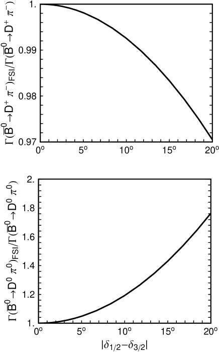
FIG. 1.: The ratio of $\Gamma(\overline{B}^{0}\to D\pi)$ in the presence of final-state interactions (FSI) to that without FSI versus the isospin phase-shift difference. The calculation is done in the NRSX model [12].

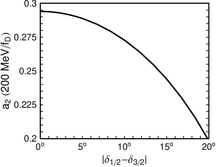
FIG. 2.: The upper bound of the effective coefficient $a_{2}$ multiplied by $(200\,{\rm MeV}/f_{D})$ derived from the current limit on $\overline{B}^{0}\to D^{0}\pi^{0}$ using the NRSX model [12] versus the isospin phase-shift difference.