Phase diagram of 3D $SU(3)$ gauge-adjoint Higgs system and C- violation in hot QCD

Abstract

Thermally reduced QCD leads to three dimensional $SU(3)$ gaugefields coupled to an adjoint scalar field $A_{0}$. We compute the effective potential in the one-loop approximation and evaluate the VEV’s of $TrA_{0}^{2}$ and $TrA_{0}^{3}$. In the Higgs phase not only the former, but also the latter has a VEV. This happens where the $SU(3)$ gauge symmetry is broken minimally with U(2) still unbroken. The VEV of the cubic invariant breaks charge conjugation and CP. It is plausible that in the Higgs phase one has a transition for large enough Higgs selfcoupling to a region where $TrA_{0}^{3}$ has no VEV and where the gaugesymmetry is broken maximally to $U(1)\times U(1)$. For a number of colours larger than 3 an even richer phase structure is possible.

I Introduction

To obtain reliable information about the quark-gluon plasma well above the critical temperature thermally reduced QCD is extremely efficient.

Since its inception[2] it has been pioneered in recent years [7] for a precise evaluation of the Debye mass for $SU(2)$ and $SU(3)$ gauge groups with or without quarks.

In this note we want to point out some properties of the phasediagram of $SU(3)$. These properties have to do with the Higgs phase of the three dimensional gauge-adjoint scalar theory. They are qualitatively different from its $SU(2)$ counterpart.

The main point of this paper is how and what breaking patterns of the various symmetries in the Lagrangian do emerge. R-symmetry breaking ($A_{0}\to-A_{0}$) and gauge symmetry breaking are narrowly related, and we surmise where they are realized in the phase diagram. The Higgs phase in our reduced action is induced by quantum effects. These effects are calculable for a certain range of values of the parameters in the Lagrangian by a loop expansion [9]. This calculation results in a critical line in the phase diagram. Below this line the Higgs phase realizes, with the VEV of $TrA_{0}^{2}$ non-zero. But in $SU(3)$ the VEV of $TrA_{0}^{3}$ is not necessarily zero, and, as we will see, it acquires a VEV in the loop expansion. At the same time the gauge symmetry is minimally broken, leaving a $U(2)$ group unbroken. This phase is obviously absent in $SU(2)$. However a phase where simultaneously R-parity is restored and the gauge symmetry is maximally broken to $U(1)\times U(1)$ is possible and we surmise it is realized in between the symmetric phase and the broken R-parity phase discussed above. This would be a phase in which Abelian monopoles screen the two photons just as in the $SU(2)$ case [4]. Some aspects of the R-parity breaking have been briefly mentioned at LAT98 [13], and in ref. [1].

II Reduced QCD Lagrangian

The Lagrangian of reduced QCD reads:

$$S=\int d\mathchoice{{\hbox{\boldmath$\displaystyle x$}}}{{\hbox{\boldmath$\textstyle x$}}}{{\hbox{\boldmath$\scriptstyle x$}}}{{\hbox{\boldmath$\scriptscriptstyle x$}}} \{ {1\over 2}\sum_{i,j}TrF_{ij}^{2}+\sum_{i}Tr(D_{i}A_{0})^{2}+m^{2}TrA_{0}^{2}$$ (1)

$$+ \lambda_{1}(TrA_{0}^{2})^{2}+\lambda_{2}TrA_{0}^{4}+\delta S\}$$ (2)

If the number of colours is 2 or 3, the quartic terms coalesce to one term, which we will write as $\lambda(Tr{A_{0}}^{2})^{2}$, with $\lambda=\lambda_{1}+\lambda_{2}/2$.

The term $\delta S$ stands for all those interactions consistent with gauge, rotational and R-symmetry (i.e. $A_{0}\to-A_{0}$). These are symmetries respected by the reduction.

We will study the reduced action limited to the superrenormalizable terms in eq. 2, and mostly for $N=3$. The reduced action has a particular raison d’être: its form is given by integrating out the heavy degrees of freedom of QCD at high temperature $T$, with coupling $g$ and number of flavours $N_{f}$. In terms of these parameters we have at one loop accuracy [9]:

$$g_{3}^{2}=g^{2}T$$ (3)

$$m^{2}={1\over 3}\left(N+{N_{f}\over 2}\right)g^{2}T^{2}$$ (4)

$$\lambda_{1}={g^{4}T\over{4\pi^{2}}}$$ (5)

$$\lambda_{2}=(N-N_{f}){g^{4}T\over{12\pi^{2}}}$$ (6)

The gauge coupling $g_{3}^{2}$ has dimension of mass, so the phase diagram is specified by three dimensionless parameters [9] $x_{1}=\lambda_{1}/g_{3}^{2}$ ($x_{2}=\lambda_{2}/g_{3}^{2}$) and $y=m^{2}/g_{3}^{4}$. For N=2,3 there are only two such variables, and we define $x=\lambda/g_{3}^{2}$. The 4D theory lies on the line determined parametrically by the 4D coupling g in eq. 6, i.e. for $N\geq 4$ and to order $O(x_{i})$:

$$x_{2}={1\over 3}(N-N_{f})x_{1}$$ (7)

$$yx_{1}={1\over{12\pi^{2}}}(N+{N_{f}\over 2})$$ (8)

whereas for $N=2,3$:

$$yx={1\over{72\pi^{2}}}(N+{N_{f}\over 2})(6+N-N_{f})+O(x)$$ (9)

It is obvious that $x\sim g^{2}$and $xy\sim\mathrm{constant}$ at very high temperature. Hence the choice of axes in the phase diagram, fig. 3.

In the reduction process, there is a remarkable cancellation, including two loop order, for the coefficients of all renormalizable and nonrenormalizable terms containing only $A_{0}$ [10].

III The effective action

Understanding the phase diagram of the 3D theory necessitates the knowledge of the effective action. We define it for SU(3) with its quadratic and cubic invariants as:

$$\exp{-VS_{eff}(C,E)}=\int DA \delta \left(g_{3}^{2}C-\overline{TrA_{0}^{2}}\right)$$ (10)

$$\delta \left(g_{3}^{3}E-\overline{TrA_{0}^{3}}\right)\exp{-S}$$ (11)

The bar means the average over the volume V. Hence the volume factor in front of the effective action on the l.h.s. in eq. 10. In the large volume limit we can deduce the effective action for $TrA_{0}^{2}$ by minimizing over E, keeping C fixed:

$$min_{\{E\}}S_{eff}(C,E)=V(C)$$ (12)

The effective action for $TrA_{0}^{3}$ follows similarly:

$$min_{\{C\}}S_{eff}(C,E)=W(E)$$ (13)

Note we do not use the 1PI functional as is done frequently [9]. Instead we preferred the the potentials $V(C)$ and $W(E)$, since they are the distributions for the order parameters of relevance to the phase diagram, hence directly measurable (for earlier use of manifestly gauge invariant quantities see [15, 19]). Taking moments of these distributions gives us the average of $TrA_{0}^{p}$, $p=2,3$.

It is very useful to express the effective action $S_{eff}(C,E)$ is in terms of the variables $B_{1},B_{2}$ and $B_{3}$, the diagonal elements of a traceless diagonal $3\times 3$ matrix $B$. This matrix $B$ will be the background field of $A_{0}$(see section 4), and so, apart from the fluctuations discussed in the next section:

$$g_{3}^{2}C=TrB^{2};\hskip 11.38109ptg_{3}^{3}E=TrB^{3}$$ (14)

The matrix $B$ can be expressed in the two diagonal generators of SU(3), normalised at $1/2$, and the azimuthal angle $\theta$ in the $B$ plane:

$$B = \sqrt{2}C^{1/2}\left(\cos\theta\lambda_{8}+\sin\theta\lambda_{3}\right)$$ (15)

The two invariants do fix, up to symmetries (see fig. 1), the azimuthal angle:

$$\cos 3\theta=-\sqrt{6}E/C^{3/2}$$ (16)

In fig. 1 we have plotted the symmetries of the effective action in this plane, due to permutation symmetry of the $B_{i}$ and R-symmetry $B\to-B$. As a consequence the plane is divided in sextants. The circle corresponds to constant $C$. Also shown are the curves of constant $|E|$ in every sextant, and in particular the asymptotes (dashed lines), where $E=0$. These are the directions where the gauge symmetry breaking is maximal, e.g. $\lambda_{3}\sim\mathrm{diag}(1/2,-1/2,0)$. So in the Higgs phase with $TrA_{0}^{2}\neq 0$ the statement that $TrA_{0}^{3}$ has no VEV means the symmetry is broken maximally. The opposite is true too: in the Higgs phase with maximal gauge symmetry breaking the VEV of the cubic invariant is necessarily zero.

FIG. 1.: Permutation and R-symmetry render the potential identical in the six segments between either broken or continuous lines. The former are directions of maximal, the latter of minimal gauge symmetry breaking. The circle is defined by fixing $C$, the cubic invariant $|E|$ fixes the curves with the broken lines as asymptotes.

Is there an analogous statement for the phase where the cubic invariant has a non-zero VEV? That is, does minimal gauge symmetry breaking imply a VEV for $TrA_{0}^{3}$ and vice versa? Look in fig.1 at the positive $\lambda_{8}$ direction. It is clear that there curves of constant $TrA_{0}^{3}\neq 0$ and of constant $TrA_{0}^{2},$ have a common tangent (in the $\lambda_{3}$ direction). So if one invariant has a local minimum there, so has the other. In section V we show explicitely, that both invariants have an absolute minimum in the $\lambda_{8}$ direction. So the answer will shown to be in the affirmative:

In the Higgs phase the cubic invariant is non-zero if and only if the gauge symmetry breaking is minimal, i.e. $U(2)$ is still unbroken.

IV The Higgs phase through the loop expansion

The loop expansion of $S_{eff}$, eq. 2, will be only trustworthy where we find a Higgs phase, hence masses for our propagators. In the symmetric phase Linde’s argument [3] will apply. In addition $x$ should be small. Because the effective potential we use may be less familiar to the reader, we will go into some detail for the case of SU(3). The loop expansion starts from the background field B and admits for small fluctuations around $B$:

$$A_{0} = B+Q_{0}$$ (17)

$$A_{i} = Q_{i}$$ (18)

The gauge invariant constraints have to be taken into account. Most convenient is to introduce two variables $\gamma$ and $\epsilon$ to Fourier analyse the deltafunction constraints in eq. 10. As for the fields, we split them into background and quantum variables: $\gamma=\gamma_{c}+\gamma_{qu}$ and likewise for $\epsilon$. One does do a saddle point approximation around $B$, $\gamma_{c}$ and $\epsilon_{c}$ in the path integral in eq. 10. The linear terms in $\gamma_{qu}$ and $\epsilon_{qu}$ give eq. 14. Linear terms in $\overline{TrBQ_{0}}$ and $\overline{TrB^{2}Q_{0}}$ give respectively equations of motion ($V$ is the volume):

$$-2i\gamma_{c}+V\left(2m^{2}+4\lambda TrB^{2}\right)=0$$ (19)

$$\epsilon_{c}=0$$ (20)

The quadratic part in the expansion of $Q_{0}$ contains a term from the constraint :

$$-i\gamma_{c}\overline{TrQ_{0}^{2}}+3i\epsilon_{c}\overline{TrBQ_{0}^{2}}$$ (21)

apart from the quadratic contribution from the reduced action, eq. 2.

Substituting from the equations of motion (20) into the quadratic part eliminates all terms proportional to $TrQ_{0}^{2}$ and $TrBQ_{0}^{2}$. The saddle point of this observable ignores the presence of the Higgs potential, except that only massterms proportional to $\lambda(TrBQ_{0})^{2}$ stay. So all Higgs masses are zero, except for the diagonal component $TrBQ_{0}$  . The only way they still can get masses is through the gauge fixing. This is essential for the gauge independence of $S_{eff}$, as we shall see now.

By choosing $R_{\xi}$ gauge we eliminate mixed terms between $Q_{0}$ and $\textstyle Q$. The $\xi$ dependence enters only in the masses of the off-diagonal ghosts, longitudinal vectorbosons and Higgs. For a given off-diagonal component (ij), $1\leq i\leq j\leq N$, they all equal $\xi g_{3}^{2}(B_{i}-B_{j})^{2}$. Thus integration over these modes gives cancellation of the gauge dependent masses. The diagonal Higgs do not get a mass from $R_{\xi}$ gauge and the result to one loop order reads:

$$S_{eff}(C,E ) /g_{3}^{6}=yC+xC^{2}$$ (22)

$$- {1\over{3\pi}}\{{1\over{g_{3}^{3}}}\sum_{1\leq i\leq j\leq N}|B_{i}-B_{j}|^{3}+2(xC^{2})^{3/2}\}$$ (23)

The first line is the tree result, the second line the one loop result. The transverse gluons contribute the first, the diagonal Higgs component $TrBQ_{0}$ the second term.

This is valid for number of colours $N=2,3$. Going beyond $N=3$ adds a new invariant $\sim TrA_{0}^{4}$ to the reduced action, eq. 2. It also increases the number of constraints in eq. 10. Remarkably, the new coupling does not show up in the one-loop result as the reader can easily work out from the ensuing saddle point equations. Hence the above result for $S_{eff}$, supplemented with the extra tree term $\lambda_{2}TrB^{4}$ (that is, the quartic invariant) is valid for any N. What is different is the relation of the cubic term, contributed by the transverse gluons, to the quadratic, cubic, quartic etc. invariants, to which we turn now, for the case $N=2$ and $N=3$.

For N=2, ${|B_{1}-B_{2}|}^{3}=2\sqrt{2}C^{3/2}$. For N=3 we found it convenient to work with the azimuthal angle $\theta$ in fig. 1. The potential for SU(3) becomes then::

$$S_{eff}(C,E)/g_{3}^{6}=yC+xC^{2}-{2\sqrt{2}\over{3\pi}}C^{3/2}a(\theta)$$ (24)

$$a(\theta) = |\sin\theta|^{3}+|\sin(\theta+{2\pi\over 3})|^{3}+|\sin(\theta+{4\pi\over 3})|^{3}$$ (25)

$$+ {1\over{\sqrt{2}}}x^{3/2}$$ (26)

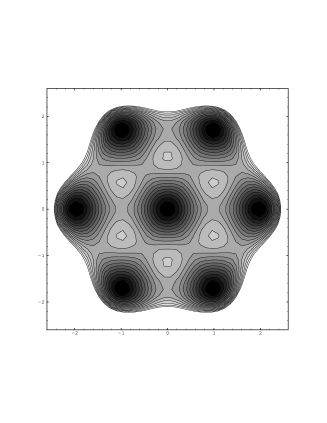
FIG. 2.: The SU(3) potential, eq.(8), on the critical line as explained in the text, at x=0.1. Horizontal and vertical axis as in fig. 1. Dark areas show low, light areas high values.

In fig. 2 we show a contour plot of the potential for N=3 on the curve

$$xy_{c}={3\over{8\pi^{2}}}+{\mathcal{O}}(x)$$ (27)

This is the critical line in the (x,xy) plane of degenerate minima along the $\lambda_{8}$ direction (or its five equivalents). The critical line to this order is identical to the 4D physics line for N=3 in eq. 9. Two loop order (or higher) may distinguish them.

To obtain the potentials (6) and (7) from our explicit result eq. (15) we have a simple analytic proof of where the minima are, but the reader can see by inspection that both the effective potentials for the quadratic and for the cubic invariants are determined by the minimum along the $\lambda_{8}$ direction, using eq. 10 and the curves of constant C and constant E in fig.1. That is, we minimize the effective potential  (10) with respect to $\theta$ and the minima occur at $\theta=0$, mod $2\pi/6$. As a consequence:

$$V(C) = S_{eff}(C,\theta=0)$$ (28)

$$W(E) = S_{eff}(C(E),\theta=0)=V(C(E))$$ (29)

In the last equation we used that this direction, $\theta=0$, relates the VEV’s by:

$$|TrA_{0}^{3}|={1\over\sqrt{6}}(TrA_{0}^{2})^{3/2}$$ (30)

as follows from eq. 16. Hence where the loop expansion is valid the phase with minimal gauge symmetry breaking and R-symmetry breaking realizes.

From the explicit form of the potential for the quadratic VEV, eq. 29 we find the critical line Note that on this line the location of the second minimum is at $C=O(x^{-2})$, and a simple scaling argument shows, that all terms in the effective action (tree and one loop), eq. 29, are of the same order $x^{-3}$. Two loop contributions will be down by a factor x.

It is helpful to observe that the unbroken U(2) symmetry leaves us with two off-diagonal zero mass transverse gauge bosons. This is why in this direction there is a valley. Up to two loops they give no problems. They may get a screening mass from the U(2) monopoles in this phase, much like the Abelian monopoles screen in the SU(2) case the remaining photon [4]. So then the stability of this phase would not only be a matter of small fluctuations around a high VEV (of order $x^{-1}$). There may be an instability, when x is so large, that the valley is no longer a minimum, and a phase transition to a second Higgs phase will occur.

FIG. 3.: Sketch of the SU(3) phase diagram, with unbroken gaugegroups indicated. R-symmetry is only broken in the left lower phase

V A second Higgs phase?

Having established the presence of a phase with minimal symmetry breaking for small x, we have to look for approximation methods at large x. One possibility is mean field with a loop expansion at large values of the lattice coupling and we are analyzing this [10]. Also under study is a lattice Montecarlo study [12].

On the basis of the final remarks in the preceding paragraph one would surmise that transition to come about because the U(2) monopoles become unstable and therefore the contribution of the U(2) transverse vectorbosons grows so large in the $\lambda_{8}$ direction, that the minimum shifts to the $\lambda_{3}$ direction. Along this direction only Abelian monopoles survive, and the cubic VEV is zero (see section III).

As we said earlier, this is the phase where Polyakov’s mechanism is at work [4]. The two photons are screened by the Abelian fields of the ’t Hooft Polyakov monopoles [5]. This phase would in part of the phase diagram (see fig. 3) join smoothly the symmetric phase, like in $SU(2)$.

VI Z(N) invariance and phasestructure for higher N

As noted by the authors of ref. [9] the minus sign in front of the induced cubic term in the effective action, eq. 26, looks formally like an invariance present in 4D when $N_{f}=0$ : $Z(N)$ invariance. This invariance involves a large gauge transformation, in the centergroup of Z(N), $A_{0}\sim{2\pi\over N}T/g$. The reduced theory describes in any of the Z(N) vacua the properties of the plasma at very high T. But it does not pretend to describe what happens in between two Z(N) vacua, like the tunneling which leads to the deconfining transition.

Still, formally it is there in eq. 23, apart from the presence of the term $x^{3/2}(TrB^{2})^{3/2}$, which for x small can be neglected with respect to the term linear in $x$. Since the invariance is a 4D invariance, we can only expect it in the phasediagram of the 3D theory, where $x_{i}$ and $y$ are related to 4D physics, as in eq. 6 and below.

It is well known, to one loop order, that the Z(N) effective potential results from eq. 23 by substituting the 4D parameters from eq. 6 into it [9]:

$$S_{eff}(y,x) = {2\over 3}\pi^{2}T^{3}\sum_{i,j}\tilde{B}_{ij}^{2}(1-|\tilde{B}_{ij}|)^{2}$$ (31)

$$+ O(g^{2})$$ (32)

The dimensionless field $\tilde{B}_{ij}$ stands for the difference of ${g^{2}\over{2\pi}}(B_{i}-B_{j})/g_{3}$. It will be of order one and hence the dimensionless ratio $B_{i}/g_{3}$ is large, of order $g^{-2}\sim x^{-1}$. So the quadratic invariant C will be of order $x^{-2}$, as discussed at the end of section IV.

The resulting surface tension $\alpha$ [18] is for small $x\sim g^{2}$ rewritten in 3D language:

$${\alpha\over{(g_{3}^{2}N)}^{2}}={(N-1)\over{81\pi^{3}}}{1\over{\sqrt{2}}}\left({N+6\over{4N}}\right)^{5/2}{1\over{x^{5/2}}}$$ (33)

This is valid for N=2 and 3. Note it drops when moving to the right on the critical line to larger x, indicating that the transition becomes softer. This is as expected from the SU(2) case [9].

It is amusing to go beyond N=3. The phase diagram is then three dimensional as discussed below eq. 6. Let us take SU(4) as example, with C, E and F as respectively quadratic, cubic and quartic invariants. The effective potential has now a minimum in the direction $\lambda_{15}\sim(1,1,1,-3)$ . The effective potential for C reads:

$$V(C)=yC+x_{1}C^{2}+x_{2}F-{1\over\pi}\left({4\over 3}C\right)^{3/2}$$ (34)

and the potentials W(E) and X(F) for cubic and quartic invariant have the same form as V(C) except for the scaling factors:

$$E=-1/3\sqrt{3}C^{3/2},\hskip 8.53581ptF=7/12C^{2}$$ (35)

In this phase SU(4) breaks to U(3) and the VEV’s of all invariants are non-zero. There is another possible phase, where the unbroken subgroup is U(2) and E=0. For SU(5) there are 3 possible Higgs phases, one with all four invariants a non zero VEV, one with only E=0, and one with only the quintic invariant zero. The critical surface to one loop order is for N arbitrary:

$$y_{c}\left(x_{1}+{(N^{2}-3N+3)\over{N(N-1)}}x_{2}\right)={1\over{36\pi^{2}}}{N^{3}\over{(N-1)}}$$ (36)

This follows immediately from the form of $V(C)$ in the potential valley in the direction of $\lambda_{N^{2}-1}$, and solving for the points $(x_{1},x_{2},y)$, where V(C) develops degenerate minima. It contains the line of 4D physics in eq. 8.

The surface tension now depends on two variables that defines the critical surface and contains as special case the Z(N) surface tension on the physical 4D line.

VII Discussion and comparison with other results

The main finding in this paper, the appearance of a new phase inside the Higgs phase with the help of a new order parameter, was leaning heavily on the use of the distribution function of these order parameters.

Most people practition the 1PI functional, which leads to the same results[9]. as our functional, as we indeed found in this low order case. It is well known that the difference between the two is at most in the constant, VEV independent part. As an example of that the 1PI method through its dependence on the Debye mass reproduces the $O(g^{3})$ term of the free energy in absence of the VEV, whereas our method does not. The reader may be alarmed that in the discussion of the saddle point of our gauge invariant distribution the y parameter, i.e. the Debye mass, did not appear anymore in the propagators of the $A_{0}$, whereas it does in the propagators for the 1PI functional[9]. This feature is just one of the conditions for it to be gauge independent, as we made amply clear in $R_{\xi}$ gauge. The only remnant of the Higgs potential in the propagator of the Higgs is through the quartic coupling, and then only in the neutral component $TrBQ_{0}$.

R parity is up to a colour transposition CP in disguise. The CP transformation in the 4D theory amounts to $A_{0}\to-A_{0}^{T}$ (where T stands for matrix transpose), and $A_{i}\to A_{i}^{T}$. Not only the 4D action, but also its reduced version eq. 2, are invariant under this transformation. So, whenever R-parity is broken, so is CP. In particular, on the 4D physics line, eq. 8 or  9, we have CP spontaneously broken, whenever R parity is broken. The same is true for charge conjugation C.

What remains of this phase structure in the original 4D theory? The $A_{0}$ is the linearized version of the Wilson line. The minimally broken Higgs phase will then map on the Wilson line $P$ in the $\lambda_{8}$ directon and connect to the Z(N) vacua $P=\exp{\pm i{2\pi\over 3}\lambda_{8}}$. This vacuum will obviously not break anymore the gauge symmetry. But C and CP remain broken, because they map the two Z(3) vacua onto one another. In absence of quarks the $Z(3)$ vacua are mapped onto each other by big gauge transformations. But this is not true anymore in the presence of quarks, when the Z(N) vacua become non-degenerate, and can form C or CP violating bubbles. This mechanism and its measurable effects has been discussed in the litterature for strong [20] and electroweak[21] interactions. It is still subject to discussion because of thermodynamic anomalies [22].

This mechanism might become visible in RHIC physics though C-odd observables involving the energy difference of oppositely charged pions. Similar observables have been discussed recently [23] for a mechanism in QCD that creates P-violating bubbles through a quite different approach.

VIII Summary

In summary, we have shown that at least one Higgs phase is realized with spontaneously broken R-symmetry and minimal gauge symmetry breaking. It is fairly plausible that the other phase is located as shown in fig. 3. Montecarlo simulations should test for the additional Higgs phase.

This phase makes it once more clear, that the Higgs phase does not correspond to the physical 4D theory, because the broken R-parity makes it impossible to define a Debye mass! The Debye mass is the lowest state with negative R-parity [6] and such a state is absent in the new phase.

But in the 4D theory, as argued above, this phase could be a reflection of the C violating properties of the Z(N) vacua. No such possibility exists for the minimally broken phase, and the latter is from the point of view of 4D theory an artifact of the reduced theory.

Very interesting is the contrast between the SU(2) and SU(3) monopole case. What about the non-Abelian monopoles in the minimally broken phase in SU(3)? Montecarlo studies as in ref. [14] should reveal their structure. Some analytic progress on classification and dynamics of these monopoles has been made by K. Lee and A. Bais [11]. The rich structure for N larger than 3, briefly mentioned at the end of section IV, may be relevant for the $SU(5)$ transition(see [17]).

REFERENCES

- [1] S. Bronoff, R. Buffa, C. P. Korthals Altes, hep-ph/9809452, Contributing paper to the proceedings of the 5th International Workshop on Thermal Field Theories and their Applications, Regensburg, Germany, August 10-14, 1998.
- [2] T.Applequist,R.D. Pisarski, Phys. Rev D 23 (1981) 2305 P. Ginsparg, Nucl. Phys B 170 (1980), 388; L. Karkainen, P. Lacock, D. E. Miller, B. Petersson and T. Reisz, Nucl. Phys B 418 (1994), 3.
- [3] A. D. Linde, Phys. Lett.B96(1980),289.
- [4] A. M. Polyakov, Nucl. Phys.B120(1977),429.
- [5] G. ’t Hooft, Nucl. Phys.B79(1974), 276.
- [6] P. Arnold, L. Yaffe, Phys. Rev. D52 (1995) 7208.
- [7] K. Kajantie, M. Laine, J. Peisa, A. Rajantie, K. Rummukainen and M. Shaposhnikov, Phys. Rev. Lett. 79 (1997) 3130; M. Laine, O. Philipsen, Nucl.Phys.B523, (1998), 267, F. Karsch, M. Oevers, P. Petrecky, hep-lat/9807035.
- [8] S. Bronoff and al., in preparation.
- [9] K. Kajantie, M. Laine, K. Rummukainen, M. Shaposhnikov, Nucl.Phys.B503, 1997, 357.
- [10] S.Bronoff, thesis, and S.Bronoff, R. Buffa and C. P. Korthals Altes, in preparation. This fact was known to M.Laine, private communication.
- [11] F. A. Bais and B. J. Schroers, Nucl. Phys. B512 (1998); K. Lee, E. J. Weinberg and P. Yi, Phys. Rev. D44(1996), 6351.
- [12] F. Karsch, in preparation, P. Boucaud, in preparation. K. Kajantie, M. Laine, A. Rajantie, K. Rummukainen and M. Tsypin, hep-lat/9811004.
- [13] S. Bronoff, C. P. Korthals Altes, hep-lat/9808042.
- [14] A. Hart, O. Philipsen, J.D. Stack, M. Teper, Phys. Lett. B396 (1997) 217.
- [15] W. Buchmuller, Z. Fodor, A. Hebecker, Phys.Lett.B331,131,1994, hep-ph/9403391
- [16] J. Polonyi, S. Vasquez, Phys. Lett. B240,183,1990.
- [17] A. Rajantie, Nucl. Phys. B501,521,1997.
- [18] T. Bhattacharya, A. Gocksch, C.P. Korthals Altes and R. D. Pisarski, Phys. Rev. Lett.66(1991),998, Nucl. Phys.B383(1992),487.
- [19] C.P. Korthals Altes, Nucl. Phys.B420(1994),637.
- [20] C.P. Korthals Altes, in “Gauge theories, Past and Future” conference proceedings in commemoration of the 60th birthday of M. Veltman; eds R. Akhoury, B. de Wit, P. van Nieuwenhuizen, H. Veltman, (World Scientific series in 20th century physics, 1992). World Scientific, Singapore,1992.
- [21] C.P. Korthals Altes, K. Lee, R. D. Pisarski, Phys.Rev.Lett.73,1754(1994); C.P. Korthals Altes and N.J. Watson, Phys. Rev. Lett. 75(1995) 498.
- [22] V.M. Belyaev, I.I. Kogan,G.W. Semenoff and N. Weiss, Phys. Lett. B227(1992),331. See however S.Bronoff, C. P. Korthals Altes, in the Proceedings of the Conference on Continuus Advances in QCD 1996, pg 185. Ed. M. I. Polikarpov, World Scientific, Singapore.
- [23] D. Kharzeev, R.D. Pisarski amd M. Tytgat, Phys.Rev. Lett.81,512 (1998)