Small-$\boldsymbol{x}$ one-particle-inclusive quantities in the CCFM approach

Abstract:

This article presents the results of a quantitative study of the small-$x$ data at HERA, using the CCFM equation. The first step consists of choosing the version of the CCFM equation to be used, corresponding to selecting a particular subset of next-to-leading-logarithmic corrections — the choice is constrained by requiring a phenomenologically reasonable small-$x$ growth. For the time being, the parts of the splitting functions that are finite at $z=0$ have been left out. We then examine results for $F_{2}^{c}$, $R$, the transverse energy flow, the charged-particle transverse-momentum spectrum and the forward-jet cross section and compare to data. While some of the data is reproduced better than with DGLAP-based calculations, the agreement is not entirely satisfactory, suggesting that the approach developed here is not yet suitable for detailed phenomenology. We discuss why, and suggest directions for future work.

1 Introduction

The HERA accelerator has opened up a radically new region of phase space for Deep Inelastic Scattering (DIS). This is the region where Bjorken-$x$ is very small, while the photon virtuality $Q^{2}$ is still hard but moderate. In this kinematical domain it is no longer clear that DGLAP evolution [1], which resums logarithms of $Q^{2}$, should lead to a good description of the physics. Indeed one expects that the resummation of logarithms of $1/x$ should become equally if not more important. One of the aims of the HERA experiments is to study observables which have different characteristics according to the kind of resummation performed, in order to clarify one’s understanding of the kinematical domain and of the details of the resummation of logarithms of $x$.

For total cross sections (i.e. DIS structure functions), leading logarithms of $1/x$ ($\alpha_{\mbox{\scriptsize s}}^{n}\ln^{n}1/x$) can be resummed using the BFKL equation [2]. This predicts that the total cross section should grow as a power of $1/x$. The rapid rise of the $F_{2}$ structure function at small $x$ [3, 4], when first discovered, was optimistically hailed as being evidence for this. There are however difficulties with such a claim at a quantitative level:

1. With DGLAP-based approaches the data can be quite straightforwardly fitted, using either an input parton distribution which rises at small-$x$, or by starting the evolution from a low scale [5, 6].

2. Leading logarithmic (LL) BFKL evolution leads to much too steep a rise of $F_{2}$ to allow a fit to the data (see e.g. [7]).

3. The recently calculated next-to-leading (NLL) corrections to the BFKL kernel [8, 9] turn out to dominate over the leading contribution for any realistic value of the strong coupling (so perhaps it should come as no surprise that leading-order BFKL cannot fit $F_{2}$), and if taken literally, lead to nonsensical results [10].

4. BFKL evolution is not ordered in transverse momentum, as a result of which diffusion in transverse momentum [11, 12, 13] leads to significant dependence on the infra-red region, where the perturbative series is irretrievably out of control.

Points two and three are closely connected, and in due time, perhaps following an approach similar to that of [14], we will probably learn how to resum large parts of the NLL corrections. One can to some extent avoid the problems of the infrared region by including small-$x$ resummations in the $Q^{2}$-evolution of the $F_{2}$ structure function [15]; the tradeoff is that as in DGLAP, one needs an input parton distribution over the whole range of $x$, possibly leaving a little too much freedom in fitting the data.

A way of observing BFKL phenomena while avoiding sensitivity to poorly known input parton distributions or to the infrared region was suggested some time ago by Mueller and Navelet [16] in their proposal to study more exclusive quantities, in particular the cross section for the production, in hadron-hadron collisions, of two similarly hard jets separated by a large rapidity interval, which should grow as an exponential of that rapidity interval. The advantage of this observable (and of many other similarly exclusive measurements which have since then been proposed), is that by triggering on two large transverse momenta at the extremes of the evolution, one can suppress the probability of diffusion into the infra-red region, leaving a quantity which can, at least in principle, be calculated perturbatively (of course if the rapidity interval between the two transverse momenta becomes too large, then diffusion once again becomes important). A second advantage is that such observables can discriminate between BFKL and DGLAP evolution more effectively than the total cross section at small $x$: DGLAP evolution cannot possibly mimic the expected BFKL behaviour, because generally the two transverse scales are of the same order, and DGLAP only enhances cross sections for interaction between objects with very different transverse scales.

So an efficient way to identify the most important characteristics features of $\ln x$ resummation is to study the final state. It turns out that the multi-parton distribution of an event cannot be reliably obtained from the BFKL equation. The fundamental additional element that must be taken into account (as in almost any calculation of final-state properties [17]) is that of the coherence of QCD radiation [18]. For the particular case of an evolution in which the transverse scale increases along the direction of evolution, the correct formulation was derived in [19] and is known as the CCFM equation — it correctly resums the leading $\ln 1/x$ and $\ln Q$ terms both for inclusive and non-inclusive quantities [20]. Angular ordering should also reduce the dependence on the infra-red region, since large drops in the transverse scale are disfavoured, thus limiting diffusion [21].

In contrast to the BFKL and DGLAP equations, whose parton densities depend on two variables (energy fraction and transverse momentum), the CCFM gluon density depends additionally on a limiting angle. This increases very considerably the mathematical complexity of the equation, and it can only be solved numerically (and even that is highly non-trivial).

In view of this difficulty one is led to ask whether it is really necessary to use the CCFM equation in order to get a valid description of the final state. It has been pointed out by Ryskin [22] that if one formulates the BFKL equation as an evolution in rapidity rather than in $x$, then one automatically has angular ordering. This for example is the approach that has been taken by Orr and Stirling [23] in calculating Mueller-Navelet-like two-jet observables at the Tevatron, and in such a context it may be valid.

However the point of the CCFM equation is not simply that of angular ordering — rather it consists in the combination of the ordering of angles and the ordering of the $x$ variables, in a situation in which transverse momenta increase along the chain, i.e. a DIS-type situation. If one applies the BFKL equation with only rapidity ordering to a DIS situation then one will obtain an answer for the cross section with spurious double transverse logarithms ($\alpha_{\mbox{\scriptsize s}}^{2}\ln 1/x\ln^{2}Q$) at NLL order. This problem is closely connected with that of the choice of scale in the kernel [9, 14] — indeed in the language of [9], the BFKL equation with rapidity ordering corresponds to choosing a symmetric scale $k_{1}k_{2}$ in the LL kernel. What this means in practice is that the cross section at small $x$ and large $Q^{2}$, instead of behaving, as it should do, as

$$\exp\left(2\sqrt{\frac{{\bar{\alpha}}_{\mbox{\scriptsize s}}C_{A}}{\pi}\ln\frac{1}{x}\,\ln Q^{2}}\right)\,,$$

goes as

$$\exp\left(2\sqrt{\frac{{\bar{\alpha}}_{\mbox{\scriptsize s}}C_{A}}{\pi}\ln\frac{Q}{x}\,\ln Q^{2}}\right)\,.$$

It turns out though, that even the BFKL equation with ordering in $x$ (which does not suffer from the above problem) manages to reproduce correctly certain properties of the CCFM final state: in a fixed-order calculation by Forshaw and Sabio Vera [24], subsequently extended to all orders by Webber [25] it was demonstrated that in the double-logarithmic approximation all one-particle inclusive quantities have the same leading-logarithmic terms in both approaches. Nevertheless one should be wary of such a result, since there is the distinct possibility of one-particle-inclusive quantities having a collinear divergence at subleading order in BFKL [26], and secondly, BFKL may not correctly reproduce correlations between emissions [27, 26].

So it is likely that the CCFM equation is the best approach currently available for studying the final state. At the same time it should be noted that the CCFM equation is not entirely free of problems. Its approximation of ordering simultaneously in angles and $x$ is valid when the transverse scales increase along the direction of evolution. When the transverse scales decrease, the relevant approximation is that of ordering simultaneously in angles and $\bar{x}$. One of the characteristics of small-$x$ evolution is that even if, predominantly, the transverse scale increases (as in DIS), there are evolution steps in which it drops (diffusion) — and the CCFM equation is subject to large subleading corrections in those steps (again this is related to the issue of the choice of scales). One might be tempted to argue that in DIS the problem arises only occasionally and so will not matter excessively — but several final-state “BFKL-signals” at HERA tend to favour evolution paths in which the evolution has no dominant direction in transverse momentum.

Other problems that arise are connected with two further subleading elements of the CCFM equation: the treatment of factors of $(1-z)$ in the kinematical variables of the virtual corrections is not defined at LL order, and as we will see, a modification of their treatment can lead to very large subleading corrections. Secondly the part of the splitting function which is finite as $z\to 0$,

$$-2+z(1-z)+\frac{1}{1-z}$$

can also give important subleading corrections. There are several possible ways of including it in the evolution, and they may well give significantly different subleading corrections. Because of the enhancement at $z=1$, these contributions are quite difficult to study numerically. It should be noted that they (in particular the $1/(1-z)$ part) are vital for a correct description of infra-red sensitive final-state properties.

In this uncertain theoretical context, one thing is clear however: experimentally, DGLAP-based approaches (whether Monte-Carlo event generators or NLO calculations) are incapable of describing many of the small-$x$ final-state observables that are supposed to be sensitive to BFKL phenomena [28, 29, 30, 31]. So there is an urgent need for some BFKL-based phenomenology, and in particular a Monte Carlo event generator based on a leading $\ln x$ resummation. This article is in some sense intended as a study of the extent to which one can carry out quantitative phenomenology using the CCFM equation as it stands currently.

At this point, it is worthwhile specifying some realistic aims. Quite a significant issue is whether one should worry about matching the NLL corrections calculated for the BFKL equation [8, 9]. If they were small, the answer would obviously be “yes.” But since they are so large, all that should matter in practice is the resummed corrections. Some idea of what a (partially) resummed result might look like for the BFKL equation is given in [14]. Beyond this we are limited to being guided by the experimental data. In particular, we aim to reproduce the total cross section as a function of $x$ and $Q^{2}$. This will force us to deal with problems associated with the treatment of the infrared region.

Bearing in mind these requirements, our approach is as follows: we choose a CCFM evolution equation which phenomenologically seems to have a reasonable exponent (i.e. growth at small $x$). By “phenomenologically reasonable,” we mean that for the relevant values of $\alpha_{\mbox{\scriptsize s}}$ it should be roughly consistent with the growth of $F_{2}$, and with expectations from a resummation of NLL terms of the BFKL kernel (as for example, at an approximate level, in [14]). The methods used to determine the exponent follow on from those of [21]. Because of the lack of a well-defined way of including the $z\to 0$ finite part of the splitting function, and because of the considerable difficulty in implementing each new way that one might invent, we simply leave it aside, for possible inclusion at a later stage.

We then develop a suite of programs allowing us to study structure functions and one-particle inclusive quantities, and constrain the treatment of the infra-red region by fitting to the $F_{2}$ structure function data. At this point we should be in a position to give relatively parameter-free predictions for other structure functions ($F_{2}^{c}$, $F_{L}$) and various (almost) one-particle-inclusive final-state quantities: the transverse energy flow, charged particle spectra and the forward-jet cross section.

Before entering into the details it should be noted that there are already in existence a number of programs based on the CCFM equation, for studying small-$x$ DIS scattering.

In [32] there have been studies of the $F_{2}$, $F_{2}^{c}$ and $F_{L}$ structure functions using the form of the CCFM equation without the $z\to 0$ finite part of the splitting function, and with all other $1-z$ factors replaced by $1$ (both in the real and virtual corrections).

The program SMALLX [33] is a direct Monte Carlo implementation of the CCFM equation. It includes the $z\to 0$ finite part of the splitting function (unlike the results presented here), and additionally, the exact kinematic constraints. The main problem with this program is that it is a forward-evolution event generator, with weights that have extremely large fluctuations. This renders it somewhat unwieldy to use. Additionally, though it contains all the physics, there is no way of modifying the exact implementation of the subleading corrections — such modifications turn out to have large effects. The SMALLX program has recently been used and studied in [34], for the case of the production of charm quarks — unfortunately the precision of the data for charm quark production is rather poor (the tagging of open charm is not a simple task), and there is little final-state data available.

Another major numerical study is based on the Linked Dipole Chain (LDC) model [35], which has been implemented as a Monte Carlo event generator [36]. Formally it is based on the CCFM equation with some simplifications and modifications. Perhaps the most important modification is that the evolution has been made symmetric (i.e. it is equally valid whether the transverse scale increases or decreases along the direction of evolution). A lack of symmetry is one of the main defects of the CCFM equation. On the other hand, the LDC model has the problem that it rearranges the real and virtual terms of the evolution in a manner which alters the LL small-$x$ evolution. Whether this is a serious problem is to some extent a question of opinion — after all, given that the known NLL corrections are so large, what really matters phenomenologically is the resummed evolution, not its perturbative expansion. The LDC approach gives satisfactory results for the structure function data and some final state properties such as the transverse energy flow. However it has problems with the charged-particle transverse momentum spectrum and with the forward-jet cross section. As will be seen, our approach has rather similar problems — a discussion of this will be given in the conclusions.

The structure of this paper is as follows: in section 2 we review the structure of the CCFM equation, discuss approximations that are commonly made when solving it, together with the treatment of subleading corrections in the non-Sudakov form factor. In section 3 we examine the asymptotic exponents of various versions of the CCFM equation. In section 4 we consider the evolution parameters and corresponding fits to the $F_{2}$ structure function, as well as the consequences of these different fits for $F_{2}^{c}$ and $R$. In section 5 we then discuss the determination of one-particle-inclusive final-state quantities, and present results. The whole approach, and directions for future work are finally examined in the light of these results in section 6.

In an appendix we give details of a novel analytic approach for implementing the off-shell boson-gluon fusion [37, 38, 39], which is convolved with the unintegrated gluon structure function to give physical cross sections. Traditional approaches generally require a two-dimensional numerical integration over the quark-antiquark phase-space (or alternatively a treatment in terms of the Mellin transform) — the solution presented here carries out these integrations analytically, even in the presence of massive quarks, greatly simplifying the determination of physical cross sections from the unintegrated gluon structure function.

2 Angular ordering

2.1 Kinematics

In what follows, we discuss the unintegrated gluon density of a proton (taken to be massless) with energy $E_{p}$. This gluon density, ${\cal{A}}(x,k,p)$, depends on: $x$, the fraction of the proton’s plus-momentum component that is carried by the gluon; $k$ the gluon’s transverse momentum; and $p$, which defines the maximum-allowed angle of all emissions prior to this gluon, through the relation $p=2xE_{p}\tan\theta_{\max}/2$, where $E_{p}$ is the proton energy. The recipe for choosing $p$ in DIS will be discussed later.

The angular ordering condition on the last emitted gluon (with transverse momentum $q_{t}$ and plus-momentum fraction $x(1/z-1)$) can be written as

$$p>\frac{zq_{t}}{1-z}\,=\,zq\,,$$

where for convenience we have introduced the variable $q=q_{t}/(1-z)$. We shall also use the rapidity $\eta$ of an emitted particle:

$$\eta=\frac{1}{2}\ln\frac{q_{-}}{q_{+}}=\ln\frac{zq}{2xE_{p}}\,,$$ (1)

where, $q_{\pm}=q_{0}\pm q_{3}$ and the proton has a positive 3-component. For the purpose of the kinematics, emitted gluons will always be taken to be massless.

Figure 1: Kinematics of the branching process: $k_{in}$ is momentum coming from proton; $k_{n}$ is momentum entering into the photon-gluon fusion quark-box.

Considering a general branching (see figure 1), in which a space-like gluon $k_{n}$ has transverse momentum ${\vec{k}}_{n}$ and momentum fraction $x_{n}$, and an emitted gluon $q_{n}$ has transverse momentum ${\vec{q}}_{t,n}$, then the general ordering is $q_{n+1}>z_{n}q_{n}$ (with $z_{n}=x_{n}/x_{n-1}$ and ${\vec{q}}_{n}={\vec{q}}_{t,n}/(1-z_{n})$), with ${\vec{k}}_{n}={\vec{k}}_{n-1}-(1-z_{n}){\vec{q}}_{n}$. Additionally all the $q_{t,n}$ satisfy $q_{t,n}>\mu$ where $\mu$ is our collinear cutoff.

The $1-z_{n}$ factor is necessary for the exact reconstruction of the transverse momenta (alternatively, one can interpret it as being necessary for exact angular ordering). It gives a next-to-leading contribution to the structure function evolution (as does angular ordering itself).

2.2 The CCFM equation

The equation satisfied by the unintegrated gluon structure function, ${\cal{A}}(x,k,p)$ is

$${\cal{A}}(x,k,p)={\cal{A}}^{(0)}(x,k,p)+\\ \int_{x}^{1}\frac{dz}{z}\int\frac{d^{2}q}{\pi q^{2}}\,{\bar{\alpha}}_{\mbox{\scriptsize s}}\left(q_{t}\right)\;{\cal{A}}(x/z,|{\vec{k}}+{\vec{q}}_{t}\,|,q)\;\Delta(z,k,q)\Theta(p-zq)\,,$$ (2)

where ${\bar{\alpha}}_{\mbox{\scriptsize s}}=\alpha_{\mbox{\scriptsize s}}C_{A}/\pi$ and ${\vec{q}}_{t}=(1-z){\vec{q}}$. The non-Sudakov form factor (virtual correction) is

$$\ln\Delta(x,k,q)=-\int_{x}^{1}\frac{dz}{z}\int\frac{d^{2}q^{\prime}}{\pi{q^{\prime}}^{2}}\,{\bar{\alpha}}_{\mbox{\scriptsize s}}({q_{t}}^{\prime})\,\Theta(k-Tq^{\prime})\,\Theta(q^{\prime}-zq)\,.$$ (3)

It is usual to set $T=1$, however at leading-logarithmic order it is equally valid to choose $T=1-z$. A motivation for choosing the latter form is that in the real emission term, one has a dependence on ${\vec{k}}+(1-z){\vec{q}}={\vec{k}}+{\vec{q}}_{t}$; one can argue that in analogy, since $q^{\prime}$ is a rescaled transverse momentum, $q^{\prime}=q^{\prime}_{t}/(1-z)$, it is $\Theta(k-q_{t}^{\prime})$ and not the more usual $\Theta(k-q^{\prime})$ which should appear in the form factor. More formally the choice $T=1-z$, at first sight, looks like it ought to cancel the contribution from all emissions with $q_{t}<k$.

The two choices will be discussed in more detail in section 3.

2.3 The initial condition

To ensure a sensible initial condition (one which leads to a collinear safe result after evolution), ${\cal{A}}^{(0)}$ should correspond to the distribution for a Reggeised gluon. Relating to a normal, “non-Reggeised,” initial condition, ${\cal{A}}^{(\mathrm{init})}$, we have

$${\cal{A}}^{(0)}(x,k,p)=\int_{z}^{1}\frac{dz}{z}\,\frac{d{\cal{A}}^{(\mathrm{init})}(z,k)}{d\ln 1/z}\,\Delta(x/z,k,\mu)\,.$$ (4)

The form that we take for ${\cal{A}}^{(\mathrm{init})}(x,k)$ is

$${\cal{A}}^{(\mathrm{init})}(x,k)={\cal{N}}\frac{n+1}{\pi k_{0}^{2}}\,(1-x)^{n}\,\mathrm{e}^{-k^{2}/k_{0}^{2}}\,,$$ (5)

with ${\cal{N}}$, $n$ and $k_{0}$ parameters to be discussed below. Note that ${\cal{A}}^{(0)}(x,k,p)$ does not depend on $p$. The normalisation is such that

$$xg(x,Q^{2})=\int d^{2}k\,{\cal{A}}(x,k,Q)\,,$$

where $g(x,Q^{2})$ is the gluon density in the proton; ${\cal{N}}$ is the result of the energy sum rule for the initial condition:

$${\cal{N}}=\int d^{2}kdx{\cal{A}}^{(\mathrm{init})}(x,k)\,.$$ (6)

2.4 The running coupling

We use the one-loop running coupling, taking $q_{t}$ as its scale (in accord with the results obtained from the NLL calculation [9]). Since $q_{t}$ kinematically can go down to small values, it is necessary to introduce a prescription for the running of $\alpha_{\mbox{\scriptsize s}}$ at low scales: we modify $\alpha_{\mbox{\scriptsize s}}$ so that it reaches a plateau in the infra-red region:

$$\alpha_{\mbox{\scriptsize s}}(q_{t})=\frac{1}{b_{0}\ln(q_{t}^{2}+\Lambda_{0}^{2})/\Lambda^{2}}\,,$$ (7)

with

$$b_{0}=\frac{11C_{A}-2n_{f}}{12\pi}\,,$$

and $\Lambda_{0}$ chosen so as to ensure that $\alpha_{\mbox{\scriptsize s}}(0)=\alpha_{\mbox{\scriptsize s}}^{(0)}$, with $\alpha_{\mbox{\scriptsize s}}^{(0)}$ a parameter; finally, we take $n_{f}=4$ and $\Lambda=0.135$ GeV.

2.5 Parameters

To summarise, the parameters that must be chosen are the following: $\alpha_{\mbox{\scriptsize s}}^{(0)}$, the value of $\alpha_{\mbox{\scriptsize s}}$ at which it freezes, a cutoff on emitted transverse momenta $q_{t}>\mu$ (and $q_{t}^{\prime}>\mu$ in the virtual corrections), and the parameters which affect the properties of the initial condition, ${\cal{N}}$, $n$ and $k_{0}$. They will be constrained by requiring a good fit to the $F_{2}$ structure function, as discussed in section 4. One consistency check of our approach will be that it is possible to find a set of fit parameters that is in accord with one’s physical expectations. For example the normalisation should be such that the energy sum rule should integrate to ${\cal{N}}\simeq 0.5$; $k_{0}$ is expected to be of the order of $1$ GeV; $\alpha_{\mbox{\scriptsize s}}^{(0)}$ should be of the order of $0.5$; and $n\simeq 4$.

Parameters that are only weakly constrained by $F_{2}$ should then be varied to probe their effect on final state quantities.

3 Asymptotic exponents

Figure 2: The asymptotic exponent of the BFKL equation and various forms of the CCFM equation, as a function of $\alpha_{\mbox{\scriptsize s}}$. The “BFKL $+$ NLL” curve is the resummed result (scheme 3) of [14].

Before engaging in a fit of the $F_{2}$ structure function, it is helpful to study, as a function of fixed $\alpha_{\mbox{\scriptsize s}}$, the “asymptotic exponents,” $\omega$, of the various forms of the CCFM equation, since this will indicate which one is most likely to be in accord with the phenomenology (though it should be borne in mind that $\omega(\alpha_{\mbox{\scriptsize s}})$ is not physically observable). The technique adopted is based on that developed in [21]:

$$\omega=\frac{d}{d\ln x}\ln A(x,k,p)\,,$$ (8)

with $x$ sufficiently small that the result is independent of $x$, $k$, and $p$. In the BFKL case, $\omega={\bar{\alpha}}_{\mbox{\scriptsize s}}4\ln 2$.

Figure 2 shows the asymptotic exponents of several versions of the CCFM equation, compared to the BFKL equation, as a function of $\alpha_{\mbox{\scriptsize s}}$. The three versions of the CCFM equation are as follows: the case “$1-z\to 1$” corresponds to (2) and (3) with all $1-z$ factors replaced by $1$ (also in the relation between $q$ and $q_{t}$). This is an approximation quite commonly used (studied for example in some detail in [21]) because it greatly simplifies the numerical solution. However it leads to a slight violation of the angular ordering (or to an incorrect reconstruction of the transverse momenta, depending on whether one interprets $q$ as a real, or a rescaled transverse momentum). The other two versions of the CCFM equation implement the correct treatment of angular-ordering (or transverse-momentum reconstruction), but differ in their treatments of the form factor. The $T=1$ case corresponds to the version of the CCFM equation more commonly quoted.

One sees immediately that the $1-z\to 1$ and $T=1$ cases have exponents which are rather similar to that of the leading-logarithmic BFKL equation. In particular one sees that for the values of $\alpha_{\mbox{\scriptsize s}}$ which are typical in HERA physics, namely $0.2$–$0.3$, the exponents are far above anything observed experimentally. In a non-asymptotic situation (i.e. $x$ not infinitely small) these exponents can be reduced by the introduction of a large collinear cutoff, but, it turns out, not sufficiently to allow a fit to the data.

So the version of the CCFM equation that we will concentrate on in the remainder of this article will be that with $T=1-z$. One can calculate numerically its next-to-leading correction to the exponent, which turns out to be extremely large: $\omega=4\ln 2{\bar{\alpha}}_{\mbox{\scriptsize s}}-(75\pm 4){\bar{\alpha}}_{\mbox{\scriptsize s}}^{2}+{\cal O}\left({\alpha_{\mbox{\scriptsize s}}^{3}}\right)$. This is to be compared with $\omega=4\ln 2{\bar{\alpha}}_{\mbox{\scriptsize s}}-17.91{\bar{\alpha}}_{\mbox{\scriptsize s}}^{2}$ in the case of the full NLL BFKL corrections ($n_{f}=0$) [8, 9]. One is immediately induced to ask why setting $T=1-z$ produes such a large correction. Qualitatively, it leads to large negative virtual corrections from $q_{t}^{\prime}\lesssim k$ for $z$ close to $1$. However the corresponding real-emission contribution, $q_{t}\lesssim k$ for $z$ close to $1$, turns out to be dynamically suppressed because it corresponds to a large emission angle, which reduces the phase space available for subsequent emissions. Consequently the asymptotic exponent receives a large negative correction.

Another question is whether it matters that the NLL correction is so much larger than the true one. One can argue not, since the pure NLL correction turns out to be visible only for extremely small values of $\alpha_{\mbox{\scriptsize s}}$, while phenomenologically we are interested in the region $\alpha_{\mbox{\scriptsize s}}\simeq 0.2$, where formally more subleading corrections (e.g. NNLL etc.) are just as important. So what matters should be the resummed asymptotic exponent, and from figure 2 it seems that this quantity is roughly in line with phenomenological expectations. In fact if one carries out a partial resummation of subleading corrections to the exact NLL BFKL exponent (the curve shown in figure 2 corresponds to scheme 3 of[14]), one obtains a result which is not so different from that with the equation being used here.

Having completed the discussion of the asymptotic exponent, it is however vital to remember that much of the HERA data is to be found in regions of $x$ (or energy) which may be quite far from asymptotic.

4 Structure functions

4.1 Convolution with the quark box

To obtain a result for the $F_{2}$ structure function (or any other cross section) it is necessary to perform the convolution of the unintegrated gluon density ${\cal{A}}(x,k,p)$ with the boson-gluon fusion matrix element (which is discussed in the appendix):

$$F_{2}(x,Q^{2})=\sum_{q}e^{2}_{q}\int_{x}^{1}\frac{dz}{z}\int\frac{dk}{k}{\hat{\sigma}}_{F_{2}}(z,k^{2},Q^{2},m^{2}_{q}){\cal{A}}(x/z,k,p)\,.$$ (9)

In a similar way, one can determine $F_{L}$ and $F_{2}^{c}$. The maximum angle is taken, as in the program SMALLX [33], to be defined by the rapidity of the combined $q\bar{q}$ pair

$$p^{2}=\frac{Q^{2}}{z(1-z)}\,.$$

Modifying this limit would alter our results at next-to-leading order. The light quarks are taken to be massless, while for the heavy quarks we use $m_{c}=1.5$ GeV and $m_{b}=5.0$ GeV. The convolution is performed in a frame in which the proton and photon are collinear and along the $z$-axis (this differs from the laboratory frame by a rotation and a boost). Correspondingly, transverse momenta for final-state quantities are also determined in such a frame.

As discussed in the appendix, $\hat{\sigma}$ is determined entirely analytically. This is in contrast to other approaches, which generally leave $\hat{\sigma}$ in the form of a double integral which must be evaluated numerically [37, 38, 39, 40, 41]. The reduction in the number of numerical integrations simplifies considerably the implementation of the convolution. The only disadvantage is that the analytic integration must be performed with fixed $\alpha_{\mbox{\scriptsize s}}$ — so the value that we use is given by the logarithmic mean of $\alpha_{\mbox{\scriptsize s}}$ between scales $\sqrt{k^{2}+m^{2}_{q}}$ and $\sqrt{Q^{2}+m^{2}_{q}}$:

$$\langle\alpha_{\mbox{\scriptsize s}}\rangle=2\left(\ln\frac{Q^{2}+m^{2}_{q}}{k^{2}+m^{2}_{q}}\right)^{-1}\int_{\sqrt{k^{2}+m^{2}_{q}}}^{\sqrt{Q^{2}+m^{2}_{q}}}\frac{dq}{q}\,\alpha_{\mbox{\scriptsize s}}(q)\,.$$ (10)

In the limits $k\ll Q$ and $k\gg Q$ this gives the correct overall dependence on the running coupling (possibly incorrect with respect to details of the treatment of the quark mass).

4.2 Structure function results

Figure 3: Fits to the $F_{2}$ structure function, compared with H1 [3] and ZEUS [4] 1994 data points.

The fit for the structure function is performed in the kinematic range $x<10^{-2}$ and $8<Q^{2}<140$ GeV². The parameters to which the fit is most sensitive are $\mu$, the collinear cutoff, and $\alpha_{0}$, the value at which $\alpha_{\mbox{\scriptsize s}}$ freezes. We find that $0.01\lesssim\mu\lesssim 0.1$ GeV, and $\alpha_{0}\sim 0.5$ lead to reasonable fits of the H1 and ZEUS 1994 structure function data [3, 4]; as one would expect, there is relatively little dependence on the value of $n$ (the power of $(1-x)$ in the initial condition, see (5)), though it does affect the fitted value of ${\cal{N}}$. It turns out that for the $k$-dependence of the initial condition, $\propto e^{-k^{2}/k_{0}^{2}}$, there is a correlation between the value of $k_{0}$ and the optimal value of $\mu$. Good fits are obtained with a range of $k_{0}$: we will use $k_{0}=1$ GeV, and then examine the effect on other quantities of varying it. Modifying $k_{0}$ by a factor of $2$ (and changing $\mu$ and $\alpha_{0}$ accordingly) affects the normalisation by about $50\%$.

The set of parameters that will be used is as follows:

$\mu$	$0.075$ GeV
$\alpha_{\mbox{\scriptsize s}}^{(0)}$	$0.60$
$k_{0}$	$1.0$ GeV
$n$	$4$
${\cal{N}}$	$0.72$

A comparison with the data is shown in figure 3, and is seen to be in good agreement. The $\chi^{2}$ are $64.4$ for $59$ H1 points [3] and $84.7$ for $80$ ZEUS points [4].

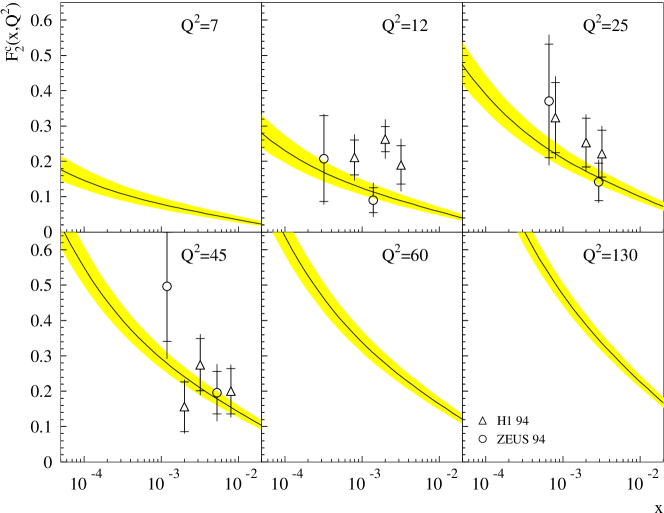
Figure 4: Results for $F^{c}_{2}$ compared with H1 1994 data [42], and ZEUS 1994 data [43].

Using the above fit parameters one can give expectations for the charm structure function and $R$, the ratio of longitudinal to transverse structure functions. The uncertainty on the charm structure function is gauged by varying the charm mass between $1.3$ and $1.7$ GeV. The results are shown in figure 4. There is some indication that our curves are low compared to the data.

Figure 5: $R$

The results for $R$, shown in figure 5, are concentrated around $R\simeq 0.2$ fairly independently of $x$ and $Q^{2}$. This seems to be fairly typical of results from BFKL-based calculations (see for example [44]).

Before moving on to a discussion of final-state quantities, it is perhaps worth commenting on some rather unexpected properties of the $T=1-z$ form of the CCFM equation: as one decreases the cutoff $\mu$, the steepness of the small-$x$ growth decreases. The reason for this unusual behaviour, is that increasing $\mu$ removes from the virtual corrections a region which was already dynamically suppressed in the real emissions (see the discussion in section 3) thus eliminating a negative contribution to the evolution, and increasing the small-$x$ growth. On the other hand, as is more normal, increasing $\alpha_{\mbox{\scriptsize s}}^{(0)}$ increases the small-$x$ growth (though not as substantially as in the pure BFKL case). As a result the best fits tend to favour a diagonal band in the $\alpha_{0}$, $\ln\mu$ space.

This is to be contrasted with the behaviour that one sees with the BFKL equation or with the CCFM equation with $T=1$, where the small-$x$ growth increases as one decreases $\mu$ (there is none of the dynamic non-cancellation between real and virtual parts which is seen with $T=1-z$). We note that if one tries to fit the structure function using BFKL, or CCFM with $T=1$ evolution, then to suppress the small-$x$ growth sufficiently to fit the data, one requires an unphysically large collinear cutoff $\mu\simeq 3$ GeV.

5 One-particle inclusive quantities

A number of final-state properties measured at HERA can be approximated by one-particle-inclusive quantities. The latter are relatively straightforward to calculate with the CCFM equation once one has in place an approach for solving for the evolution of the unintegrated gluon distribution.

Suppose that one is interested in determining the number density of particles entering into a certain region of phase space with a given transverse momentum ${\bar{q}}_{t}$ and rapidity ${\bar{\eta}}$. It is convenient to introduce an intermediate gluon density ${\cal{B}}_{{\bar{q}}_{t}{\bar{\eta}}}(x,k,p)$ which is obtained by considering configurations with any number of emissions, followed by an emission into the region of interest:

$${\cal{B}}_{{\bar{q}}_{t}{\bar{\eta}}}(x,k,p)=\int_{x}^{1}\frac{dz}{z}\int\frac{d^{2}q}{\pi q^{2}}\,{\bar{\alpha}}_{\mbox{\scriptsize s}}\left(q_{t}\right)\;{\cal{A}}(x/z,|{\vec{k}}+{\vec{q}}_{t}\,|,q)\\ \times\Delta(z,k,q)\;\Theta(p-zq)\;\delta({\bar{q}}_{t}-q_{t})\;\delta\left({\bar{\eta}}-\ln\frac{zq}{2xE_{p}}\right)\,.$$ (11)

To obtain a full one-particle-inclusive density ${\cal{C}}_{{\bar{q}}_{t}{\bar{\eta}}}(x,k,p)$, one then allows any number of further emissions,

$${\cal{C}}_{{\bar{q}}_{t}{\bar{\eta}}}(x,k,p)={\cal{B}}_{{\bar{q}}_{t}{\bar{\eta}}}(x,k,p)\;+\\ \int_{x}^{1}\frac{dz}{z}\int\frac{d^{2}q}{\pi q^{2}}\,{\bar{\alpha}}_{\mbox{\scriptsize s}}\left(q_{t}\right)\;{\cal{C}}_{{\bar{q}}_{t}{\bar{\eta}}}(x/z,|{\vec{k}}+{\vec{q}}_{t}\,|,q)\;\Delta(z,k,q)\;\Theta(p-zq)\,.$$ (12)

Finally one performs a convolution with the boson-gluon fusion matrix element, as in (9), to obtain the single-particle-inclusive differential cross section:

$$\frac{d\sigma}{dx\,dQ^{2}\,d{\bar{q}}_{t}\,d{\bar{\eta}}}\,=\,\int_{x}^{1}\frac{dz}{z}\int\frac{dk}{k}{\hat{\sigma}}(z,k^{2},Q^{2},m^{2}_{q}){\cal{C}}_{{\bar{q}}_{t}{\bar{\eta}}}(x/z,k,p)\,,$$ (13)

where in ${\hat{\sigma}}$ one sums over $F_{2}$ and $2xF_{1}$, and over quark flavours. The contribution to the final state from the quark box is not included.

5.1 Transverse energy flows

Figure 6: $E_{t}$ in various bins of $x$ and $Q^{2}$; A comparison is made with H1 1994 preliminary data [28]; the pseudorapidity is calculated in the photon-proton centre-of-mass system, with the proton direction being at negative rapidities.

The mean transverse energy flow is given by

$$\frac{dE_{t}}{d\eta}(x,Q^{2})=\left(\frac{d\sigma}{dx\,dQ^{2}}\right)^{-1}\int dq_{t}\,q_{t}\,\frac{d\sigma}{dx\,dQ^{2}\,dq_{t}\,d\eta}\,.$$ (14)

Results are compared with H1 data [28] in figure 6. One sees that they are uniformally low. There are probably two main reasons why this is so: firstly we have neglected soft radiation from the $t$-channel gluon, namely the

$$\frac{dz}{1-z}$$

part of the splitting function. It is responsible for the bulk of the multiplicity at small transverse energies. As such it is a formally subleading term. However given that “small transverse energies” may mean of the order $1$ GeV, and that the actual transverse energies that one is observing are about $2$ GeV, one can immediately see that soft radiation may contribute significantly. Another element comes from hadronisation, at a level analogous to a $1/Q$ correction in $e^{+}e^{-}$ or DIS event shapes, from which one might expect a contribution of the order of $0.5$ GeV per unit rapidity (though this amount is tightly correlated with what one takes as the perturbative contribution [45]).

In association with these ideas, it is interesting to note that if one simply adds $1$ GeV of transverse energy per unit rapidity to the curves obtained with (14) then one finds a somewhat better (but not perfect) agreement with the data. The agreement breaks down in the highest rapidity bins at higher $Q^{2}$ values — this is to be expected given that we are not including the transverse energy that comes from the quark box.

Using other parameter sets that are consistent with the structure function data has little effect on the $E_{t}$ flow.

5.2 Particle spectra

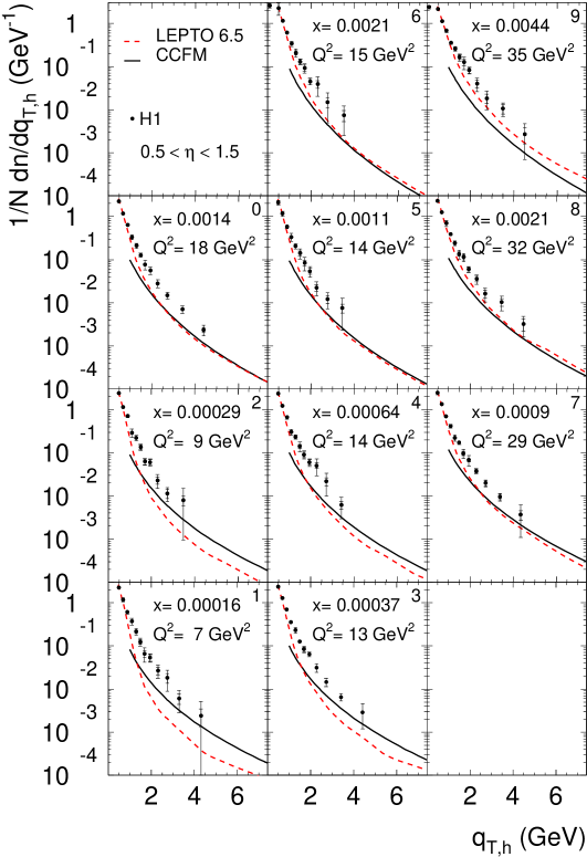
Figure 7: The charged hadron $k_{t}={q_{t,h}}$ spectrum in various bins of $x$ and $Q^{2}$ for $0.5<\eta_{\mbox{\scriptsize cms}}<1.5$. The data are from the H1 collaboration [29].

To avoid the problems associated with the $E_{t}$ flow, one should consider a measurement which concentrates on high-transverse momenta, and is consequently less sensitive to hadronisation and to the mistreatment of the emission of soft particles. Such an observable is the charged hadron transverse momentum ($q_{t,h}$) spectrum for a given rapidity. Since the one-particle inclusive cross section calculated in (13) is for emitted gluons, to allow a comparison with the data it is necessary to perform the convolution with the appropriate fragmentation function to obtain the spectrum for hadrons. The spectrum for a hadron of type $h$ is

$$\frac{dn}{d{q_{t,h}}\,d\eta}(x,Q^{2})=\left(\frac{d\sigma}{dx\,dQ^{2}}\right)^{-1}\int_{q_{t,h}}\frac{d{\bar{q}}_{t}}{{\bar{q}}_{t}}\,D^{h}_{g}({q_{t,h}}/{\bar{q}}_{t},{\bar{q}}_{t}^{2})\,\frac{d\sigma}{dx\,dQ^{2}\,d{\bar{q}}_{t}\,d\eta}\,.$$ (15)

We make the approximation that the direction of the resulting hadron is the same as that of the parent gluon and use the NLO fragmentation functions of Binnewies et al., as given in [46]. At our level of accuracy, it would have been equally valid to use the LO fragmentation functions.

We compare with the preliminary results from the H1 1994 data [29] in figure 7. At low transverse momenta the spectra that we obtain are much lower than the data — this is as expected given the lack of soft-radiation and hadronisation corrections discussed in the previous section.

For the large-$q_{t,h}$ part of the spectrum there is moderate agreement for a range of $x$ and $Q^{2}$ bins, though the CCFM results seem systematically low. At larger $x$ this can be explained by the fact that we are not counting the charged particles that come from the fragmentation of the quark box. At lower $x$ one can however say that the CCFM results are favoured compared to those from a DGLAP-based Monte Carlo event generator, such as LEPTO[47], though they are still not perfect.

The sensitivity of these results to the evolution parameters is moderate: altering $k_{0}$ by a factor of two (and the other fit parameters appropriately) affects the normalisation by about $25\%$.

5.3 Forward jets

Another quantity that is supposed to be particularly sensitive to small-$x$ dynamics is the forward-jet cross section, originally proposed in a slightly different form by Mueller and Navelet for proton-proton collisions [16] and then adapted to DIS [48, 49]. One of the main difficulties in obtaining a reliable prediction of this quantity is that experimentally one measures a jet, using a jet algorithm. The best that one can do with a one-particle-inclusive cross section is to associate with an emitted gluon a jet with the same energy and direction. This neglects the effect of multiple emission from the $t$-channel gluon, partonic showering and hadronisation, all of which play a role which varies according to the jet algorithm: as shown by the ZEUS collaboration [30], the choice of jet-algorithm can quite easily affect the results by about $15\%$. So in some sense this is the highest level of precision with which one can compare to a single-particle-inclusive approach with the data. Another element is that events in which 2 jets satisfy the selection cuts are treated differently experimentally (one counts only one of them), and one-particle-inclusively (one counts both of them) – however such events occur rarely ($2\%$ of the time in the ZEUS sample), and so this difference in treatment is of little practical importance.

In most forward-jet rate calculations, rather than using CCFM (or BFKL) evolution before the emission of the forward jet, as in (11), one uses DGLAP evolution (i.e. rather than ${\cal{B}}$ depending on ${\cal{A}}$, it depends on the normal DGLAP structure functions, $xg(x)$ and $xq(x)$). The motivations for using DGLAP evolution are that at relevant values of $x_{jet}$ (which can be of the order of $0.1$) one has a good knowledge of the DGLAP parton densities; our CCFM-based densities in that region may not be sufficiently constrained by the small-$x$ $F_{2}$ data, and in any case do not include quarks. On the other hand, with CCFM evolution one has the full $(k,p)$ dependence of the gluon density, whereas with DGLAP evolution this information must be added in.

To use the normal DGLAP structure functions before the emission, one follows exactly the same procedure as before, except that one replaces (11) with

$${\cal{B}}^{(\mathrm{DGLAP})}_{{\bar{q}}_{t}{\bar{\eta}}}(x,k,p)=\int_{x}^{1}\frac{dz}{z}\int\frac{d^{2}q}{\pi q^{2}}\,{\bar{\alpha}}_{\mbox{\scriptsize s}}\left(q_{t}\right)\;\frac{x}{z}F\left(\frac{x}{z},q_{t}^{2}\right)\delta^{2}({\vec{k}}+{\vec{q}}_{t})\\ \times\Delta(z,k,q)\;\Theta(p-zq)\;\delta({\bar{q}}_{t}-q_{t})\;\delta\left({\bar{\eta}}-\ln\frac{zq}{2xE_{p}}\right)\,,$$ (16)

with ${\vec{q}}_{t}=(1-z){\vec{q}}$ and

$$F(x,q_{t}^{2})=\left[g\left({x},q_{t}^{2}\right)+\frac{C_{F}}{C_{A}}\left(q(x,q_{t}^{2})+{\bar{q}}(x,q_{t}^{2})\right)\right],$$ (17)

where $g$ and $q$ are usual DGLAP parton densities in the proton (and the sum over flavours is implicit for the quark and antiquark densities). Fixing $k$ through $\delta^{2}({\vec{k}}+{\vec{q}}_{t})$ corresponds to the approximation of strong transverse-momentum ordering (which should be valid in the region of $x_{jet}$ of interest).

The cuts used for the forward-jet measurement tend to be considerably more complicated than for the energy-flow or particle spectra. As a result the simplest way to obtain a prediction is to use a Monte Carlo integration method which generates $x,Q^{2}$ values, a four vector for the forward gluon (or quark), and a corresponding weight. To these one applies the experimental cuts as if the forward parton were a jet, and finally adds the weights of the configurations that survive.

Figure 8: The forward-jet cross section, and the results of the ZEUS measurement [30]. The upper figure shows three different approaches to calculating the results using the CCFM equation, while the lower figure compares the CCFM results with other theoretical predictions [40, 50].

We will compare our calculations with the ZEUS measurement [30]. The cuts are: $0.00045<x<0.045$, $E_{t,jet}>5$ GeV, $0.5<E_{t,jet}^{2}/Q^{2}<2$, the energy of the scattered electron $E_{e^{\prime}}>10$ GeV, $y_{Bj}>0.1$, $\theta_{Jet}<8.5$ degrees, $x_{Jet}>0.036$, and the jet must be in the target hemisphere of the Breit frame.

Figure 8 shows the ZEUS results and a calculation which includes CCFM evolution both before and after the forward-jet emission. The CCFM cross section is consistently too low everywhere. In the higher-$x$ bins this is not unexpected since there are other mechanisms of importance there which are not being considered (e.g. the forward jet can come from one of the legs of the quark box). But at low $x$ it is more difficult to justify. To examine the degree of uncertainty on our result, we have tried to simulate the effect of hadronisation and “mis-reconstruction” from a jet algorithm by adding 1 GeV of transverse energy to all jets, while maintaining their rapidity. This has a greater effect at small $x$ than at larger $x$, due to the fact that the cut on $E_{t,jet}^{2}/Q^{2}$, in conjunction with the correlation between $x$ and $Q^{2}$ (the cut on $y_{Bj}$) causes jets in events with larger $x$ to have a larger transverse momentum and hence be less sensitive to hadronisation. The effect of this is not inconsistent with the ${\cal O}\left({15\%}\right)$ jet-algorithm dependence mentioned above. In any case it is not sufficient to bring the CCFM curves into agreement with the data. The use of the DGLAP distribution for the incoming partons, rather than the CCFM distribution, tends to lower the results — so that does not help either. Changing the parameter sets for the evolution also had little effect, affecting only moderately ($\sim 20\%$) the normalisation. We note that a similar calculation carried out with the cuts used by H1 also falls below their recent data [31].

For reference we include also a comparison of our results with those of [40], where a normal BFKL-based calculation of the forward-jet cross section was carried out: the data are considerably closer to the results of [40] than to ours. We have also included the results of a NLO calculation using MEPJET [50], as presented in the ZEUS forward-jet paper [30]. For this kind of observable NLO is the first order which contributes, so the fact that the CCFM-based results are above the MEPJET prediction is to be expected.

Why does the version of the CCFM equation that is being used here lead to forward-jet results which are not satisfactory? The forward-jet measurement that is used experimentally does not cast much light on this, in part because of the numerous cuts, which lead to correlations between $x$ and $E_{t,jet}$ and restrict the available $x$ range. So it is instructive to examine a forward-jet-like (where the forward-jet cannot come from the quark box) measurement which is free of these problems, such as

$$E_{t,jet}\,\frac{dF_{2}(x,Q^{2})}{d\eta\,dE_{t,jet}}\,,$$ (18)

as a function of $x$, for fixed $E_{t,jet}$, $Q^{2}$ and $\eta$. At very small $x$ we know that in the absence of small-$x$ evolution (the Born approximation) it should go to a constant, independent of $x$. So what we can do is compare the CCFM result for this quantity with a similar quantity worked out in the Born approximation, namely using

$$C^{(BORN)}_{{\bar{q}}_{t}{\bar{\eta}}}(x,k,p)=\int_{x}^{1}\frac{dz}{z}\int\frac{d^{2}q}{\pi q^{2}}\,{\bar{\alpha}}_{\mbox{\scriptsize s}}\left(q_{t}\right)\;\frac{x}{z}F\left(\frac{x}{z},q_{t}^{2}\right)\delta^{2}({\vec{k}}+{\vec{q}}_{t})\\ \times\Theta(p-zq)\;\delta({\bar{q}}_{t}-q_{t})\;\delta\left({\bar{\eta}}-\ln\frac{zq}{2xE_{p}}\right)\,.$$ (19)

The result is shown in figure 9.

Concentrating first on the Born result, we see that it takes a considerable range in $x$ to reach its constant value (bearing in mind that $x_{jet}\simeq 0.06$): assuming that the incoming gluon has transverse momentum $Q$, the kinematics of the quark box require the momentum fraction of the incoming gluon, $x_{g}$, to satisfy $x_{g}>2x_{Bj}$ — to obtain the full asymptotic cross section $x_{g}$ should be larger than that limit by an order of magnitude (the cross section goes as $dx_{g}/x_{g}^{2}$). But $x_{g}$ itself must satisfy $x_{g}\ll x_{jet}$ otherwise the cross section is sensitive to the DGLAP parton distributions at $x$ values larger than $x_{jet}$, and the gluon distribution drops quite fast with increasing $x$.

What is surprising is that the full CCFM result should drop below the Born result for such a considerable range in $x$, and only for $x<10^{-5}$ does it start to overtake the Born result: the CCFM evolution takes a long time to get started. This again is probably a consequence of the large virtual corrections, which can be compensated only when there is a sufficiently asymptotic gluon transverse-momentum distribution — and that which arises immediately after the forward-jet emission is far from asymptotic.

Figure 9: A “toy” forward jet measurement, comparing the result with evolution to that without evolution (Born). In both cases the input parton distribution is the DGLAP one.

6 Conclusions

The main aim of this paper has been to apply the angular ordered small-$x$ formalism, in the form of the CCFM equation, to the description of HERA data, with the purpose of determining whether, as it stands currently, it is suitable as a basis for quantitative phenomenology.

As a first step it was necessary to decide on the treatment of $1-z$ kinematical factors in the virtual corrections ($T=1$ or $T=1-z$, in (3)). The final choice was made on the basis that $T=1-z$ gives an asymptotic exponent which is considerably lower than $T=1$ and LL BFKL, and roughly in accord with phenomenological expectations and with first estimates from a partial resummation of NLL corrections to the BFKL equation. This choice does however have the property that its NLL corrections are four times larger than the true NLL corrections to the BFKL equation. The part of the splitting function which is finite as $z\to 0$ was left out, partly because it is not clear how it should be included, partly because whichever method of inclusion one chooses, there are considerable technical difficulties in its implementation. We will return to the discussion of these points shortly. To constrain the infra-red properties of the evolution, we used the $F_{2}$ structure function; we then examined some of the classic “BFKL” structure-function and final-state signals: $F_{2}^{c}$, $R$, the transverse energy flow, the charged hadron transverse momentum spectrum and the forward-jet cross section.

The transverse energy flow is much lower than the data, but this was to be expected: both the $z\to 0$ finite part of the splitting function and non-perturbative contributions are expected to give large (though formally subleading) contributions.

The failure to reproduce the forward-jet cross section data is less acceptable. An analysis of the problem indicates that after the emission of the forward jet, the small-$x$ evolution has a long period in which there is no growth of the cross section — non-asymptotic effects are important. The exact reason for this may well be connected with the non-trivial interplay between real and virtual contributions, which leads also to the large NLL corrections to the evolution. The importance of non-asymptotic effects may also be responsible for the lowness of the predictions for $F_{2}^{c}$ and the charged-particle transverse momentum spectra (though the results for the latter are better than those from DGLAP-based approaches, at least for some values of $x$ and $Q^{2}$).

It is interesting to note that the LDC model [35, 36] displays problems similar to those found here. The physics contained is somewhat different (e.g. the evolution is symmetric) but the general approach is somewhat similar — they too use a fit to the $F_{2}$ structure function as a constraint on the evolution parameters. The fit to the structure function data works well, but again a number of final state quantities are too low. It is not clear whether the problems in the LDC model are of the same nature as those in our CCFM implementation (i.e. due to non-asymptotic effects), but it might be a matter worthy of further investigation.

As a consequence of the problems described here, one is essentially led to rule out the CCFM equation with $T=1-z$ and without the $z\to 0$ finite part of the splitting function. It is tempting to suggest that we should have used $T=1$ and then included the $z\to 0$ finite part of the splitting function (in some arbitrary way). This would be the physics of SMALLX program — which so far has only been used for the study of final states in which the photon-gluon fusion produces charm quarks [34]. Since most final state studies at HERA do not select for the presence of open charm, there is relatively little data for comparison, so it would be worthwhile extending that study to the case with the full mix of quarks in the photon-gluon fusion.

In the longer term we need to work towards a theoretical approach free of the current ambiguities. Much of the basic information is probably already at our disposal, in the form of the NLL corrections to the BFKL kernel [8, 9]. We should be looking for an evolution equation which rather just than giving a “reasonable exponent” (a condition satisfied both by the LDC and by the form of the CCFM equation described in this paper), explicitly reproduces the structure of the NLL corrections (whether the part associated with symmetrisation, of with the $z\to 0$ finite part of the splitting function), and which resums these corrections in a sensible way. Of course it should also satisfy basic properties associated with coherence in the final state. Another important element lies in the calculation of the boson-gluon fusion hard matrix element to next-to-leading order. After the completion of such a programme we should be in a relatively strong position to carry out quantitatively meaningful BFKL phenomenology. It may take a while for such a stage to be reached — but in the mean time it is of paramount importance that experimental measurements of BFKL signals continue.

Appendix A Photon-gluon fusion

In this appendix we outline the calculation of the one-loop photon-gluon fusion hard matrix element. The results presented have been derived with the aid of the HIP package for Mathematica [51].

The starting point is the tree-level amplitude, coming from the diagrams illustrated in figure 10a:

$${\cal M}^{\mu\alpha} = -ie_{Q}g_{s}\,t^{a}\;\bar{u}(p_{1})\left[{\gamma^{\mu}\;[(p_{1}-q)\cdot\gamma+m]\;\gamma^{\alpha}\over t-m^{2}}+\right.$$

$$\left.{\gamma^{\alpha}\;[(p_{1}-k)\cdot\gamma+m]\;\gamma^{\mu}\over u-m^{2}}\right]v(p_{2})\;.$$

Here $e_{Q}$ is the fractional quark charge, $g_{s}$ is the strong coupling constant, $t^{a}$ are the SU(3) colour generators, $m$ is the quark mass, $p_{1}$ and $p_{2}$ are the outgoing quark and anti-quark momenta and $q$ and $k$ denote respectively the photon and gluon momenta. The Mandelstam variables are defined as $s=(k+q)^{2}$, $t=(q-p_{1})$ and $u=(q-p_{2})^{2}$.

Figure 10: a) The one loop diagrams contributing to photon gluon fusion vertex. b) The squared amplitude Lorentz indices.

The hard matrix tensor $H^{\mu{\mu^{\ast}},\alpha{\alpha^{\ast}}}$ is obtained by squaring the amplitude, averaging over the colour of the incoming gluon, summing over the final state (i.e. quark and anti-quark) degrees of freedom and integrating over the two-particle phase space $d\phi\,(p_{1},p_{2})$:

$$H^{\mu{\mu^{\ast}},\alpha{\alpha^{\ast}}}(q,k)=\int d\phi\,(p_{1},p_{2})\;\overline{\sum_{g}}\;\sum_{q,\bar{q}}{{\cal M}^{\mu\alpha}}^{\dagger}\!{\cal M}^{{\mu^{\ast}}{\alpha^{\ast}}}\,.$$ (21)

It depends only on the photon and gluon Lorentz indices and momenta (figure 10).

The “reduced cross section” ${\hat{\sigma}}_{F_{2}}$ appearing in (9) is then defined through

$${\hat{\sigma}}_{F_{i}}=\frac{k_{t}^{2}}{2x_{f}}\;\hat{w}_{i,\mu{\mu^{\ast}}}\;H^{\mu{\mu^{\ast}}\alpha{\alpha^{\ast}}}(q,k)\;\hat{P}_{{\scriptscriptstyle{BFKL}},\alpha{\alpha^{\ast}}}\;,$$ (22)

where the photon Lorentz indices are contracted over the usual projector used in DIS to extract the structure function $F_{2}$ and the longitudinal structure function $F_{L}$:

$$w_{2}^{\mu{\mu^{\ast}}} = {1\over p\cdot q}\left(p^{\mu}-{p\cdot q\over q^{2}}q^{\mu}\right)\left(p^{{\mu^{\ast}}}-{p\cdot q\over q^{2}}q^{{\mu^{\ast}}}\right)$$ (23)

$$w_{L}^{\mu{\mu^{\ast}}} = {1\over p\cdot q}\left[q^{2}\left(g^{\mu{\mu^{\ast}}}-{q^{\mu}q^{{\mu^{\ast}}}\over q^{2}}\right)-\left(p^{\mu}-{p\cdot q\over q^{2}}q^{\mu}\right)\left(p^{{\mu^{\ast}}}-{p\cdot q\over q^{2}}q^{{\mu^{\ast}}}\right)\right]$$ (24)

and the gluon Lorentz indices are contracted over the projector

$$\hat{P}_{{\scriptscriptstyle{BFKL}}}^{\alpha{\alpha^{\ast}}}=\left.\frac{k_{\perp}^{\alpha}k_{\perp}^{{\alpha^{\ast}}}}{-k^{2}_{\perp}}\right|_{k=x_{f}\,p+k_{\perp}}=\frac{x_{f}^{2}}{k_{t}^{2}}p^{\alpha}p^{{\alpha^{\ast}}}\;,$$ (25)

coming from the high energy (or $k_{t}$) factorisation prescription [37, 38, 39]. Additionally the prescription specifies that in (22), the incoming gluon momentum should be approximated by $k=x_{f}p+k_{\perp}$ with $p$ the hadron momentum, so that $k\cdot p=0$ and $k^{2}=k_{\perp}^{2}=-k_{t}^{2}$.

After the contractions with the two projectors, the reduced cross section acquires a dependence on the proton momentum (i.e. it is not just a function of the photon and gluon momenta), which complicates the phase-space integration for the outgoing quarks. As a result it seems very difficult to carry out this integration analytically, and the answer is usually left in the form of a Mellin transform, or of a double integral which must be evaluated numerically [37, 38, 39, 40, 41].

In this appendix we show that it is possible to carry out the phase space integration analytically, but this must be done before the contraction with the projectors. Accordingly, we expand $H^{\mu{\mu^{\ast}},\alpha{\alpha^{\ast}}}(q,k)$ over a tensor basis $\{T_{i}^{\mu{\mu^{\ast}},\alpha{\alpha^{\ast}}}(q,k)\}$, taking into account the symmetry of $H^{\mu{\mu^{\ast}},\alpha{\alpha^{\ast}}}$ with respect to both the $\mu,{\mu^{\ast}}$ and $\alpha,{\alpha^{\ast}}$ pair of indices, and its transversality with respect to $q$ and $k$ (i.e. $q_{\mu}H^{\mu{\mu^{\ast}},\alpha{\alpha^{\ast}}}=0$, $k_{\alpha}H^{\mu{\mu^{\ast}},\alpha{\alpha^{\ast}}}=0$).

First of all, let us introduce a four-dimensional basis $h_{i}^{\mu\nu}(a,b)$ for a two-index symmetric tensor which depends on two four-momenta $a$ and $b$:

$$h_{1}^{\mu\nu}(a,b) = -\left(g^{\mu\nu}-{a^{\mu}a^{\nu}\over a^{2}}\right)\,,$$

$$h_{2}^{\mu\nu}(a,b) = -{a^{2}\over\sqrt{(a\cdot b)^{2}-a^{2}b^{2}}}\left(b^{\mu}-{a\cdot b\over a^{2}}a^{\mu}\right)\left(b^{\nu}-{a\cdot b\over a^{2}}a^{\nu}\right)\,,$$

$$h_{3}^{\mu\nu}(a,b) = {a^{\mu}a^{\nu}\over a^{2}}\,,$$ (26)

$$h_{4}^{\mu\nu}(a,b) = {a^{\mu}b^{\nu}+b^{\mu}a^{\nu}\over a\cdot b}\,.$$

We then construct a basis $B_{i}^{\mu{\mu^{\ast}},\alpha{\alpha^{\ast}}}(q,k)$ for a four-index tensor which depends on the two momenta $q$ and $k$ and which is symmetric with respect to $\mu,{\mu^{\ast}}$ and to $\alpha,{\alpha^{\ast}}$. There are 21 such independent structures. Sixteen can be chosen as the products

$$B_{4(i-1)+j}^{\mu{\mu^{\ast}},\alpha{\alpha^{\ast}}}(q,k)=h_{i}^{\mu{\mu^{\ast}}}(q,k)\;h_{j}^{\alpha{\alpha^{\ast}}}(k,q)\,,\ \ \ \ i,j=1,\ldots,4\,,$$ (27)

while for the others we take

$$B_{17}^{\mu{\mu^{\ast}},\alpha{\alpha^{\ast}}}(q,k) = \left(g^{\mu\alpha}g^{{\mu^{\ast}}{\alpha^{\ast}}}+g^{\mu{\alpha^{\ast}}}g^{{\mu^{\ast}}\alpha}\right)\,,$$

$$B_{18}^{\mu{\mu^{\ast}},\alpha{\alpha^{\ast}}}(q,k) = \frac{1}{q^{2}}\left(g^{\mu\alpha}q^{\mu^{\ast}}q^{\alpha^{\ast}}+g^{\mu{\alpha^{\ast}}}q^{\mu^{\ast}}q^{\alpha}+g^{{\mu^{\ast}}\alpha}q^{\mu}q^{\alpha^{\ast}}+g^{{\mu^{\ast}}{\alpha^{\ast}}}q^{\mu}q^{\alpha}\right)\,,$$

$$B_{19}^{\mu{\mu^{\ast}},\alpha{\alpha^{\ast}}}(q,k) = \frac{1}{k^{2}}\left(g^{\mu\alpha}k^{\mu^{\ast}}k^{\alpha^{\ast}}+g^{\mu{\alpha^{\ast}}}k^{\mu^{\ast}}k^{\alpha}+g^{{\mu^{\ast}}\alpha}k^{\mu}k^{\alpha^{\ast}}+g^{{\mu^{\ast}}{\alpha^{\ast}}}k^{\mu}k^{\alpha}\right)\,,$$ (28)

$$B_{20}^{\mu{\mu^{\ast}},\alpha{\alpha^{\ast}}}(q,k) = \frac{1}{q\cdot k}\left(g^{\mu\alpha}q^{\mu^{\ast}}k^{\alpha^{\ast}}+g^{\mu{\alpha^{\ast}}}q^{\mu^{\ast}}k^{\alpha}+g^{{\mu^{\ast}}\alpha}q^{\mu}k^{\alpha^{\ast}}+g^{{\mu^{\ast}}{\alpha^{\ast}}}q^{\mu}k^{\alpha}\right)\,,$$

$$B_{21}^{\mu{\mu^{\ast}},\alpha{\alpha^{\ast}}}(q,k) = \frac{1}{q\cdot k}\left(g^{\mu\alpha}k^{\mu^{\ast}}q^{\alpha^{\ast}}+g^{\mu{\alpha^{\ast}}}k^{\mu^{\ast}}q^{\alpha}+g^{{\mu^{\ast}}\alpha}k^{\mu}q^{\alpha^{\ast}}+g^{{\mu^{\ast}}{\alpha^{\ast}}}k^{\mu}q^{\alpha}\right)\,,$$

Since $H^{\mu{\mu^{\ast}},\alpha{\alpha^{\ast}}}(q,k)$ is explicitly transverse with respect to both $q$ and $k$, let us now concentrate on the set of symmetric tensors $T_{i}^{\mu{\mu^{\ast}},\alpha{\alpha^{\ast}}}=\sum_{j=1}^{21}C_{ij}B_{j}^{\mu{\mu^{\ast}},\alpha{\alpha^{\ast}}}$ that satisfy $q_{\mu}T_{i}^{\mu{\mu^{\ast}},\alpha{\alpha^{\ast}}}=0$ and $k_{\alpha}T_{i}^{\mu{\mu^{\ast}},\alpha{\alpha^{\ast}}}=0$. There are 6 such independent tensors, specified by

$$C^{T}=\left(\begin{array}[]{cccccc}{3\over 2}-{1\over 4\rho}&{1\over 4\rho}&{1\over 4\rho}&{{-1}\over 4\rho}&{1\over{2\rho}}&{{-1}\over 4\rho}\\ {1\over 2}-{1\over 4\rho}&1+{1\over 4\rho}&{1\over 4\rho}&{{-1}\over 4\rho}&{1\over{2\rho}}&{{-1}\over 4\rho}\\ 0&0&0&0&0&0\\ 0&0&0&0&0&0\\ {1\over 2}-{1\over 4\rho}&{1\over 4\rho}&1+{1\over 4\rho}&{{-1}\over 4\rho}&{1\over{2\rho}}&{{-1}\over 4\rho}\\ {1\over 2}+{1\over{2\rho^{2}}}+{3\over 4\rho}&{{-\left(2+7\rho\right)}\over{4\rho^{2}}}&{{-\left(2+7\rho\right)}\over{4\rho^{2}}}&1+{1\over{2\rho^{2}}}+{7\over 4\rho}&{{-\left(2+3\rho\right)}\over{2\rho^{2}}}&{{2-\rho}\over{4\rho^{2}}}\\ -1+{1\over{2\rho^{2}}}+{3\over{2\rho}}&{{-\left(1+5\rho\right)}\over{2\rho^{2}}}&{{-\left(1+5\rho\right)}\over{2\rho^{2}}}&{{1+5\rho}\over{2\rho^{2}}}&{{-1-3\rho}\over{\rho^{2}}}&{{1+\rho}\over{2\rho^{2}}}\\ {{-1}\over{2\rho^{2}}}&{1\over{2\rho^{2}}}+{1\over{\rho}}&{1\over{2\rho^{2}}}+{1\over{\rho}}&{{-1}\over{2\rho^{2}}}-{1\over{\rho}}&{{1+\rho}\over{\rho^{2}}}&{{-1}\over{2\rho^{2}}}\\ 0&0&0&0&0&0\\ -1+{1\over{2\rho^{2}}}+{3\over{2\rho}}&{{-\left(1+5\rho\right)}\over{2\rho^{2}}}&{{-\left(1+5\rho\right)}\over{2\rho^{2}}}&{{1+5\rho}\over{2\rho^{2}}}&{{-1-3\rho}\over{\rho^{2}}}&{{1+\rho}\over{2\rho^{2}}}\\ {{-1-3\rho+2\rho^{2}}\over{2(\rho-1)\rho^{2}}}&{{1+5\rho}\over{2(\rho-1)\rho^{2}}}&{{1+5\rho}\over{2(\rho-1)\rho^{2}}}&{{1+5\rho}\over{2(1-\rho)\rho^{2}}}&{{1+3\rho}\over{(\rho-1)\rho^{2}}}&{{1+\rho}\over{2(1-\rho)\rho^{2}}}\\ {1\over{2(\rho-1)\rho^{2}}}&{{1+2\rho}\over{2(1-\rho)\rho^{2}}}&{{1+2\rho}\over{2(1-\rho)\rho^{2}}}&{{1+2\rho}\over{2(\rho-1)\rho^{2}}}&{{1+\rho}\over{\rho^{2}-{{\rho}^{3}}}}&{1\over{2(\rho-1)\rho^{2}}}\\ 0&0&0&0&0&0\\ {{-1}\over{2\rho^{2}}}&{1\over{2\rho^{2}}}+{1\over{\rho}}&{1\over{2\rho^{2}}}+{1\over{\rho}}&{{-1}\over{2\rho^{2}}}-{1\over{\rho}}&{{1+\rho}\over{\rho^{2}}}&{{-1}\over{2\rho^{2}}}\\ {1\over{2(\rho-1)\rho^{2}}}&{{1+2\rho}\over{2(1-\rho)\rho^{2}}}&{{1+2\rho}\over{2(1-\rho)\rho^{2}}}&{{1+2\rho}\over{2(\rho-1)\rho^{2}}}&{{1+\rho}\over{\rho^{2}-{{\rho}^{3}}}}&{1\over{2(\rho-1)\rho^{2}}}\\ {{-2+3\rho-2\rho^{2}}\over{4(\rho-1)\rho^{2}}}&{{2+\rho}\over{4(\rho-1)\rho^{2}}}&{{2+\rho}\over{4(\rho-1)\rho^{2}}}&{{2+\rho}\over{4(1-\rho)\rho^{2}}}&{1\over{(\rho-1)\rho^{2}}}&{{-2+\rho}\over{4(\rho-1)\rho^{2}}}\\ -{1\over 2}+{1\over 4\rho}&{{-1}\over 4\rho}&{{-1}\over 4\rho}&{1\over 4\rho}&{{-1}\over{2\rho}}&{1\over 4\rho}\\ {{-3+2\rho}\over{4(\rho-1)}}&{3\over{4(\rho-1)}}&{3\over{4(\rho-1)}}&{3\over{4-4\rho}}&{1\over{-1+\rho}}&{1\over{4-4\rho}}\\ {{-3+2\rho}\over{4(\rho-1)}}&{3\over{4(\rho-1)}}&{3\over{4(\rho-1)}}&{3\over{4-4\rho}}&{1\over{-1+\rho}}&{1\over{4-4\rho}}\\ {{-3+2\rho}\over{4\rho-4\rho^{2}}}&{3\over{4\rho-4\rho^{2}}}&{3\over{4\rho-4\rho^{2}}}&{3\over{-4\rho+4\rho^{2}}}&{1\over{\rho-\rho^{2}}}&-{1\over{4\rho-4\rho^{2}}}\\ {1\over{-4\rho+4\rho^{2}}}&{{1+2\rho}\over{4\rho-4\rho^{2}}}&{{1+2\rho}\over{4\rho-4\rho^{2}}}&{{1+2\rho}\over{-4\rho+4\rho^{2}}}&{{1+\rho}\over{2\rho-2\rho^{2}}}&-{1\over{4\rho-4\rho^{2}}}\end{array}\right)$$ (29)

with $\rho=\frac{k^{2}q^{2}}{(k\cdot q)^{2}}$.

This choice has the advantage that the corresponding “projectors” $\{\hat{T}_{i,\mu{\mu^{\ast}},\alpha{\alpha^{\ast}}}(q,k)\}$, which satisfy the relations $\hat{T}_{i,\mu{\mu^{\ast}},\alpha{\alpha^{\ast}}}\;T_{j}^{\mu{\mu^{\ast}},\alpha{\alpha^{\ast}}}=\delta_{ij}$, have straightforward forms:

$$\hat{T}_{1}^{\mu{\mu^{\ast}},\alpha{\alpha^{\ast}}} = \frac{1}{4}\left(g^{\mu{\mu^{\ast}}}+{{q^{2}k^{\mu}k^{\mu^{\ast}}}\over{(k\cdot q)^{2}-k^{2}q^{2}}}\right)\left(g^{\alpha{\alpha^{\ast}}}+{{k^{2}q^{\alpha}q^{\alpha^{\ast}}}\over{(k\cdot q)^{2}-k^{2}q^{2}}}\right)\,,$$

$$\hat{T}_{2}^{\mu{\mu^{\ast}},\alpha{\alpha^{\ast}}} = \frac{1}{4}\left(g^{\mu{\mu^{\ast}}}+{{q^{2}k^{\mu}k^{\mu^{\ast}}}\over{(k\cdot q)^{2}-k^{2}q^{2}}}\right)\left(g^{\alpha{\alpha^{\ast}}}+{{3k^{2}q^{\alpha}q^{\alpha^{\ast}}}\over{(k\cdot q)^{2}-k^{2}q^{2}}}\right)\,,$$

$$\hat{T}_{3}^{\mu{\mu^{\ast}},\alpha{\alpha^{\ast}}} = \frac{1}{4}\left(g^{\mu{\mu^{\ast}}}+{{3q^{2}k^{\mu}k^{\mu^{\ast}}}\over{(k\cdot q)^{2}-k^{2}q^{2}}}\right)\left(g^{\alpha{\alpha^{\ast}}}+{{k^{2}q^{\alpha}q^{\alpha^{\ast}}}\over{(k\cdot q)^{2}-k^{2}q^{2}}}\right)\,,$$

$$\hat{T}_{4}^{\mu{\mu^{\ast}},\alpha{\alpha^{\ast}}} = \frac{1}{4}\left(g^{\mu{\mu^{\ast}}}+{{3q^{2}k^{\mu}k^{\mu^{\ast}}}\over{(k\cdot q)^{2}-k^{2}q^{2}}}\right)\left(g^{\alpha{\alpha^{\ast}}}+{{3k^{2}q^{\alpha}q^{\alpha^{\ast}}}\over{(k\cdot q)^{2}-k^{2}q^{2}}}\right)\,,$$ (30)

$$\hat{T}_{5}^{\mu{\mu^{\ast}},\alpha{\alpha^{\ast}}} = {k^{2}q^{2}\over 4(k\cdot q)[(k\cdot q)^{2}-k^{2}q^{2}]}\left(g^{{\alpha^{\ast}}{\mu^{\ast}}}k^{\mu}q^{\alpha}+g^{\mu{\alpha^{\ast}}}k^{\mu^{\ast}}q^{\alpha}+g^{\alpha{\mu^{\ast}}}k^{\mu}q^{\alpha^{\ast}}+g^{\alpha\mu}k^{\mu^{\ast}}q^{\alpha^{\ast}}\right)\,,$$

$$\hat{T}_{6}^{\mu{\mu^{\ast}},\alpha{\alpha^{\ast}}} = {k^{2}q^{2}\over 2(k\cdot q)^{2}}\left(g^{\alpha{\mu^{\ast}}}g^{\mu{\alpha^{\ast}}}+g^{\alpha\mu}g^{{\alpha^{\ast}}{\mu^{\ast}}}\right)\,.$$

We then write the decomposition

$$H^{\mu{\mu^{\ast}},\alpha{\alpha^{\ast}}}=\sum_{i=1}^{6}H_{i}T_{i}^{\mu{\mu^{\ast}},\alpha{\alpha^{\ast}}}\,,$$ (31)

where the coefficients $H_{i}$ are

$$H_{i}=\hat{T}_{i,\mu{\mu^{\ast}},\alpha{\alpha^{\ast}}}\;H^{\mu{\mu^{\ast}},\alpha{\alpha^{\ast}}}.$$ (32)

Since the $H_{i}$ depend only on $k$ and $q$, there exists a frame, namely the photon-gluon centre of mass frame, in which the quark-antiquark phase-space integration can be performed analytically without difficulty. This would not have been the case if we had already contracted with the photon and gluon projectors, as these would have introduced a non-trivial dependence on an additional external momentum (that of the proton). Our results for the coefficients $H_{i}$ are:

$$H_{i} = \alpha_{\mbox{\scriptsize s}}e_{Q}^{2}\left[\bar{H}^{(a)}_{i}+\bar{H}^{(b)}_{i}{4m^{2}J^{2}\over sk^{2}q^{2}+4m^{2}J^{2}}+\right.$$ (33)

$$+ \left.\bar{H}^{(c)}_{i}{J\over 4(k\cdot q)}\log{(k\cdot q)+J\sqrt{1-{4m^{2}\over s}}\over(k\cdot q)-J\sqrt{1-{4m^{2}\over s}}}\right]$$

where $J=\sqrt{(k\cdot q)^{2}-k^{2}q^{2}}$ and

$$\bar{H}^{(a)}_{1} = {\sqrt{1-{4m^{2}\over s}}\over J^{2}}\left(-2J^{2}-k^{2}s-q^{2}s-{{3k^{2}q^{2}s^{2}}\over{4J^{2}}}\right)\,,$$

$$\bar{H}^{(a)}_{2} = {\sqrt{1-{4m^{2}\over s}}\over J^{2}}\left(-2J^{2}-2k^{2}s-2q^{2}s-{{9k^{2}q^{2}s^{2}}\over{4J^{2}}}\right)\,,$$

$$\bar{H}^{(a)}_{3} = {\sqrt{1-{4m^{2}\over s}}\over J^{2}}\left(-2J^{2}-2k^{2}s-2q^{2}s-{{9k^{2}q^{2}s^{2}}\over{4J^{2}}}\right)\,,$$

$$\bar{H}^{(a)}_{4} = {\sqrt{1-{4m^{2}\over s}}\over J^{2}}\left(-2J^{2}-3k^{2}s-3q^{2}s-{{27k^{2}q^{2}s^{2}}\over{4J^{2}}}\right)\,,$$ (34)

$$\bar{H}^{(a)}_{5} = -{4\sqrt{1-{4m^{2}\over s}}k^{2}q^{2}s\over J^{2}(k\cdot q)}\,,$$

$$\bar{H}^{(a)}_{6} = -{8\sqrt{1-{4m^{2}\over s}}k^{2}q^{2}\over(k\cdot q)^{2}}\,,$$

and

$$\bar{H}^{(b)}_{1} = {\sqrt{1-{4m^{2}\over s}}\over J^{2}}\left(J^{2}-m^{2}s-{k^{2}q^{2}s^{2}\over 4J^{2}}\right)\,,$$

$$\bar{H}^{(b)}_{2} = {\sqrt{1-{4m^{2}\over s}}\over J^{2}}\left(J^{2}-m^{2}s+q^{2}s-{k^{2}q^{2}s^{2}\over 4J^{2}}\right)\,,$$

$$\bar{H}^{(b)}_{3} = {\sqrt{1-{4m^{2}\over s}}\over J^{2}}\left(J^{2}+k^{2}s-m^{2}s-{k^{2}q^{2}s^{2}\over 4J^{2}}\right)\,,$$ (35)

$$\bar{H}^{(b)}_{4} = {\sqrt{1-{4m^{2}\over s}}\over J^{2}}\left(J^{2}+k^{2}s-m^{2}s+q^{2}s+{3k^{2}q^{2}s^{2}\over 4J^{2}}\right)\,,$$

$$\bar{H}^{(b)}_{5} = {\sqrt{1-{4m^{2}\over s}}k^{2}q^{2}s^{2}\over J^{4}}\,,$$

$$\bar{H}^{(b)}_{6} = {\sqrt{1-{4m^{2}\over s}}k^{2}q^{2}\left(2J^{2}-4m^{2}s+s^{2}\right)\over J^{2}(k\cdot q)^{2}}\,,$$

and

$$\bar{H}^{(c)}_{1} = {1\over 2J^{6}}\Big{[}8J^{4}(k\cdot q)^{2}-8J^{4}(k\cdot q)s-8J^{2}(k\cdot q)k^{2}q^{2}s+4J^{4}s^{2}+$$

$$+ 6J^{2}k^{2}q^{2}s^{2}+3k^{4}q^{4}s^{2}+8J^{2}m^{2}\left(-2J^{2}m^{2}+(k\cdot q)^{2}s\right)\Big{]}\,,$$

$$\bar{H}^{(c)}_{2} = {1\over 2J^{6}}\Big{[}8J^{4}(k\cdot q)^{2}-8J^{4}(k\cdot q)s-16J^{2}(k\cdot q)k^{2}q^{2}s+4J^{4}s^{2}+$$

$$+ 14J^{2}k^{2}q^{2}s^{2}+9k^{4}q^{4}s^{2}+8J^{2}m^{2}\left(2J^{2}k^{2}-2J^{2}m^{2}-J^{2}s+2(k\cdot q)^{2}s\right)\Big{]}\,,$$

$$\bar{H}^{(c)}_{3} = {1\over 2J^{6}}\Big{[}8J^{4}(k\cdot q)^{2}-8J^{4}(k\cdot q)s-16J^{2}(k\cdot q)k^{2}q^{2}s+4J^{4}s^{2}+$$

$$+ 14J^{2}k^{2}q^{2}s^{2}+9k^{4}q^{4}s^{2}+8J^{2}m^{2}\left(-2J^{2}m^{2}+2J^{2}q^{2}-J^{2}s+2(k\cdot q)^{2}s\right)\Big{]}\,,$$

$$\bar{H}^{(c)}_{4} = {1\over 2J^{6}}\Big{[}8J^{4}(k\cdot q)^{2}-8J^{4}(k\cdot q)s-24J^{2}(k\cdot q)k^{2}q^{2}s+4J^{4}s^{2}+$$

$$+ 30J^{2}k^{2}q^{2}s^{2}+27k^{4}q^{4}s^{2}+8J^{2}m^{2}\left(-4J^{2}(k\cdot q)-2J^{2}m^{2}+3(k\cdot q)^{2}s\right)\Big{]}\,,$$

$$\bar{H}^{(c)}_{5} = {8k^{2}q^{2}s\over J^{4}}((k\cdot q)-m^{2})\,,$$

$$\bar{H}^{(c)}_{6} = {8k^{2}q^{2}\over J^{2}(k\cdot q)^{2}}[J^{2}+2k^{2}q^{2}+(k\cdot q)s+m^{2}\left(s-4(k\cdot q)-4m^{2}\right)]\,.$$

Though individually, each of the $\bar{H}$ suffer from a singularity at $J=0$, the results for the reduced cross sections are finite at $J=0$, and are given by:

$${\hat{\sigma}}_{F_{i}}\left(z,k_{t}^{2},Q^{2},m^{2}\right)={\alpha_{\mbox{\scriptsize s}}e_{Q}^{2}\over 8}\frac{1}{z}k_{t}^{2}\bar{\sigma}_{i}\left(Q^{2}(\frac{1}{z}-1)-k_{t}^{2},-k_{t}^{2},-Q^{2},m^{2}\right)\,,$$ (37)

with

$$\bar{\sigma}_{i}(s,k^{2},q^{2},m^{2}) = \left({q^{2}\over 2J^{2}}\right)^{2}\left[\;h^{(a)}_{i}+h^{(b)}_{i}{4m^{2}J^{2}\over sk^{2}q^{2}+4m^{2}J^{2}}+\right.$$ (38)

$$+ \left.(h^{(c)}_{i}+h^{(d)}_{i}){J\over 4(k\cdot q)}\log{(k\cdot q)+J\sqrt{1-{4m^{2}\over s}}\over(k\cdot q)-J\sqrt{1-{4m^{2}\over s}}}\;\right]\,,$$

where

$$h^{(a)}_{2} = {\sqrt{1-{4m^{2}\over s}}\over 2J^{4}}\Big{[}-32J^{6}-72J^{4}k^{2}q^{2}+96J^{4}(k\cdot q)s+$$

$$+360J^{2}(k\cdot q)k^{2}q^{2}s-48J^{4}s^{2}-330J^{2}k^{2}q^{2}s^{2}-315k^{4}q^{4}s^{2}\Big{]}\,,$$

$$h^{(b)}_{2} = {\sqrt{1-{4m^{2}\over s}}\over 2J^{4}}\Big{[}16J^{6}+24J^{4}k^{2}q^{2}-32J^{4}(k\cdot q)s-16J^{4}m^{2}s-48J^{2}(k\cdot q)k^{2}q^{2}s+$$ (39)

$$-36J^{2}k^{2}m^{2}q^{2}s+16J^{4}s^{2}+36J^{2}k^{2}q^{2}s^{2}+15k^{4}q^{4}s^{2}\Big{]}\,,$$

$$h^{(c)}_{2} = {1\over J^{6}}\Big{[}32{J^{8}}+80J^{6}k^{2}q^{2}+72J^{4}k^{4}q^{4}-32J^{6}(k\cdot q)s-336J^{4}(k\cdot q)k^{2}q^{2}s+$$

$$-360J^{2}(k\cdot q)k^{4}q^{4}s+16J^{6}s^{2}+240J^{4}k^{2}q^{2}s^{2}+540J^{2}k^{4}q^{4}s^{2}+315k^{6}q^{6}s^{2}\Big{]}\,,$$

$$h^{(d)}_{2} = {8m^{2}\over J^{4}}\Big{[}-16J^{4}(k\cdot q)-8J^{4}m^{2}-36J^{2}(k\cdot q)k^{2}q^{2}-18J^{2}k^{2}m^{2}q^{2}+12J^{4}s+$$

$$+60J^{2}k^{2}q^{2}s+45k^{4}q^{4}s\Big{]}\,,$$

and

$$h^{(a)}_{L} = {\sqrt{1-{4m^{2}\over s}}\over J^{4}}\Big{[}-24J^{4}k^{2}q^{2}+16J^{4}(k\cdot q)s+$$

$$+120J^{2}(k\cdot q)k^{2}q^{2}s-8J^{4}s^{2}-110J^{2}k^{2}q^{2}s^{2}-105k^{4}q^{4}s^{2}\Big{]}\,,$$

$$h^{(b)}_{L} = {\sqrt{1-{4m^{2}\over s}}k^{2}\over J^{4}}\Big{[}8J^{4}q^{2}+8J^{4}s+8J^{2}k^{2}q^{2}s-12J^{2}m^{2}q^{2}s+8J^{2}q^{4}s+$$ (40)

$$+8J^{2}q^{2}s^{2}+5k^{2}q^{4}s^{2}\Big{]}\,,$$

$$h^{(c)}_{L} = {2k^{2}q^{2}\over J^{6}}\Big{[}16J^{6}+24J^{4}k^{2}q^{2}-96J^{4}(k\cdot q)s-120J^{2}(k\cdot q)k^{2}q^{2}s+$$

$$+72J^{4}s^{2}+180J^{2}k^{2}q^{2}s^{2}+105k^{4}q^{4}s^{2}\Big{]}\,,$$

$$h^{(d)}_{L} = {16m^{2}q^{2}\over J^{4}}\Big{[}4J^{4}-12J^{2}(k\cdot q)k^{2}-6J^{2}k^{2}m^{2}+$$

$$+18J^{2}k^{2}s+15k^{4}q^{2}s\Big{]}\,.$$

References

-
[1]
V.N. Gribov and L.N. Lipatov, Sov. J. Nucl. Phys. 15 (1972) 438;
G. Altarelli and G. Parisi, Nucl. Phys. B 126 (1977) 298;
Yu.L. Dokshitzer, Sov. Phys. JETP 46 (1977) 641. -
[2]
L.N. Lipatov, Sov. J. Phys. 23 (1976) 338;
E.A. Kuraev, L.N. Lipatov and V.S. Fadin, Sov. Phys. JETP 45 (1977) 199;
Ya. Balitskii and L.N. Lipatov, Sov. J. Nucl. Phys. 28 (1978) 822. - [3] H1 Collaboration (S. Aid et al.), Nucl. Phys. B 470 (1996) 3 [hep-ex/9603004].
- [4] ZEUS Collaboration (M. Derrick et al.), Z. Physik C 72 (1996) 399 [hep-ex/9607002].
- [5] A.D. Martin, R.G Roberts, W.J. Stirling and R.S. Thorne, hep-ph/9805205.
- [6] M. Gluck, E. Reya and A. Vogt, Eur. Phys. J. C 5 (1998) 461 [hep-ph/9806404].
- [7] S. Forte and R.D. Ball, proceedings of International Workshop on Deep Inelastic Scattering and Related Phenomena (DIS 96), Rome, 1996, p. 208 [hep-ph/9607289].
-
[8]
L.N. Lipatov and V.S. Fadin, Sov. J. Nucl. Phys. 50 (1989) 712;
V.S. Fadin, R. Fiore and M.I. Kotsky, Phys. Lett. B 539 (1995) 181;
V.S. Fadin, R. Fiore and M.I. Kotsky, Phys. Lett. B 387 (1996) 593 [hep-ph/9605357];
V.S. Fadin, and L.N. Lipatov, Nucl. Phys. B 406 (1993) 259;
V.S. Fadin, R. Fiore and A. Quartarolo, Phys. Rev. D 50 (1994) 5893 [hep-th/9405127];
V.S. Fadin, R. Fiore, and M.I. Kotsky, Phys. Lett. B 389 (1996) 737 [hep-ph/9608229];
V.S. Fadin and L.N. Lipatov, Nucl. Phys. B 477 (1996) 767 [hep-ph/9602287];
V.S. Fadin, M. I. Kotsky and L.N. Lipatov, Phys. Lett. B 415 (1997) 97;
S. Catani, M. Ciafaloni and F.Hautman, Phys. Lett. B 242 (1990) 97;
S. Catani, M. Ciafaloni and F.Hautman, Nucl. Phys. B 366 (1991) 135;
V.S. Fadin, R. Fiore, A. Flashi, and M.I. Kotsky, Phys. Lett. B 422 (1998) 287 [hep-ph/9711427];
V. Del Duca, Phys. Rev. D 54 (1996) 989;
V. Del Duca, Phys. Rev. D 54 (1996) 4474;
V. Del Duca and C.R. Schmidt, Phys. Rev. D 57 (1998) 4069 [hep-ph/9711309];
V. Del Duca and C.R. Schmidt, hep-ph/9810215. -
[9]
M. Ciafaloni and G. Camici, Phys. Lett. B 430 (1998) 127
[hep-ph/9803389];
M. Ciafaloni, Phys. Lett. B 429 (1998) 349 [hep-ph/9801322];
M. Ciafaloni and G. Camici, Phys. Lett. B 412 (1997) 396 [hep-ph/9707390];
V.S. Fadin and L.N. Lipatov, Phys. Lett. B 429 (1998) 127 [hep-ph/9802290]. -
[10]
D.A. Ross, Phys. Lett. B 431 (1998) 161 [hep-ph/9804332];
E. Levin, hep-ph/9806228. - [11] J. Bartels, H. Lotter and M. Vogt Phys. Lett. B 373 (1996) 215.
- [12] A.H. Mueller, Phys. Lett. B 396 (1997) 251 [hep-ph/9612251].
- [13] G. Camici and M. Ciafaloni, Phys. Lett. B 395 (1997) 118 [hep-ph/9612235].
- [14] G.P. Salam, J. High Energy Phys. 07 (1998) 019 [hep-ph/9806482].
-
[15]
R.K. Ellis, Z. Kunszt and E.M. Levin,
Nucl. Phys. B 420 (1994) 517;
R.K. Ellis, F. Hautmann and B.R. Webber, Phys. Lett. B 348 (1995) 582 [hep-ph/9501307];
R.D. Ball and S. Forte, Phys. Lett. B 351 (1995) 313 [hep-ph/9501231]. - [16] A.H. Mueller and H. Navelet, Nucl. Phys. B 282 (1987) 727.
-
[17]
A.H. Mueller, Phys. Lett. B 104 (1981) 161;
B.I. Ermolaev and V.S. Fadin, Sov. Phys. JETP Lett. 33 (1981) 285;
Yu.L. Dokshitzer, V.S. Fadin and V.A. Khoze, Z. Physik C 15 (1982) 325;
A. Bassetto, M. Ciafaloni and G. Marchesini and A.H. Mueller, Nucl. Phys. B 207 (1982) 189;
A. Bassetto, M. Ciafaloni and G. Marchesini, Phys. Rept. 100 (1983) 201;
Yu.L. Dokshitzer, V.A. Khoze, S.I. Troyan and A.H. Mueller, Basics of Perturbative QCD, Editions Frontieres, Paris, France 1991. -
[18]
Yu.L. Dokshitzer, L.V. Gribov, V.A. Khoze and
S.I. Troyan, Phys. Lett. B 202 (1988) 276;
L.V. Gribov, Yu.L. Dokshitzer, V.A. Khoze and S.I. Troyan, Sov. Phys. JETP 67 (1988) 1303;
M. Ciafaloni, A. Bassetto, G. Marchesini, Phys. Rept. 100 (1983) 201. -
[19]
M. Ciafaloni, Nucl. Phys. B 296 (1987) 249;
S. Catani, F. Fiorani and G. Marchesini, Phys. Lett. B 234 (1990) 339;
S. Catani, F. Fiorani and G. Marchesini, Nucl. Phys. B 336 (1990) 18. - [20] G. Marchesini, Nucl. Phys. B 445 (1995) 40 [hep-ph/9412327].
- [21] G. Bottazzi, G. Marchesini, G.P. Salam and M. Scorletti, Nucl. Phys. B 505 (1997) 366 [hep-ph/9702418].
- [22] M. Ryskin, private communication.
-
[23]
L.H. Orr and W.J. Stirling, Phys. Rev. D 56 (1997) 5875
[hep-ph/9804331];
L.H. Orr and W.J. Stirling, Phys. Lett. B 436 (1998) 372 [hep-ph/9806371]. - [24] J.R. Forshaw and A. Sabio Vera, Phys. Lett. B 440 (1998) 141 [hep-ph/9806394].
- [25] B.R. Webber, Phys. Lett. B 444 (1998) 81 [hep-ph/9810286].
- [26] G.P. Salam, in preparation.
- [27] S. Catani,G. Marchesini and B.R. Webber, in preparation.
- [28] H1 collaboration, contrib. paper pa02-073 to ICHEP’96, Warsaw 1996.
- [29] H1 collaboration (C. Adloff et al.), Nucl. Phys. B 485 (1997) 3 [hep-ex/9610006].
- [30] ZEUS Collaboration (J. Breitweg et al.), hep-ex/9805016.
- [31] H1 Collaboration (C. Adloff et al.), hep-ex/9809028.
- [32] J. Kwiecinski, A.D. Martin and P.J. Sutton, Phys. Rev. D 53 (1996) 6094 [hep-ph/9511263].
- [33] G. Marchesini and B.R. Webber, Nucl. Phys. B 386 (1992) 215.
- [34] K. Golec-Biernat, L. Goerlich and J. Turnau, Nucl. Phys. B 527 (1998) 289 [hep-ph/9712345].
- [35] B. Andersson, G. Gustafson, J. Samuelsson, Nucl. Phys. B 467 (1996) 443.
- [36] H. Kharraziha and L. Lönnblad, J. High Energy Phys. 03 (1998) 006 [hep-ph/9709424]. Phys. Rev. D 53 (1996) 6094 [hep-ph/9511263].
- [37] S. Catani, M. Ciafaloni and F. Hautmann, Nucl. Phys. B 366 (1991) 135.
- [38] J.C. Collins and R.K. Ellis, Nucl. Phys. B 360 (1991) 3.
- [39] E.M.Levin, M.G. Ryskin, Yu.M. Shabelskii and A.G. Shuvaev, Sov. J. Nucl. Phys. 53 (1991) 657.
-
[40]
J. Bartels, V. Del Duca, A. De Roeck, D. Graudenz,
and M. Wüsthoff, Phys. Lett. B 384 (1996) 300;
J. Bartels, V. Del Duca and M. Wüsthoff, Z. Physik C 76 (1997) 75. - [41] J. Kwiecinski, S.C. Lang and A.D. Martin, Eur. Phys. J. C 6 (1999) 671 [hep-ph/9707240].
- [42] H1 Collaboration (Adloff et al.), Z. Physik C 72 (1996) 593 [hep-ex/9607012].
- [43] ZEUS Collaboration (Breitweg et al.) Phys. Lett. B 407 (1997) 402 [hep-ex/9706009].
- [44] H. Navelet, R. Peschanski, C. Royon and S. Wallon, Phys. Lett. B 385 (1996) 357, [hep-ph/9605389].
- [45] Yu.L. Dokshitzer and B.R. Webber, Phys. Lett. B 404 (1997) 321 [hep-ph/9704298].
-
[46]
J. Binnewies, B.A. Kniehl and G. Kramer,
Phys. Rev. D 52 (1995) 4947 [hep-ph/9503464];
J. Binnewies, B.A. Kniehl and G. Kramer, Phys. Rev. D 53 (1996) 3573 [hep-ph/9506437]. - [47] G. Ingelman, A. Edin and J. Rathsman, Comput. Phys. Commun. 101 (1997) 108 [hep-ph/9605286].
-
[48]
A.H. Mueller, Nucl. Phys. 18 C (Proc. Suppl.) (1990) 125;
A.H. Mueller, J. Phys. G 17 (1991) 1443. -
[49]
J. Bartels, A. De Roeck and M. Loewe,
Z. Physik C 54 (1992) 635;
J. Kwiecinski, A.D. Martin and P.J. Sutton, Phys. Lett. B 287 (1992) 254; Phys. Rev. D 46 (1992) 921;
W.K. Tang, Phys. Lett. B 278 (1992) 363;
J. Bartels, M. Besancon, A. De Roeck and J. Kurzhoefer, proceedings of the HERA Workshop 1992 (eds. W. Buchmüller and G. Ingelman), p. 203. -
[50]
E. Mirkes and D. Zeppenfeld, Phys. Lett. B 380 (1996) 205
[hep-ph/9511448];
T. Brodkorb and E. Mirkes, Z. Physik C 66 (1995) 141 [hep-ph/9402362]. - [51] A. Hsieh and E. Yehudai, Comp. Phys. 6 (1992) 253.