UNITY OF FORCES AT THE PREON LEVEL WITH NEW GAUGE SYMMETRIES

Abstract

In the context of a viable , supersymmetric, preon model, it has been shown by Babu and Pati that the unity of forces can well occur at the level of preons near the Planck scale. This preonic approach to unification is explored further in this note with the inclusion of threshold effects which arise due to spreading of masses near the scale of supersymmetry ($M_{S}=1$ TeV) and the metacolor scale ($\Lambda_{M}=10^{11}$ GeV). These effects, which were ignored in the earlier work, are found to have marked consequences in the running and unification of the relevant couplings leading to new possibilities for flavor-color as well as metacolor gauge symmetries. In particular, allowing for seemingly reasonable threshold effects, it is found that the metacolor gauge symmetry, $G_{M}$ is either $SU(6)_{M}$ or $SU(4)_{M}$ (rather than $SU(5)_{M}$) and the corresponding flavor-color gauge symmetry is either $SU(2)_{L}\times U(1)_{R}\times SU(4)^{C}_{L+R}$ (for $G_{M}=SU(6)_{M}$) or even just the standard model symmetry $SU(2)_{L}\times U(1)_{Y}\times SU(3)_{C}$ (for $G_{M}=SU(6)_{M}$ or $SU(4)_{M}$). Prospects of other preonic gauge symmetries are also investigated.

12.60.Jv, 12.15.Ff, 12.60.Rc

I INTRODUCTION

In the context of grand unification [1-3], it is known that, while the nonsupersymmetric minimal $SU(5)$ model [2] is excluded by proton decay searches [4] and by the recent LEP-data [5], the three coupling constants of the standard model approximately unify at a scale $M_{X}\approx 2\times 10^{16}$ GeV if one invokes supersymmetry e.g. into minimal $SU(5)$ [6,7] or $SO(10)$. Despite this success, it seems to us, that neither of two schemes [$SU(5)$ or $SO(10)$] is likely to be a fundamental theory by itself because each scheme possesses a large number of arbitrary parameters associated with the Higgs sector; the corresponding Higgs exchange force in each case is thus not unified. Furthermore, neither scheme explains the origin of the three families and that of the diverse mass scales which span from the Planck mass $(\equiv M_{Pl})$ to $m_{\nu}$. These shortcomings are expected to be removed if one of the two schemes i.e., the minimal SUSY $SU(5)$ or the SUSY $SO(10)$ could emerge from superstring theory [8,9] which is such that it yields just the right spectrum of quarks, leptons, and Higgs bosons and just “the right package" of Higgs parameters, thereby removing the unwanted arbitrariness. But, so far, this is far from being realized. An alternative possibility is that, instead of a grand unification symmetry, the minimal supersymmetric standard model with the “right package" of parameters might emerge directly from a superstring theory. In this case there is, however, the question of mismatch between the unification-scale $M_{X}$ obtained from, extrapolation of low-energy LEP-data, and the expected scale of string-unification which is nearly 20 times higher [10].

For these reasons, it has been suggested in an alternative approach that the unification of forces might occur as well at the level of constituents of quarks and leptons called the, “preons" [11-15]. On the negative side, the preonic approach needs a few unproven, though not implausible, dynamical assumptions as regards the preferred direction of symmetry breaking and saturation of the composite spectrum [15-17]. On the positive side, it has the advantage that the model is far more economical in field content and especially in parameters than conventional grand unification models. The fundamental forces have a purely gauge origin, as in QCD, with no elementary Higgs bosons, and, therefore, no arbitrary parameters which are commonly associated with the Higgs-sector. Most important aspect of the model is that, utilising primarily the symmetries of the theory and the forbiddenness of SUSY breaking [18], in the absence of gravity, it provides simple explanation for the protection of composite quark-lepton masses [19]. The model seems capable of addressing successfully the origin of family unification and that of the diverse mass-scales [12], including interfamily mass-hierachy [14]. Finally it provides several testable predictions [12, 14-17].

The question of unity of forces at preonic level was explored in a recent work by Babu and Pati [15], where it was shown that the unity occurs near the Planck scale ($\approx 10^{18}$ GeV), in accord with the LEP data, but with the flavor-color gauge symmetry $G_{fc}=SU(2)_{L}\times U(1)_{R}\times SU(4)_{L+R}^{C}$ and the metacolor gauge symmetry $G_{M}=SU(5)_{M}$. Considering that Planck-scale unification, as opposed to unity near $2\times 10^{16}$ GeV, goes better with the idea of string unification [8-10], we explore further, in this note, the preonic approach to unification, with the inclusion of threshold effects, which arise due to the spreading of masses near the scale of supersymmetry ($M_{S}\approx 1$ TeV ) as well as the metacolor scale ($\Lambda_{M}\approx 10^{11}$ GeV). In particular, allowing for seemingly reasonable threshold effects, it is found that the unity of forces can well occur for certain desirable cases for which the metacolor gauge symmetry, $G_{M}$ is either $SU(6)_{M}$ or $SU(4)_{M}$ (rather than $SU(5)_{M}$) and the corresponding flavor-color gauge symmetry ($G_{fc}$) is either $SU(2)_{L}\times U(1)_{R}\times SU(4)^{C}_{L+R}$ (for $G_{M}=SU(6)_{M}$) or even just the standard model symmetry $SU(2)_{L}\times U(1)_{Y}\times SU(3)^{C}$ (for $G_{M}=SU(6)_{M}$ or $SU(4)_{M}$). These possibilities were disfavored in the earlier work because threshold effects had been ignored altogether. While estimating threshold effects at the supersymmetric and metacolor scales, we have used only bare masses excluding wave-function-renormalisation corrections which have been shown by Shifman [20] to be cancelled by two-loop effects. We assure that such cancellation does not affect the results of this analysis and the threshold effects due to bare masses are enough to establish new gauge symmetries.

An additional new result of this paper is the equality of one-loop $\beta$-function coefficients of $SU(2)_{L}$ and $SU(3)_{C}$ for $\mu>\Lambda_{M}$ when these subgroups are embedded in $G_{fc}=SU(2)_{L}\times U(1)_{Y}\times SU(3)_{C}$, $SU(2)_{L}\times U(1)_{R}\times U(1)_{B-L}\times SU(3)_{C}$ or $SU(2)_{L}\times SU(2)_{R}\times U(1)_{B-L}\times SU(3)_{C}$ as long as the metacolor group is $G_{M}=SU(6)_{M}$. This implies one-loop partial unification of relevant gauge couplings above the metacolor scale.

This paper is organized in the following manner. In Sec.2 we present salient features of the scale-unifying preon model. The spectrum of composites near the electroweak and metacolor scales are given in Sec.3. Threshold effects due to composites are discussed in Sec.4. The equality of one-loop $\beta$-function coefficients for $SU(2)_{L}$, $SU(2)_{R}$ and $SU(3)_{C}$ using $G_{M}=SU(6)_{M}$ is proved in Sec.5 where the possibilities of different preonic gauge symmetries are also explored. The prospects of $SU(4)_{M}$ as metacolor gauge symmetry are explored in Sec.6. Results and conclusions of this work are summarised in Sec.7.

II SALIENT FEATURES OF THE SCALE UNIFYING PREON MODEL

The effective Lagrangian below the Planck mass in the scale-unifying preon model [12] is defined to possess $N=1$ local supersymmetry and a gauge symmetry of the form $G_{P}=G_{fc}\times G_{M}$ where $G_{M}=SU(N)_{M}$ or $SO(N)_{M}$ denotes the metacolor gauge symmetry that generates the preon binding force. Although the underlying flavor-color gauge symmetry having preons in the fundamental representation has been suggested [12] to be $G_{fc}=SU(2)_{L}\times SU(2)_{R}\times SU(4)_{L+R}^{C}$ [1], any one of its subgroups could be a candidate for the effective flavor-color symmetry below the Planck scale [15],

$\displaystyle G_{213}=SU(2)_{L}\times U(1)_{Y}\times SU(3)_{C},$

$\displaystyle G_{2113}=SU(2)_{L}\times U(1)_{R}\times U(1)_{B-L}\times SU(3)_{C},$

$\displaystyle G_{2213}=SU(2)_{L}\times SU(2)_{R}\times U(1)_{B-L}\times SU(3)_{C},$

$\displaystyle G_{214}=SU(2)_{L}\times U(1)_{Y}\times SU(4)^{C}_{L+R},$

$$G_{224}=SU(2)_{L}\times SU(2)_{R}\times SU(4)^{C}_{L+R}.$$ (1)

Here $G_{2213}$ and $G_{224}$ are assumed to possess left-right discrete symmetry ($=$Parity) leading to $g_{2L}(\mu)=g_{2R}(\mu)$ for $\mu\gtrsim\Lambda_{M}$. The gauge symmetry $G_{P}$ operates on a set of preonic constituents consisting off six positive and six negative chiral superfields while each of these transforms as the fundamental representation $N$ of $G_{M}=SU(N)_{M}$,

$\displaystyle\Phi^{a}_{\pm}=(\phi^{a}_{L,R},\ \ \psi^{a}_{L,R},\ \ F^{a}_{L,R}),\ \ a=(x,y,r.y.b.l)$

Here(x,y) denote the two basic flavor attributes (u,d) and, (r,y,b,l), the basic color attributes of a quark lepton family [1]. Thus, $\Phi^{X,Y}_{+}$ and $\Phi^{X,Y}_{-}$ transform as doublets under $SU(2)_{L}$ and $SU(2)_{R}$, respectively, while both $\Phi^{r,y,b,l}_{+}$ and $\Phi^{r,y,b,l}_{-}$ transform as quartets under $SU(4)^{C}_{L+R}$. The effective Lagrangian of this interaction turns out to possess only gauge and gravitational interactions and, as a result, involves only three or four coupling constants of the gauge symmetry $G_{fc}\times G_{M}$.

The model has profound interpretation of hierarchy of mass scales as follows [12]. Corresponding to an input value of the metacolor coupling $\tilde{\alpha}_{M}=1/20-1/30$ at $M_{Pl}/10$, the asymtotically free metacolor force generated by $SU(N)_{M}$ becomes strong at scale $\Lambda_{M}\approx 10^{11}$ GeV for $N=4-6$. Thus, one small number ($\Lambda_{M}/M_{Pl})\sim 10^{-8}$ arises naturally through renormalization group equations(RGEs) due to small logarithmic growth of $\tilde{\alpha}_{M}$ and its perturbative input value at $M_{Pl}/10$. The remaining small scales arise primarily due to the Witten index theorem [18], which would forbid a dynamical breaking of SUSY, if there was no gravity. Noting that both the metagaugino condensate $\langle\vec{\lambda}.\vec{\lambda}\rangle$ and the preonic condensate $\langle\bar{\psi}^{a}\psi^{a}\rangle$ break SUSY (for massless preons), they must both need the collaboration between the metacolor force and gravity to form. Assuming that they do form, one can argue plausibly that they must each be damped by a factor $\Lambda_{M}/M_{Pl}$ [20]. Since $\langle\bar{\psi}^{a}\psi^{a}\rangle$ breaks not only SUSY but also $SU(2)_{L}\times U(1)_{Y}$ for $a=x,y$, one obtains SUSY breaking mass splittings $\delta m_{S}\sim\Lambda_{M}(\Lambda_{M}/M_{Pl})\sim$ 1 TeV and $M_{W}\sim(1/10)\Lambda_{M}(\Lambda_{M}/M_{Pl})\approx 100$ GeV. The symmetry of the fermion mass matrix involving three chiral families, $q^{i}_{L,R}$, and two vectorlike families, $Q_{L,R}$ and $Q^{\prime}_{L,R}$, where the chiral families acquire mass almost through their mixings with vectorlike families by seesaw mechanism [12], explains the interfamily hierarchy $(m)_{u,d,e}\ll(m)_{c,s,\mu}\ll(m)_{t,b,\tau}$ with $m_{u,d,e}\sim O(1)$ MeV and $m_{t}\sim M_{W}\sim 100$ GeV [14]. Finally a double seesaw mechanism with $m(\nu_{R}^{i})\sim\Lambda_{M}\sim 10^{11}$ GeV and $m(\nu)_{\rm Dirac}\sim\Lambda_{M}(\Lambda_{M}/M_{Pl})$ yields $m(\nu^{i}_{L})<10^{-3}M_{Pl}(\Lambda_{M}/M_{Pl})^{3}\sim 10^{-27}M_{Pl}$. In this way the model provides, remarkably enough, a common origin of all the diverse scales from $M_{Pl}$ to $m_{\nu}$ [12].

Owing to the fermion-boson pairing in SUSY, the model also turns out to provide a good reason for family replication and (subject to the saturation at the level of minimum dimensional composite operators) for having just three chiral families $q^{i}_{L,R}$ [13]. It also predicts two complete vectorlike families $Q_{L,R}=(U,D,N,E)_{L,R}$ and $Q^{\prime}_{L,R}=(U^{\prime},D^{\prime},N^{\prime},E^{\prime})_{L,R}$ with masses of order 1 TeV where $Q_{L,R}$ couple vectorially to $W_{L}$’s and $Q^{\prime}_{L,R}$ to $W_{R}$’s. The masses of the superpartners of all fermions are predicted to be $(0.5-2)$ TeV.

The model presumes that the preonic condensate $\Delta_{R}$, transforming under $G_{224}$ as $(1,3_{R},10^{*C})$, is formed and its neutral component acquires VEV, $\langle\Delta^{0}_{R}\rangle\simeq\Lambda_{M}\simeq 10^{11}$ GeV which preserves SUSY but breaks $G_{224}$ and its subgroups to $G_{213}$. Finally the condensate $\langle\bar{\psi}^{a}\psi^{a}\rangle$, for $a=x,y$, breaks SUSY as well as the electroweak gauge symmetry, $SU(2)_{L}\times U(1)_{Y}$. As a result, the model leads to many consequences common with a two-step breaking of $SO(10)$. Subject to left-right symmetry, the effective Lagrangian has three gauge couplings with $G_{224}\times SU(N)_{M}$, four with $G_{2213}\times SU(N)_{M}$, $G_{214}\times SU(N)_{M}$, and $G_{213}\times SU(N)_{M}$, but five with $G_{2113}\times SU(N)_{M}$. Furthermore, if the gauge symmetry $G_{P}$ and the associated preon content specified above arise from an underlying superstring theory, in particular, through a four-dimensional construction [9] with $k=1$ Kac-Moody algebra, the few gauge coupling constants of the model would be equal to one coupling at the string unification scale $M_{U}\sim 10^{18}$ GeV (barring string threshold effects) [10]. It is this posibility of gauge-coupling unification at the preon level, with $G_{M}=SU(6)_{M}$ and $SU(4)_{M}$, which is explored in this paper including threshold effects at $M_{\rm SUSY}$ and $\Lambda_{M}$.

As it is well known that the flavor symmetry near $\mu=100$ GeV is given by the standard gauge symmetry $G_{213}$ with quarks and leptons in the fundamental representation, and that at low energies is $U(1)_{em}\times SU(3)_{C}$, it might appear that the five flavor-color symmetries given in eq.(1) have been arbitrarily chosen for the preonic effective Lagrangian. But realizing that the two important ingredients in the model [12] are left-right symmetry and $SU(4)$-color[1], the flavor-color symmetry $G_{224}$ has been suggested as the natural gauge symmetry near the Planck scale in the presence of $G_{M}=SU(N)_{M}$. Thus, below $\mu=M_{Pl},G_{224}$ itself or any of its four subgrups given in eq.(1) could be natural choices for the preonic effective Lagrangian. However, in addition to the assumed saturation of minimum dimensional operator and the composite spectrum, the model has arbitrariness in that it does not specify a unique direction of symmetry breaking. This latter feature is also commom to the usual SUSY $SO(10)$ with more than one choices for intermediate gauge symmetries. But, nevertheless, the preons combine to form quarks and leptons, and Higgs scalars near $\mu=\Lambda_{M}$ due to the strong metacolor binding force and every other $G_{fc}$, except $G_{213}$, undergoes spontaneous symmetry breaking leadig to the standard gauge symmetry. In addition to the three standard families of quarks and leptons, the new vectorial fermions are predicted to have masses near 1 TeV which can be testified by accelerator experiments [13-17]. The right handed neutrinos aquire masses near $\Lambda_{M}$ and contribute to the see-saw mechanism.

III SPECTRUM OF COMPOSITES NEAR ELECTROWEAK AND METACOLOR SCALES

In this section we discuss briefly the spectrum of massive particles near the electrowek scale ($M_{Z}$) and the metacolor scale $(\Lambda_{M}\simeq 10^{11}$ GeV). In the scale-unifying preon model the left-handed and the right-handed chiral fermions in each of the three families transform as $(2_{L},1,4^{*C})$ and $(1,2_{R},4^{*C})$, respectively, under $SU(2)_{L}\times SU(2)_{R}\times SU(4)_{L+R}^{C}$ [1]. The two vector-like families $Q_{L,R}$ and $Q^{\prime}_{L,R}$ transform as $(2_{L},1,4^{*C})$ and $(1,2_{R},4^{*C})$, respectively. The members of five families predicted by the scale-unifying preon model [12-13] are denoted by

$\displaystyle q^{e}_{L,R}=(u,d,\nu,e)_{L,R}$

$\displaystyle q^{\mu}_{L,R}=(c,s,\nu_{\mu},\mu)_{L,R}$

$\displaystyle q^{\tau}_{L,R}=(t,b,\nu_{\tau},\tau)_{L,R}$

$\displaystyle Q_{L,R}=(U,D,N,E)_{L,R}$

$$Q^{\prime}_{L,R}=(U^{\prime},D^{\prime},N^{\prime},E^{\prime})_{L,R}$$ (2)

The spectrum of light and heavy particles including matter multiplets near the electroweak and the metacolor scales and their quantum numbers under the gauge groups $G_{224}$ and $G_{213}$ are summarized in Table I. In order to compute threshold effects, we present, in Table II, assumed but plausible values of masses for the Higgs scalars and different members of vectorial families along with the current experimental value for $m_{t}$, including their contributions to one-loop $\beta$-function coefficients. The corresponding values for all the superpartners of the standard chiral families, gauginos and the Higgsinos are given in Table III. For the sake of simplicity, all the superpartners of two vector-like families are assumed to be degenerate at the scale $M_{S}=1.5$ TeV above which SUSY is assumed to be restored. As usual, there are two Higgs doublets, $u$-type and $d$-type, near the electroweak scale contained in the $G_{224}$-submultiplet $\phi(2,2,1)$ which is a two-body condensate made out of the preons.

As noted in Sec.2, it is essential that the four-body preonic condensate, $\Delta_{R}(1,3,10^{*C})$, is formed with mass near $\Lambda_{M}$ to drive the seesaw mechanism resulting in small values of left-handed Majorana neutrino mass. The underlying left-right symmetry of the effective Lagrangian then requires the formation of the corresponding composite $\Delta_{L}(3,1,10^{C})$. In fact presevation of SUSY down to 1 TeV scale, especially through the D-term, may require an additional pair, $\bar{\Delta}_{L}+\bar{\Delta}_{R}$, having masses same as their counterparts in the first pair. In what follows we will drop the distinctions between $\Delta_{i}$ and $\bar{\Delta}_{i}$ $(i=L,R)$ as both have identical contributions to $\beta$-functions. Thus, two sets of $\Delta_{L}$ and $\Delta_{R}$ are the minimal requirements of the scale-unifying preon model. Before $\Delta^{O}_{R}$ acquires VEV $\simeq\Lambda_{M}\simeq 10^{11}$ GeV, the massess of $\Delta_{L}(\bar{\Delta}_{L})$ and $\Delta_{R}(\bar{\Delta}_{R})$ are identical. But the VEV splits them leading to their mass ratio which could be as large as 3.

In specific cases, we will also assume the formation of composite Higgs-supermultiplets of the type $\sigma(1,1,15)$ and $\xi(2,2,15)$ under $G_{224}$ as optional choices. It is to be noted that while the field $\sigma(1,1,15)$ is a two-body composite, $\xi(2,2,15)$ is a four body composite. Since the masses of these composites are not constrained by the VEV of $\Delta_{R}$, they are allowed to vary over a wider range around $\Lambda_{M}$ as compared to the masses of $\Delta_{L}$ and $\Delta_{R}$. It can be argued that more than one set of $\sigma$ and $\xi$ fields are allowed to form but we will confine to at most two such sets with masses $(1-7)\Lambda_{M}$ or $(1/7-1)\Lambda_{M}$ as the case may be. All the masses used for estimation of threshold effects near the metacolor scale as well as the supersymmetry breaking scale are bare masses devoid of wave-function-renormalisation which is shown to be cancelled out by two-loop effects [20]. We assure that the threshold effects due to bare masses are enough to establish new gauge symmetries and the observed cancellation [20] does not affect the results of this paper. In Tables IV and V we present the superheavy-particle spectrum near the metacolor scale with their respective quantum numbers under $G_{224}$ and $G_{213}$.

IV THRESHOLD EFFECTS AT LOWER AND INTERMEDIATE SCALES

In this section we discuss renormalization group equations (RGEs) [21] for gauge couplings in the scale-unifying preon model using the gauge symmetry $SU(2)_{L}\times U(1)_{Y}\times SU(3)^{C}(=G_{213})$ for the composite quarks, leptons and Higgs scalars and their superpartners between $M_{Z}$ and $\Lambda_{M}$. At first the gauge couplings of $G_{213}$ are evolved from $M_{Z}$ to $\Lambda_{M}$ assuming SUSY breaking scale to be $M_{S}=1.5$ TeV and including the threshold effects at $M_{Z}$ and $M_{S}$ through the matching functions $\Delta_{i}^{(Z)}$, and $\Delta_{i}^{(S)}$, respectively [22-23]. The RGEs for the three gauge couplings of $G_{213}\ \ (i=1,2,3)$ are

$\displaystyle{1\over\alpha_{i}(M_{Z})}={1\over\alpha_{i}(\Lambda_{M})}+{b_{i}\over 2\pi}\ln{M_{S}\over M_{Z}}+{b^{\prime}_{i}\over 2\pi}\ln{\Lambda_{M}\over M_{S}}-\Delta_{i}^{(L)}$

$$\Delta_{i}^{(L)}=\Delta_{i}^{(Z)}+\Delta_{i}^{(S)}$$ (3)

where we have neglected the two-loop effects. Threshold effects at $\Lambda_{M}$ have been included in the second part of this section. The L.H.S. of (3) is extracted using the CERN-LEP data and improved determination of the finestructure constant at $M_{Z}=91.18$ GeV [5],

$\displaystyle\sin^{2}\theta_{W}(M_{Z})=0.2316,$

$\displaystyle\alpha^{-1}(M_{Z})=127.9\pm 0.2,$

$$\alpha_{S}(M_{Z})=0.118\pm 0.007,$$ (4)

leading to the following values of couplings of $G_{213}$ at $M_{Z}$,

$\displaystyle\alpha_{1}^{-1}(M_{Z})=58.96,$

$\displaystyle\alpha_{2}^{-1}(M_{Z})=29.62,$

$$\alpha_{3}^{-1}(M_{Z})=8.33\pm 0.63.$$ (5)

The matching functions $\Delta_{i}^{(Z)}$ include threshold effects due to the top quark coupling to the photon, the electroweak gauge bosons, gluons, and its Yukawa coupling to the Higgs scalars [23]. The contributions due to the two Higgs doublets, the additional fermions of two vectorlike families ($Q,Q^{\prime}$) and all superpartners, having specific values of masses within a given range but below $M_{S}$ are included in $\Delta_{i}^{(S)}$. The one loop coefficients $b_{i}$ in (3) are computed using three generations of fermions $(n_{g}=3)$ and excluding the contributions of the Higgs doublets $(n_{H}=0)$ and vectorlike families. Since the contributions of the Higgs scalars and vectorlike families are included in $\Delta_{i}^{(S)}$ incorporating the specific assumptions on their masses, the approach adopted here is equivalent to the conventional approach as contribution due to every particle to the gauge-coupling evolution is accounted for,

$$b_{i}=-{11\over 3}t_{2}(V)+{2\over 3}\sum t_{2}(F)+{1\over 3}\sum t_{2}(S)$$ (6)

where $t_{2}(V)$, $t_{2}(F)$, and $t_{2}(S)$ denote the contributions of gauge bosons, fermions and Higgs-scalars, respectively. For an $SU(n)$ group with matter in the fundamental representation and gauge bosons in the adjoint,

$\displaystyle t_{2}(F)=t_{2}(S)=1/2,\ \ t_{2}(V)=n$

whereas $t_{2}(V)=0$ for any $U(1)$ group. With supersymmetry, (6) gives,

$$b^{\prime}_{i}=-3t_{2}(V)+\sum t_{2}(F)+\sum t_{2}(S)$$ (7)

In the region I where $\mu=M_{Z}$ to $M_{S}=1.5$ TeV, we evaluate the coefficients by including the contributions of gauge bosons and three standard fermion generations (as all other contributions in this region are included in $\Delta_{i}^{(S)}$),

$\displaystyle b_{3}=-{11\over 3}\times 3+{4\over 3}\times 3=-7$

$\displaystyle b_{2}=-{11\over 3}\times 2+{4\over 3}\times 3=-{10\over 3}$

$$b_{1}={4\over 3}\times 3=4$$ (8)

In the region II where $\mu=M_{S}$ to $\Lambda_{M}$, the spectrum of particles consists off the gauge bosons of $G_{213}$, the three normal families of fermions $(n_{g}=3)$, two additional vectorlike families corresponding to $n^{\prime}_{g}=n_{g}+2$, the two Higgs doublets and superpartners of these particles such that SUSY is restored for $\mu>M_{S}=1.5$ TeV. Using (7) we evaluate,

$\displaystyle b^{\prime}_{3}=-3\times 3+2n^{\prime}_{g}=1$

$\displaystyle b^{\prime}_{2}=-3\times 2+2n^{\prime}_{g}+2\times{1\over 2}=5$

$$b^{\prime}_{1}=2n^{\prime}_{g}+{2\over 5}={53\over 5}$$ (9)

Now we discuss explicitly how threshold effects at the boundaries $M_{S}$ and $M_{Z}$ are evaluated.

A Threshold Effects at Lower Scales

The top-quark threshold contribution which is the same in SUSY and nonSUSY standard model has been discussed in ref.[23]. Since the value of $\sin^{2}\theta_{W}$ in (4) is consistent with the experimental value of top quark mass, $m_{t}=175$ GeV, we ignore negligible electroweak threshold corrections due to the heavy top but include those on $\alpha_{3}^{-1}(M_{Z})$ and Yukawa coupling corrections. The coupling of the top-quark to gluons gives rise to

$$\Delta^{top}_{3}={1\over 3\pi}\ln{m_{t}\over M_{Z}}=.07$$ (10)

The top-quark mass $m_{t}=175$ GeV is consistent with its Higgs-Yukawa coupling $h_{t}\simeq 1$ leading to the threshold corrections at two-loop level,

$$\Delta^{Yuk}_{i}={h^{2}_{t}\over 32\pi^{3}}\left(b_{i}^{top}\ln{M_{S}\over 174{\rm GeV}}+b^{{}^{\prime}top}_{i}\ln{\Lambda_{M}\over M_{S}}\right)$$ (11)

where $b^{top}_{i}=(17/10,3/2,2)$ for $i=1,2,3$ in the standard model and $b_{i}^{{}^{\prime}top}=(26/5,6,4)$ in the MSSM. Using $M_{S}=1.5$ TeV, and $\Lambda_{M}=10^{11}$ GeV gives,

$$\Delta_{1}^{Yuk}=0.10,\ \ \Delta_{2}^{Yuk}=0.12,\ \ \Delta_{3}^{Yuk}=0.08$$ (12)

Adding the contributions in (10) and (12) yields,

$$\Delta_{1}^{(Z)}=0.10,\ \ \Delta_{2}^{(Z)}=0.12,\ \ \Delta_{3}^{(Z)}=0.15$$ (13)

It is clear that the corrections are smaller and unlikely to affect our analysis unless the Yukawa couplings of heavy families are much larger i.e., $h_{Q,Q^{\prime}}=3-5$.

Threshold effects at $M_{S}$ due to masses below it are computed explicitly using the second and the third terms in (6) depending upon the nature of the particle “$\alpha$",

$$\Delta_{i}^{(S)}=\sum_{\alpha}{b_{i}^{\alpha}\over 2\pi}\ln{M_{\alpha}\over M_{S}}$$ (14)

The values of $b_{i}^{\alpha}$ and the masses $M_{\alpha}$ used in this analysis are given in Tables II and III for each particle which lead to,

$$\Delta_{1}^{(S)}=^{-1.8}_{-1.0},\ \ \Delta_{2}^{(S)}=^{-2.3}_{-0.9},\ \ \Delta_{3}^{(S)}=^{-1.8}_{-1.1}$$ (15)

Combining (13) and (15) gives the following threshold corrections at lower scales,

$$\Delta_{1}^{(L)}=^{-1.70}_{-0.90},\ \ \Delta_{2}^{(L)}=^{-2.20}_{-0.80},\ \ \Delta_{3}^{(L)}=^{-1.65}_{-0.95}$$ (16)

In (15) and (16) the upper and lower entries are due to lowest and the highest values of $M\alpha$ given in Tables II and III. The evolution of the gauge couplings upto $\mu=\Lambda_{M}$ includindg threshold effects at $M_{Z}$ and $M_{S}$, but excluding those at $\Lambda_{M}$ yields,

$\displaystyle\alpha^{-1}_{1}(\Lambda_{M})=26.6\ \ (25.6)$

$\displaystyle\alpha^{-1}_{2}(\Lambda_{M})=16.0\ \ (15.67)$

$$\alpha^{-1}_{3}(\Lambda_{M})=7.6\pm 0.6\ \ (6.9\pm 0.6)$$ (17)

where the quantities inside (outside) the parenthesis in (17) are due to the lowest (highest) values of $\Delta_{i}^{(L)}$ in (16). The gauge couplings at the metacolor scale are then obtained as,

$\displaystyle g_{1}(\Lambda_{M})=0.685\ \ (0.700)$

$\displaystyle g_{2}(\Lambda_{M})=0.833\ \ (0.894)$

$$g_{3}(\Lambda_{M})=1.28\pm 0.05\ \ (1.35\pm 0.06)$$ (18)

B Threshold Effects at the Metacolor Scale

As explained in Secs.2 and 3, we will use two sets of the Higgs superfields $\Delta_{L}(3,1,10^{C})$ and $\Delta_{R}(1,3,10^{*C})$ in all cases and two sets of $\xi(2,2,15)$ and $\sigma(1,1,15)$, wherever necessary. Denoting $\alpha^{\prime}_{i}(\Lambda_{M})$ for the gauge couplings of $G_{213}$ at $\Lambda_{M}$ including threshold effects through the matching functions $\delta_{i}$, they are related to $\alpha_{i}(\Lambda_{M})$ of (5) and (17) as,

$${1\over\alpha_{i}(\Lambda_{M})}={1\over\alpha^{\prime}_{i}(\Lambda_{M})}-\delta_{i}$$ (19)

In addition to the superheavy-particle-threshold effects, $\delta_{i}$ may have a very small correction due to conversion from $\overline{DR}$ to $\overline{MS}$ scheme [23] in the relevant cases. The matching functions $\delta_{i}$ are evaluated by one-loop approximation as,

$$\delta_{i}=\sum_{\rho}{b_{i}^{\rho}\over 2\pi}\ln{M_{\rho}\over\Lambda_{M}}=\sum_{\rho}{b_{i}^{\rho}\over 2\pi}\eta_{\rho}$$ (20)

where $\rho$ runs over all the submultiplets of a $G_{224}$-multiplet and we have used the notation $\eta_{\rho}=\ln(M_{\rho}/\Lambda_{M})$. The decomposition of each $G_{224}$ representation under $G_{213}$ and the contribution to the one-loop $\beta$-function coefficient $(=b_{i}^{\rho})$ are presented in Tables IV and V. Since the exact values of the masses of the submultiplets are not predicted by the model, we make the simplifying assumtion that all the submultiplets belonging to the same $G_{224}$-multiplet have a degenerate bare mass [20]. Including all possible contributions due to the $G_{213}$-representations of Tables IV and V we obtain,

$\displaystyle\delta_{1}={1\over 10\pi}\left(77\eta_{\xi}+18\eta_{\Delta_{L}}+78\eta_{\Delta_{R}}+8\eta_{\sigma}\right)$

$\displaystyle\delta_{2}={1\over 2\pi}\left(15\eta_{\xi}+20\eta_{\Delta_{L}}\right)$

$$\delta_{3}={1\over 2\pi}\left(16\eta_{\xi}+9\eta_{\Delta_{L}}+9\eta_{\Delta_{R}}+4\eta_{\sigma}\right)$$ (21)

There are slight variations from (21) in specific cases depending upon the preonic gauge symmetry given in (1). In the case of $G_{fc}=G_{2213}$, certain components of $\Delta_{R}(1,3.10^{*C})$ are absorbed as longitudinal modes of $SU(2)_{R}$ gauge bosons leading to

$$\delta_{1}={1\over 10\pi}\left(77\eta_{\xi}+18\eta_{\Delta_{L}}+75\eta_{\Delta_{R}}+8\eta_{\sigma}\right)$$ (22)

but the expressions for $\delta_{2}$ and $\delta_{3}$ are the same as in (21). Similarly when $G_{fc}=G_{224}$, the submultiplet having the $G_{213}$-quatum numbers $(1,2/3,\overline{3})$ is absorbed as longitudinal mode of massive $SU(4)_{C}$ gauge bosons and does not contribute to $\delta_{1}$ and $\delta_{3}$,

$\displaystyle\delta_{1}={1\over 10\pi}\left(77\eta_{\xi}+18\eta_{\Delta_{L}}+71\eta_{\Delta_{R}}+8\eta_{\sigma}\right)$

$$\delta_{3}={1\over 2\pi}\left(16\eta_{\xi}+9\eta_{\Delta_{L}}+{17\over 2}\eta_{\Delta_{R}}+4\eta_{\sigma}\right)-{1\over 4\pi}$$ (23)

where the term $-(4\pi)^{-1}$ arises due to conversion from $\overline{DR}$ to $\overline{MS}$ scheme [23]. The exprerssion for $\delta_{2}$ in this case is the same as in (21). In the case of $G_{fc}=G_{214}$,

$$\delta_{1}={1\over 10\pi}\left(77\eta_{\xi}+18\eta_{\Delta_{L}}+74\eta_{\Delta_{R}}+8\eta_{\sigma}\right)$$ (24)

but the expressions for $\delta_{2}(\delta_{3})$ are given by (21)((23)).

V PREONIC GAUGE SYMMETRIES AND UNIFICATION OF GAUGE COUPLINGS

In this section we explore possible gauge symmetries of the preonic effective Lagrangian that operates from $\mu=\Lambda_{M}\simeq 10^{11}$ GeV to $M_{U}(=M_{Pl}/10=10^{18}$ GeV). In ref.[15] it has been successfully demonstrated that unity of fundamental forces occurs with preons as fermion representations of the gauge group $G_{P}=SU(2)_{L}\times U(1)_{R}\times SU(4)^{C}_{L+R}\times SU(5)_{M}$. In this section we confine to prospects of $SU(6)_{M}$. In what follows we searh for converging solutions to gauge couplings as we approach towards $M_{Pl}$ We prefer approximate to exact unification of the gauge couplings as the gravitaional effects are to make substantial contributions which might compensate for the remaining small differences.

The RGEs for the gauge couplings ($\tilde{\alpha}_{i}(\mu)=\tilde{g}^{2}_{i}(\mu)/4\pi$) of the preonic effective lagrangian for $\mu=\Lambda_{M}$ to $M_{U}$ can be written at one loop level as [21, 23],

$${1\over\tilde{\alpha}_{i}(\Lambda_{M})}={1\over\tilde{\alpha}_{i}(\mu)}+{b^{\prime\prime}_{i}\over 2\pi}\ln{\mu\over\Lambda_{M}}$$ (25)

where $b^{\prime\prime}_{i}$ is the one-loop coefficient of the $\beta$-function with preons in the fundamental representation, which are separately evaluated in each case. For computation of threshold effects, while a mass ratio $\rho=M_{\Delta_{L}}/M_{\Delta_{R}}=2-3$ could be considered natural, we also keep an open mind to explore unification possibilities with such values of inverse mass ratio. We adopt the strategy of examining approximate unification starting from smaller values of $\Delta_{L}-\Delta_{R}$ mass difference within 10% to 20% and then increasing the mass difference corresponding to higher values of $\rho$. When we find that approximate unification is not achievable with the minimal two sets of $\Delta_{L}$ and $\Delta_{R}$ fields, we introduce threshold effects due to the two optional sets of fields $\xi(2,2,15)$ and $\sigma(1,1,15)$. We report our investigations in different cases.

A $G_{P}=SU(2)_{L}\times U(1)_{R}\times SU(4)_{L+R}^{C}\times SU(6)_{M}$

Corresponding to $G_{P}=G_{214}\times SU(6)_{M}$, $i=1R,2L,4C,$ and 6 in (25) and the one-loop coefficients are,

$\displaystyle b^{\prime\prime}_{1R}=3,\ \ b^{\prime\prime}_{2L}=-3,\ \ b^{\prime\prime}_{4C}=-6,\ \ b^{\prime\prime}_{6}=-12$

The matching conditions between the gauge couplings of elementary preons ($\tilde{g}_{i}(\mu)$) and composite fields ($g_{i}(\mu)$) at $\mu=\Lambda_{M}$ are written as

$$\alpha^{-1}_{2}(\Lambda_{M})+\delta_{2}=\tilde{\alpha}^{-1}_{2L}(\Lambda_{M})$$ (27)

$$\alpha^{-1}_{3}(\Lambda_{M})+\delta_{3}=\tilde{\alpha}^{-1}_{4C}(\Lambda_{M})$$ (28)

$$\alpha^{-1}_{1}(\Lambda_{M})+\delta_{1}={3\over 5}\tilde{\alpha}^{-1}_{1R}(\Lambda_{M})+{2\over 5}\tilde{\alpha}^{-1}_{4C}(\Lambda_{M})$$ (29)

where the L.H.S. in (26a)-(26c) are $\alpha^{{}^{\prime}-1}_{i}(\mu=\Lambda_{M})$ $(i=1,2,3)$ of (19). Using (26b) and (17) in (26c) gives

$${3\over 5}\tilde{\alpha}^{-1}_{1R}(\Lambda_{M})=\delta_{1}-{2\over 5}\delta_{3}+{2\over 5}\delta_{3}+23.66\pm 0.38$$ (30)

which yields $\tilde{\alpha}^{-1}_{1R}(\Lambda_{M})$ once $\delta_{1}$ and $\delta_{3}$ are specified. Excluding threshold effects at $\mu=\Lambda_{M}(\delta_{i}=0)$ and extrapolating the gauge couplings to $\mu=10^{18}$ GeV gives $\tilde{\alpha}^{-1}_{2L}(M_{U})=23.8$ and $\tilde{\alpha}^{-1}_{4C}(M_{U})=23.0$. This implies that when threshold effects are included, $\delta_{2}=\delta_{3}=7$ for approximate unification of gauge couplings with $SU(6)_{M}$ corresponding to $\tilde{\alpha}^{-1}_{6}(M_{U})=30$ provided the matching condition (27) is satisfied with suitable values of $\delta_{1}$ and $\tilde{\alpha}^{-1}_{1R}(\Lambda_{M})$. It is found that these threshold corrections are significantly less compared to other models with $SU(6)_{M}$ investigated in this paper.

To see how unification is achieved we start with $\delta_{2}=8$ and $\delta_{3}=7$. Then using (21) and (23) and setting $\eta_{\sigma}=\eta_{\xi}=0$ we obtain

$$\eta_{\Delta_{L}}=2.5,\ \ \eta_{\Delta_{R}}=2.4$$ (31)

In the presence of only the minimal number of two sets of fields, $\Delta_{L}+\Delta_{R}$ and $\bar{\Delta}_{L}+\bar{\Delta}_{R}$, as mentioned in Sec.3, eq.(28) implies

$\displaystyle M_{\Delta_{L}}=M_{\bar{\Delta}_{L}}=3.5\times 10^{11}{\rm GeV},$

$$M_{\Delta_{R}}=M_{\bar{\Delta}_{R}}=3.2\times 10^{11}{\rm GeV}$$ (32)

which differ by only 10%. It is to be noted that these are bare masses including splitting due to VEV of $\Delta_{R}^{0}$, since the wave functions renormalisation effects have been shown to be cancelled by two-loop contributions [20]. The values of $\tilde{\alpha}^{-1}_{1R}(\Lambda_{M})$ are obtained from (27) as $\delta_{1}$ is determined using (28) and $\eta_{\sigma}=\eta_{\xi}=0$ in (23). Then $\tilde{\alpha}^{-1}_{1R}(M_{U})$ is known through its RGE. With $\tilde{\alpha}_{6}^{-1}(10^{18})$ GeV $=29$, the gauge couplings at three different scales, $\mu=10^{11}$ GeV, $10^{18}$ GeV, and $10^{19}$ GeV are presented in Table VI. It is clear that the least difference between the gauge couplings, which is 2% to 3%, occurs near $10^{19}$ GeV i.e., the unification appears to occur at a scale one order higher than expected. The evolution of gauge couplings in this model has been shown in Fig.1. Even though the mass difference between $\Delta_{L}(\bar{\Delta}_{L})$ and $\Delta_{R}(\bar{\Delta}_{R})$ is small, the strong interaction coupling $(g_{3C}(\Lambda_{M}))$ of composite fields and the $SU(4)^{C}_{L+R}$ coupling of preons $(\tilde{g}_{4C}(\Lambda_{M}))$ exhibit nearly 35% difference due to threshold effect at $\mu=\Lambda_{M}$. Similarly $g_{2L}(\Lambda_{M})$ and $\tilde{g}_{2L}(\Lambda_{M})$ show nearly 20% difference. These are due to the fact that the individual masses of the two sets of fields given in (29) deviate from $\Lambda_{M}$ by a factor 3.2 to 3.5 which contribute to such significant threshold corrections. The remaining small differences among the gauge couplings at $\mu=10^{19}$ GeV are expected to be compensated by gravitational effects .

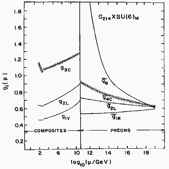
FIG. 1.: Unification of gauge couplings and their evolutions from $M_{Pl}=10^{19}$ Gev to $M_{Z}$ including threshold effects at lower and intermediate (metacolor) scales for the preonic gauge symmetry, $SU(2)_{L}\times U(1)_{R}\times SU(4)^{C}_{L+R}\times SU(6)_{M}$, with minimal two sets $\Delta_{L}$ and $\Delta_{R}$ fields and 10% mass difference between them.

B $G_{P}=SU(2)_{L}\times SU(2)_{R}\times U(1)_{B-L}\times SU(3)_{C}\times SU(6)_{M}$

In this case we, assume the gauge group to possess the left-right discrete symmetry starting from $\mu=\Lambda_{M}$ to $M_{Pl}$ with $\tilde{g}_{2L}(\mu)=\tilde{g}_{2R}(\mu)$. Denoting $i=1_{BL},2_{L},2_{R},3_{C}$ and 6 in (25), the one loop coefficients are,

$\displaystyle b^{\prime\prime}_{BL}=6,\ \ b^{\prime\prime}_{2L}=b^{\prime\prime}_{2R}=-6+{6\over 2}=-3$

$$b^{\prime\prime}_{3C}=-9+6=-3,\ \ b^{\prime\prime}_{6}=-3\times 6+6=-12$$ (33)

The equality of the coefficients $b^{\prime\prime}_{2L}=b^{\prime\prime}_{2R}=b^{\prime\prime}_{3C}$ signify unification of $SU(2)_{L}$ and $SU(3)_{C}$ gauge couplings from $\mu=\Lambda_{M}$ to $M_{Pl}$ at one-loop level when preons are in the fundamental representation and the metacolor symmetry is $SU(6)_{M}$. This is a common feature for $G_{fc}=G_{213}$, $G_{2113}$, and $G_{2213}$ when $G_{M}=SU(6)_{M}$ as can be seen in the following manner:

Suppose that $G=SU(N)_{M}$ for all the three types of $G_{fc}$. Then the one-loop coefficients for $SU(2)_{L}$ and $SU(3)_{C}$ are

$$b^{\prime\prime}_{2L}=-6+{N\over 2},\ \ b^{\prime\prime}_{3C}=-9+N$$ (34)

The one-loop unification for all values of $\mu$ starting from $\mu=\Lambda_{M}$ to $\mu=M_{U}$ is guarranted by the RGEs provided,

$$b^{\prime\prime}_{2L}=b^{\prime\prime}_{3C}=b^{\prime\prime}_{i}$$ (35)

with

$${1\over\tilde{\alpha}_{i}(\mu)}={1\over\tilde{\alpha}_{i}(M_{U})}+{b^{\prime\prime}_{i}\over 2\pi}\ln{M_{U}\over\mu},\ \ i=2L,3C$$ (36)

since $\tilde{\alpha}_{2L}(M_{U})=\tilde{\alpha}_{3C}(M_{U})$. But the equations (31) - (33) imply

$$N=6$$ (37)

proving that the metacolor gauge group is $SU(6)_{M}$ to achieve such one-loop unification from $\mu=\Lambda_{M}$ to $M_{U}$.

The matching conditions with $G_{fc}=G_{2213}$ at $\mu=\Lambda_{M}$ are

$\displaystyle\alpha^{-1}_{2}(\Lambda_{M})+\delta_{2}=\tilde{\alpha}^{-1}_{2L}(\Lambda_{M})=\tilde{\alpha}^{-1}_{2R}(\Lambda_{M})$

$\displaystyle\alpha^{-1}_{3}(\Lambda_{M})+\delta_{3}=\tilde{\alpha}^{-1}_{3}(\Lambda_{M})$

$$\alpha^{-1}_{1}(\Lambda_{M})+\delta_{1}={3\over 5}\tilde{\alpha}^{-1}_{2R}(\Lambda_{M})+{2\over 5}\tilde{\alpha}^{-1}_{BL}(\Lambda_{M})$$ (38)

Combining the first and the third eqs. in (35) and using (17) we have the following matching constraint ,

$$\tilde{\alpha}^{-1}_{BL}(\Lambda_{M})={5\over 2}\delta_{1}-{3\over 2}\delta_{2}+42.5$$ (39)

Approximate unification of gauge couplings at $M_{U}=10^{18}$ GeV with two sets of four fields is found to be possible when the $\Delta_{L}-\Delta_{R}$ mass difference is enhanced but remains within an acceptable limit corresponding to $\rho=M_{\Delta_{L}}/M_{\Delta_{R}}=1.6$. The individual masses and values of coupling constants at $\mu=M_{U}=10^{18}$ GeV and $\mu=\Lambda_{M}=10^{11}$ GeV are found to be,

$\displaystyle M_{\Delta_{L}}=7.8\times 10^{11}{\rm GeV},\ \ M_{\Delta_{R}}=4.7\times 10^{11}{\rm GeV}$

$$M_{\xi}=5.7\times 10^{11}{\rm GeV},\ \ M_{\sigma}=3.3\times 10^{12}{\rm GeV}$$ (41)

$\displaystyle\tilde{g}_{2L}(M_{U})=\tilde{g}_{2R}(M_{U})=0.640,\ \ \tilde{g}_{BL}(M_{U})=0.616$

$\displaystyle\tilde{g}_{3C}(M_{U})=0.643\pm 0.007,\ \ \tilde{g}_{6}(M_{U})=0.636$

$\displaystyle\tilde{g}_{2L}(\Lambda_{M})=\tilde{g}_{2R}(\Lambda_{M})=0.740,\ \ \tilde{g}_{BL}(\Lambda_{M})=0.508$

$$\tilde{g}_{3C}(\Lambda_{M})=0.745\pm 0.007$$ (42)

It is to be noted that the masses of $\Delta_{L}$ and $\Delta_{R}$ are constrained by spontaneous breaking of the left-right discrete symmetry and the $SU(2)_{R}\times U(1)_{B-L}$ gauge symmetry in $G_{2213}$, but there are no such constraints on the masses of $\xi$ and $\sigma$ fields. In no case the mass of any of the four fields should be widely different from $\Lambda_{M}$. From such considerations the mass $M_{\sigma}=33\Lambda_{M}$ in (37a) may be near the maximally permitted value. However, if there are more than two sets of degenerate $\sigma$-condensates in the model, its mass is likely to decrease. The evolution of gauge couplings from $M_{Z}$ to $M_{U}$ through $\Lambda_{M}$ is presented in Fig.2 where threshold effects at lower and intermediate scale are also exhibited.

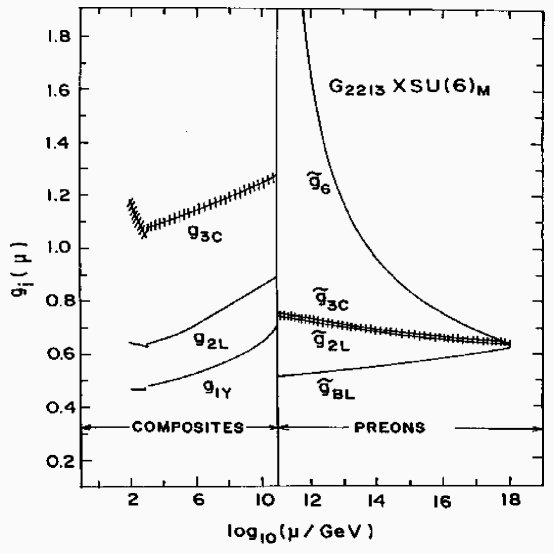
FIG. 2.: Same as Fig.1 but for the left-right symmetric preonic gauge group $SU(2)_{L}\times SU(2)_{R}\times U(1)_{B-L}\times SU(3)_{C}\times SU(6)_{M}$ with two sets of four fields, $\Delta_{L}$, $\Delta_{L}$, $\xi$ and $\sigma$, as described in the text and for 60% of mass difference between $\Delta_{L}$ and $\Delta_{R}$. The $SU(3)_{C}$ and the $SU(2)_{L}$ couplings follow almost the same trajectory from $\mu=10^{11}$ GeV to $10^{18}$ GeV because of one-loop unification in this range in the presence of $SU(6)_{M}$.

C $G_{P}=SU(2)_{L}\times U(1)_{Y}\times SU(3)_{C}\times SU(6)_{M}$

Corresponding to this symmetry $i=1Y,2L,3C$, and 6 in (25) and the one-loop coefficients are

$\displaystyle b^{\prime\prime}_{1Y}={7\times 6\over 10}={21\over 5},\ \ b^{\prime\prime}_{2L}=-3\times 2+{6\over 2}=-3$

$$b^{\prime\prime}_{3C}=-3\times 3+6=-3,\ \ b^{\prime\prime}_{6}=-3\times 6+6=-12$$ (43)

It is interesting to note that

$\displaystyle b^{\prime\prime}_{2L}=b^{\prime\prime}_{3C}=-3$

which implies unification of the preonic gauge couplings of $SU(2)_{L}$ and $SU(3)_{C}$ at one-loop level for all values of $\mu$ from $\Lambda_{M}$ to $M_{U}$ as explained in Sec V.B i.e.,

$\displaystyle\tilde{g}_{2L}(\mu)=\tilde{g}_{3C}(\mu),\ \ \mu=\Lambda_{M}\ \ {\rm to}\ \ M_{U}$

In order to achieve approximate unification of the gauge couplings at $M_{U}\simeq 10^{18}$ GeV, we need $\tilde{\alpha}^{-1}_{6}(M_{U})\simeq 27-30$. Neglecting threshold effects at $\Lambda_{M}$ gives

$\displaystyle\tilde{\alpha}^{-1}_{1Y}(\Lambda_{M})=\alpha^{-1}_{1}(\Lambda_{M})=26.7$

$\displaystyle\tilde{\alpha}^{-1}_{2L}(\Lambda_{M})=\alpha^{-1}_{2}(\Lambda_{M})=16.1$

$$\tilde{\alpha}^{-1}_{3C}(\Lambda_{M})=\alpha^{-1}_{3}(\Lambda_{M})=7.6\pm 0.6$$ (44)

Since

$${21\over 10\pi}\ln{M_{U}\over\Lambda_{M}}=10.8,\ \ {3\over 2\pi}\ln{M_{U}\over\Lambda_{M}}=7.7$$ (45)

eqs.(25) and (38)-(40) have the predictions,

$\displaystyle\tilde{\alpha}^{-1}_{1Y}(M_{U})=26.7-10.8=15.9$

$\displaystyle\tilde{\alpha}^{-1}_{2L}(M_{U})=16.1-7.7=23.8$

$$\tilde{\alpha}^{-1}_{3C}(M_{U})=7.6+7.7\pm 0.6=15.3\pm 0.6$$ (46)

Thus, starting from the CERN-LEP data at $\mu=M_{Z}$, including SUSY threshold effects, but ignoring the intermediate-scale-threshold corrections at $\mu=\Lambda_{M}$, there is no possibility of unification of gauge couplings at the preonic level with $G_{fc}=G_{213}$. When attempt is made to unify the gauge couplings including intermediate-scale threshold effects,we note from (41) that the corrections on each of $\alpha^{-1}_{1}(\Lambda_{M})$ and $\alpha^{-1}_{3}(\Lambda_{M})$ must be nearly two times as large as that on $\alpha^{-1}_{2}(\Lambda_{M})$. Including threshold effects,the matching conditions at $\Lambda_{M}$ are

$$\alpha_{i}^{-1}(\Lambda_{M})+\delta_{i}=\tilde{\alpha}^{-1}_{i}(\Lambda_{M}),\ \ i=1Y,2L,3C$$ (47)

We have observed that a good approximate unification of gauge couplings is possible with two sets of four fields if the $\Delta_{L}-\Delta_{R}$ mass difference is enhanced to correspond to the ratio $M_{\Delta_{R}}/M_{\Delta_{L}}=3.8$ for the following values of the individual masses,

$\displaystyle M_{\Delta_{L}}=1.3\times 10^{11}{\rm GeV},\ \ M_{\Delta_{R}}=5\times 10^{11}{\rm GeV}$

$$M_{\xi}=3.4\times 10^{11}{\rm GeV},\ \ M_{\sigma}=5.7\times 10^{11}{\rm GeV}$$ (48)

The values of the couplings at $M_{U}$ and $\Lambda_{M}$ are,

$\displaystyle\tilde{g}_{1Y}(M_{U})=0.633,\ \ \tilde{g}_{2L}(M_{U})=0.633,$

$\displaystyle\tilde{g}_{3C}(M_{U})=0.655\pm 0.007,\ \ \tilde{g}_{6}(M_{U})=0.633,$

$\displaystyle\tilde{g}_{1Y}(\Lambda_{M})=0.546,\ \ \tilde{g}_{2L}(\Lambda_{M})=0.735,$

$$\tilde{g}_{3C}(\Lambda_{M})=0.758\pm 0.007$$ (49)

The evolution of gauge couplings from $M_{Z}$ to $M_{U}$ are shown in Fig.3 where the approximate unification at $M_{U}$ and the one-loop unification of $\tilde{g}_{2L}(\mu)$ and $\tilde{g}_{3C}(\mu)$ for $\mu=\Lambda_{M}$ to $M_{U}$ are clearly exhibited. Nearly 70% difference between the $SU(3)_{C}$-gauge couplings of composites and preons compensated by threshold effects at $\Lambda_{M}$ is found to exist in this model. The corresponding differences between the $SU(2)_{L}$ and the $U(1)_{Y}$ gauge couplings are noted to be nearly 20% and 27%, respectively.

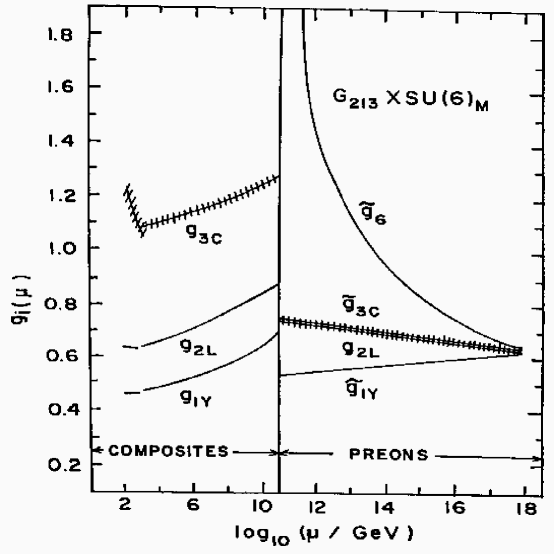
FIG. 3.: Same as Fig.2 but for the preonic gauge symmetry $SU(2)_{L}\times U(1)_{Y}\times SU(3)_{C}\times SU(6)_{M}$ and $M_{\Delta_{R}}/M_{\Delta_{L}}=3.8$ and two sets of four fields.

D $G_{P}=SU(2)_{L}\times U(1)_{R}\times U(1)_{B-L}\times SU(3)_{3C}\times SU(6)_{M}$

In this case $i=1R,BL,2L,3C$ and 6 and the one-loop coefficients are

$\displaystyle b^{\prime\prime}_{1R}={6\over 2}=3,\ \ b^{\prime\prime}_{BL}=6$

$\displaystyle b^{\prime\prime}_{2L}=-3\times 2+{6\over 2}=-3,\ \ b^{\prime\prime}_{3C}=-3\times 3+6=-3$

$$b^{\prime\prime}_{6}=-3\times 6+6=-12$$ (50)

As in the cases of $G_{fc}=G_{213}$ and $G_{2213}$, we find $b^{\prime\prime}_{2L}=b^{\prime\prime}_{3C}=-3$ in (45) signifying one-loop unification of preonic gauge couplings of $SU(2)_{L}$ and $SU(3)_{C}$ over the mass range $\mu=\Lambda_{M}$ to $M_{U}$. The matching conditions for gauge couplings at $\Lambda_{M}$ are

$${1\over\alpha_{1}(\Lambda_{M})}+\delta_{1}={3\over 5}{1\over\tilde{\alpha}_{1R}(\Lambda_{M})}+{2\over 5}{1\over\tilde{\alpha}_{BL}(\Lambda_{M})}$$ (52)

$${1\over\alpha_{2}(\Lambda_{M})}+\delta_{2}={1\over\tilde{\alpha}_{2L}(\Lambda_{M})}$$ (53)

$${1\over\alpha_{3}(\Lambda_{M})}+\delta_{3}={1\over\tilde{\alpha}_{3C}(\Lambda_{M})}$$ (54)

It is to be noted that one of the gauge couplings in the R.H.S of (46a), namely, $\tilde{\alpha}_{1R}(\Lambda_{M})$ or $\tilde{\alpha}_{BL}(\Lambda_{M})$, appear to remain undetermined. But in unified theories, once any of the coupling constant is known at $M_{U}$, the unification constraint gives other gauge couplings at that scale,

$\displaystyle\tilde{\alpha}_{2L}(M_{U})=\tilde{\alpha}_{1R}(M_{U})=\tilde{\alpha}_{BL}(M_{U})=\tilde{\alpha}_{3C}(M_{U})$

The knowledge of RGEs then determines the values of hitherto unknown couplings at lower scales, $\mu<M_{U}$, With two sets of four fields, we obtain $\delta_{1}=16.1$, $\delta_{2}=7.7$ and $\delta_{3}=15.1$ and all the four gauge couplings close to one another while satisfying approximate one loop unification, $g_{2}(\mu)=g_{3}(\mu)$, for all $\mu$ from $M_{U}$ to $\Lambda_{M}$. The masses of the four fields are,

$\displaystyle M_{\Delta_{L}}=10^{11}{\rm GeV},\ \ M_{\Delta_{R}}=4.4\times 10^{11}{\rm GeV}$

$$M_{\xi}=5\times 10^{11}{\rm GeV},\ \ M_{\sigma}=7.3\times 10^{11}{\rm GeV}$$ (56)

The gauge couplings at $M_{U}$ and $\Lambda_{M}$ are computed as

$\displaystyle\tilde{g}_{1R}(M_{U})=\tilde{g}_{BL}(M_{U})=0.630,\ \ \tilde{g}_{2L}(M_{U})=0.631$

$\displaystyle\tilde{g}_{3C}(M_{U})=0.642\pm 0.007,\ \ \tilde{g}_{6}(M_{U})=0.641$

$\displaystyle\tilde{g}_{1R}(\Lambda_{M})=0.563,\ \ \tilde{g}_{BL}(\Lambda_{M})=0.515$

$$\tilde{g}_{2L}(\Lambda_{M})=0.726,\ \ \tilde{g}_{3C}(\Lambda_{M})=0.743\pm 0.01$$ (57)

Apart from requiring $\rho^{-1}=M_{\Delta_{R}}/M_{\Delta_{L}}=4.4$, the model also needs about 70% threshold corrections for the $SU(3)_{C}$ coupling and nearly 20% for the $SU(2)_{L}$ coupling of composite fields that are introduced by these masses.

E $G_{P}=SU(2)_{L}\times SU(2)_{R}\times SU(4)_{L+R}^{C}\times SU(6)_{M}$

In this case the model possesses left-right discrete symmetry with $\tilde{g}_{2L}(\mu)=\tilde{g}_{2R}(\mu)$ for $\mu=\Lambda_{M}$ to $M_{U}$. The one loop coefficients are, $b^{\prime\prime}_{2L}=b^{\prime\prime}_{2R}=-3$, $b^{\prime\prime}_{4C}=-6$ and $b^{\prime\prime}_{6}=-12$. The coupling constants at $\Lambda_{M}$ are matched using

$\displaystyle\alpha^{-1}_{2}(\Lambda_{M})+\delta_{2}=\tilde{\alpha}^{-1}_{2L}(\Lambda_{M})=\tilde{\alpha}^{-1}_{2R}(\Lambda_{M})$

$\displaystyle\alpha^{-1}_{3}(\Lambda_{M})+\delta_{3}=\tilde{\alpha}^{-1}_{4C}(\Lambda_{M})$

$\displaystyle\alpha^{-1}_{1}(\Lambda_{M})+\delta_{1}={3\over 5}\tilde{\alpha}^{-1}_{2R}(\Lambda_{M})+{2\over 5}\tilde{\alpha}_{4C}^{-1}(\Lambda_{M})$

We have noted that it is impossible to achieve even a roughly approximate unification of gauge couplings with the above matching conditions unless the number of $\Delta_{L}$, $\Delta_{R}$, $\xi$ and $\sigma$ fields are unusually large and their masses are widely different from $\Lambda_{M}$. Thus the flavor-color symmetric gauge group $G_{fc}=G_{224}$ is unrealistic.

VI PROSPECTS OF SU(4)-METACOLOR

In this section, assuming the metacolor gauge symmetry to be $SU(4)_{M}$, we explore possible forms of flavor-color gauge symmetry $G_{fc}$ which could unify the relevant gauge couplings at $M_{U}$, or near the Planck scale. We follow strategies similar to those explained in Sec.V.

A $G_{P}=SU(2)_{L}\times U(1)_{R}\times U(1)_{B-L}\times SU(3)_{C}\times SU(4)_{M}$

With $G_{fc}=G_{2113}$ and $G_{M}=SU(4)_{M}$, the one loop coefficients in the RGEs of (25) are, $b^{\prime\prime}_{1R}=2$, $b^{\prime\prime}_{BL}=4$, $b^{\prime\prime}_{2L}=-4$, $b^{\prime\prime}_{3C}=-5$, $b^{\prime\prime}_{4}=-6$. The matching conditions at $\mu=\Lambda_{M}$ are given by (46a)-(46c). Although one of the gauge couplings, $\tilde{\alpha}_{1R}(\Lambda_{M})$ or $\tilde{\alpha}_{BL}(\Lambda_{M})$, is not determined by the matching conditions, this does not pose a problem in studying unification as explained in Sec.V.D. For the sake of simplicity we use $\tilde{\alpha}_{1R}(M_{U})=\tilde{\alpha}_{BL}(M_{U})$ at $M_{U}=10^{18}$ GeV. Unlike the case of $SU(6)_{M}$, where approximate unification was impossible under a small mass difference of 20% between $M_{\Delta_{L}}$ and $M_{\Delta_{R}}$, we find that with $SU(4)_{M}$, the gauge group achieves a good approximate unification with gaps between the gauge couplings closing in gradually as we approach $\mu=M_{Pl}$. The values of masses of the two sets of four fields, needed for approximate unification are

$\displaystyle M_{\Delta_{L}}=5.37\times 10^{10}{\rm GeV},\ \ M_{\Delta_{R}}=6.44\times 10^{10}{\rm GeV}$

$$M_{\sigma}=7.37\times 10^{11}{\rm GeV},\ \ M_{\xi}=10^{11}{\rm GeV}$$ (58)

where $M_{\Delta_{R}}/M_{\Delta_{L}}=1.2$. In Table VII we present values of the gauge couplings at three different mass scales $\mu=10^{11}$ GeV, $10^{18}$ GeV and $10^{19}$ GeV. The evolution of the gauge couplings of the effective gauge theories for preons, and quarks and leptons are presented in Fig.4 which exhibits a clear tandency of the preonic gauge couplings to converge near $\mu=M_{Pl}$. The remaining small differences among the couplings at $M_{Pl}$ are expected to be filled up by gravitational corrections. One remarkable feature of this model is that the difference between the $SU(3)_{C}$ couplings of composite fields and preons is negligible whereas that between the $SU(2)_{L}$ couplings is only 14%.

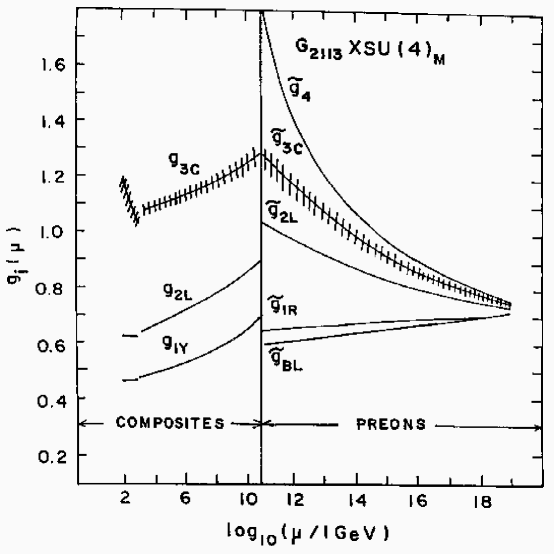
FIG. 4.: Same as Fig.1 but for the preonic gauge symmetry $SU(2)_{L}\times U(1)_{R}\times U(1)_{B-L}\times SU(3)_{C}\times SU(4)_{M}$ with two sets of three fields, $\Delta_{L}$, $\Delta_{R}$ and $\sigma$, and $M_{\Delta_{R}}/M_{\Delta_{L}}=1.2$.

B $G_{P}=SU(2)_{L}\times U(1)_{Y}\times SU(3)_{C}\times SU(4)_{M}$

In the notation of eq.(25), the one loop coefficients are $b^{\prime\prime}_{1Y}=14/5$, $b^{\prime\prime}_{2L}=-4$, $b^{\prime\prime}_{3C}=-5$, and $b^{\prime\prime}_{4}=-6$. The matching conditions are given by eq.(42). Restricting the difference between $M_{\Delta_{L}}$ and $M_{\Delta_{R}}$ to atmost 20% we find that approximate unification of gauge coupling at $\mu=10^{18}-10^{19}$ GeV is impossible. In Table VIII we present values of the gauge couplings $\mu=10^{19}$ GeV, $10^{18}$ GeV and $10^{11}$ GeV. Rather larger difference between the gauge couplings are found to be contradicting the idea of unification. However, we note that the coupling constants can unify at $M_{U}=10^{18}$ GeV only if the $\Delta_{L}-\Delta_{R}$ mass difference is allowed to be larger with $\rho^{-1}=M_{\Delta_{R}}/M_{\Delta_{L}}\cong 2.9$ corresponding to the following values of individual masses,

$\displaystyle M_{\Delta_{L}}=1.7\times 10^{10}{\rm GeV},\ \ M_{\Delta_{R}}=5.1\times 10^{10}{\rm GeV}$

$$M_{\xi}=1.96\times 10^{11}{\rm GeV},\ \ M_{\sigma}=7.37\times 10^{11}{\rm GeV}$$ (59)

Such a unification of gauge couplings and their evolution down to the $Z$-mass are presented in Fig.5. A very attractive feature of this model is that it needs almost negligible difference between $\tilde{g}_{3C}(\Lambda_{M})$ and $g_{3C}(\Lambda_{M})$ and also between $\tilde{g}_{1Y}(\Lambda_{M})$ and $g_{1Y}(\Lambda_{M})$.The model is found to require nearly 25% threshold correction on $SU(2)_{L}$ coupling of composites which is provided by the masses of two sets of four fields given in (49).

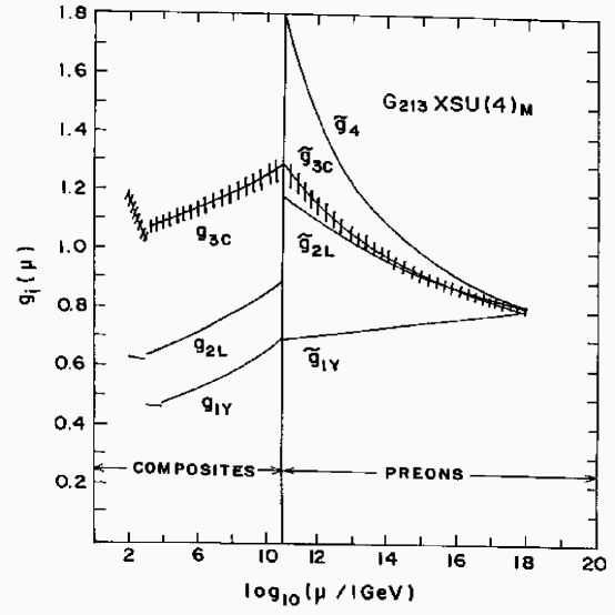
FIG. 5.: Same as Fig.3 but for the preonic gauge symmetry $SU(2)_{L}\times U(1)_{Y}\times SU(3)_{C}\times SU(4)_{M}$ and $M_{\Delta_{R}}/M_{\Delta_{L}}=2.9$.

C Difficulties with Other Flavor-Color Symmetries

The flavor-color groups investigated in VI.A-VI.B are the most successful ones in the presence of $SU(4)_{M}$. Difficulties faced with other symmetries are summarised as mentioned here. For $G_{P}=G_{214}\times SU(4)_{M}$, $b^{\prime\prime}_{2L}=-4$, $b^{\prime\prime}_{1R}=2$, $b^{\prime\prime}_{4C}=-8$ and $b^{\prime\prime}_{4}=-6$. Although the masses of two sets of all four fields needed for unification near $M_{Pl}$ are reasonable, with $M_{\Delta_{L}}/M_{\Delta_{R}}=1.2$, we find,

$\displaystyle\tilde{g}_{4C}(\mu)>\tilde{g}_{4}(\mu),\ \ \mu=10^{11}-10^{14}{\rm GeV}$

showing that $\tilde{g}_{4}(\mu)$ is no longer the highest coupling near $\mu=\Lambda_{M}$ responsible for binding the preons. This is against the basic assumption of the model. For $G_{P}=G_{2213}\times SU(4)_{M}$, $b^{\prime\prime}_{BL}=4$, $b^{\prime\prime}_{2L}=b^{\prime\prime}_{2R}=-4$, $b^{\prime\prime}_{3C}=-5$, and $b^{\prime\prime}_{4}=-6$. With two sets of four fields, the masses of $\Delta_{L}$ and $\Delta_{R}$ needed for approximate unification are nearly two orders lighter and those of $\xi$ and $\sigma$ one order heavier than $\Lambda_{M}$. For $G_{P}=G_{224}\times SU(4)_{M}$, either the number of some of the four types of fields are unusually large, or some of the masses are 5-6 orders different from $\Lambda_{M}$. Because of such undesirable features, $G_{fc}=G_{214}$, $G_{2213}$ or $G_{224}$ are unacceptable in the presence of $SU(4)_{M}$.

VII SUMMARY AND CONCLUSION

We have used the CERN-LEP measurements at $M_{Z}$ to study unity of forces and preonic gauge symmetries of the type $G_{P}=G_{fc}\times G_{M}$ in the scale-unifying preon model [12] which serves to provide a unified origin of the diverse mass scales and an explanation of family replication. Threshold effects form an important and essential part of gauge-coupling renormalization. Neglecting these effects has led to $G_{P}=G_{214}\times SU(5)_{M}$ as the only successful gauge symmetry of the preonic effective Lagrangian[15]. In this analysis, threshold effects are found to play a crucial role in determining the unification of forces near the Planck scale and, consequently, the gauge symmetry $G_{P}$ with new possibilities for $G_{fc}$ and $G_{M}=SU(6)_{M}$ or $SU(4)_{M}$.

With $SU(6)_{M}$ as metacolor gauge group, the most attractive possibility of flavor-color symmetry is found to be $G_{fc}=G_{214}$ for which a good approximate unification of gauge couplings occurs at $\mu=M_{Pl}=10^{19}$ GeV with only 10% to 20% mass difference between $\Delta_{L}(3,1,10^{C})$ and $\Delta_{R}(1,3,10^{*C})$ and the model needs just the minimal set of fields, $\Delta_{L}+\Delta_{R}$ and $\bar{\Delta}_{L}+\bar{\Delta}_{R}$, which are essential from considerations of left-right symmetry, preservation of SUSY down to the TeV scale, and spontaneous symmetry breaking of $G_{214}$ to the standard model gauge group at $\Lambda_{M}$.

For the next attractive possibility with $SU(6)_{M}$ corresponding to the left-right symmetric gauge group $G_{fc}=G_{2213}$, two sets of all the four fields, $\Delta_{L}$, $\Delta_{R}$, $\xi$ and $\sigma$, are needed and an approximate unification of gauge couplings is possible for acceptable value of the mass ratio, $\rho=M_{\Delta_{L}}/M_{\Delta_{R}}=1.6$, and $M_{\xi}=5.7\times 10^{11}$ GeV provided $M_{\sigma}=3.3\times 10^{12}$ GeV. Unification of gauge couplings is also observed with the standard model gauge group $G_{fc}=G_{213}$ and similar threshold effects with two sets of four fields provided the mass ratio $M_{\Delta_{R}}/M_{\Delta_{L}}=3.8$, and the individual masses of these fields are between $1.3\times 10^{11}$ GeV to $5.7\times 10^{11}$ GeV.

With $SU(4)_{M}$ as the metacolor gauge symmetry, two of the flavor-color gauge symmetries, $G_{213}$ and $G_{2113}$, appear to be quite successful in achieving good approximate unification of the relevant gauge couplings at $M_{U}=10^{18}$ GeV, and $10^{19}$ GeV, respectively. For $G_{fc}=G_{2113}$, the model needs the $\Delta_{L}-\Delta_{R}$ mass difference within 20% and two sets of three fields with reasonable values of masses near $\Lambda_{M}$. With the standard model gauge group $G_{fc}=G_{213}$ and $G_{M}=SU(4)_{M}$, the $\Delta_{L}-\Delta_{R}$ mass ratio needed is found to be such that $M_{\Delta_{R}}/M_{\Delta_{L}}=3$ and the other masses are $M_{\xi}=2\times 10^{11}$ GeV and $M_{\sigma}=7.4\times 10^{11}$ GeV. In this case two sets of all the four fields are needed.

All heavy and superheavy masses used in this paper for threshold effects refer to bare masses. They are devoid of wave function renormalisation effects which have been shown to be cancelled out by two-loop effects [20]. We assure that the bare masses are enough to produce threshold effects needed for new gauge symmetries. The cancellation observed in ref.[20] does not affect the results and conclusions of this analysis.

One of the most challenging problems is to derive the preonic model with one of the choices for the metacolor and flavor-color gauge symmetry, mentioned above, from a string theory. Also one of the major issues is to address some of the dynamical assumptions of the model as regards the preferred directions of symmetry breaking and the saturation of the composite spectrum, mentioned in the introduction [14,15]. In the absence of a derivation of the model from a deeper theory, apart from a number of unproven assumptions, the possible presence of more than one flavor-color symmetry groups above $\mu=\Lambda_{M}$ has an arbitrariness similar to SUSY $SO(10)$ with different possibilities for intermediate gauge symmetries. In spite of present theoretical limitations, the preonic approach seems promising because it is most economical and explains certain basic issues [12-15], by utilising primarily symmetries of the underlying theory and general results such as the Witten index theorem, rather than detailed dynamics. A crucial test of the model hinges on the detection of vectorial quarks and leptons with masses near 1-2 TeV. At present, there is no compelling evidence that quarks and leptons are composite as proposed in the model, although some possible signature has been investigated [16].

REFERENCES

• [1] J.C.Pati and A.Salam, Phys.Rev.D8, 1240 (1973); Phys.Rev.Lett.31, 661 (1973); Phys.Rev.D10, 275 (1974).
• [2] H.Georgi and S.L.Glssow, Phys.Rev.Lett.32, 438 (1974).
• [3] H.Georgi, in Particles and Fields, edited by C.E.Carlson (AIP, New York, 1975); H.Fritzsch and P.Minkowski, Ann.Phys. (N.Y.) 93, 193 (1975).
• [4] For a recent review see S.C.C.Ting, in Proceedings of the DPF 92 meeting, Fermilab, Batavia, Illinois, edited by C.Albright, P.H.Kasper, R.Raja and J.Yoh (World Scientific, Singapore, 1992) Vol.1, p53.
• [5] The LEP Collaborations ALEPH, DELPHI, L3 and OPAL and the LEP electroweak Working Group, CERN Report No.LEPEWWG/95-01; B.R.Webber, Proceedings of 27th International Conference on High Energy Physics, Glasgow, Scotland, 20-27 July(1994); J.Erler and P.Langacker, Phys.Rev.D52, 441 (1995); P.Langacker, Proceedings of the International Workshop on Supersymmetry and Fundamental Interactions (SUSY 1995), Palaiseau, France, 15-19 May(1995); P.Langacker and N.Polonsky, UPR-0642T, Report No.hep-ph/9503214.
• [6] S.Dimopoulos and H.Georgi, Nucl.Phys.B193, 150 (1991); N.Sakai, Z.Phys.C11, 153 (1982).
• [7] U.Amaldi, W.de Boer, and H.Furstenau, Phys.Lett.B260,447 (1991); U.Amaldi, W.de Boer, P.H.Frampton, H.Furstenau and J.T.Liu, Phys.Lett.B281, 374 (1992); J.Ellis, S.Kelly, and D.V.Nanopoulos, Phys.Lett.B260, 131 (1991); P.Langacker and N.Polonsky, Phys.Rev.D47, 4018(1993).
• [8] M.Green and J.Schwarz, Phys.Lett.B149, 117 (1984); D.Gross, J.Harvey, E.Martinec and R.Rohm, Phys.Rev.Lett.54, 502 (1985); P.Candelas, G.Horowitz, A.Strominger, and E.Witten, Nucl.Phys.B258, 46 (1985).
• [9] H.Kawai, D.Lewellen and S.Tye, Phys.Rev.Lett.57, 1832 (1986); I.Antoniadis, C.Bachas and C.Kounnas, Nucl.Phys.B289, 187 (1987); and J.Louis, Nucl.Phys.B444, 191 (1995); K.Dienes and A.Farazzi, Phys.Rev.Lett.75, 2646 (1995); Nucl.Phys.B457, 409 (1995).
• [10] V.S.Kaplunovsky, Nucl.Phys.B307, 145 (1988); V.S.Kaplunovsky and J.Louis, Nucl.Phys.B444, 191 (1995); K.Dienes and A.Farazzi, Phys.Rev.Lett.75, 2646 (1995); Nucl.Phys.B457, 409 (1995).
• [11] J.C.Pati, Phys.Lett.B144, 375 (1984); J.C.Pati, Proceedings of the Summer Workshop on β€œSuperstrings, Unified Theories and Cosmology, Trieste, Italy page 362-402(1987); J.C.Pati and H.Stremnitzer, Phys.Rev.Lett.56, 2152 (1986).
• [12] J.C.Pati, Phys.Lett.B228, 228 (1989).
• [13] K.S.Babu, J.C.Pati, and H.Stremnitzer, Phys.Lett.B256, 206 (1991).
• [14] K.S.Babu, J.C.Pati, and H.Stremnitzer, Phys.ReV.Lett.67, 1688 (1991).
• [15] K.S.Babu and J.C.Pati, Phys.Rev.D48, R1921 (1993).
• [16] K.S.Babu, J.C.Pati and X.Zhang, Phys.Rev.D46, 2190 (1992).
• [17] K.S.Babu, J.C.Pati and H.Stremnitzer, Phys.Lett.B256, 206 (1991); Phys.Lett.B264, 347 (1991).
• [18] E.Witten, Nucl.Phys.B185, 513 (1981).
• [19] J.C.Pati, M.Cvetic, and H.Sharatchandra, Phys.Rev.Lett.58, 851 (1987).
• [20] M.Shifman, Int.J.Mod.Phy.A11, 5761 (1996).
• [21] H.Georgi, H.Quinn, and S.Weinberg, Phys.Rev.Lett.33, 451 (1974).
• [22] S.Weinberg, Phy.Lett.B91, 51 (1980); L.Hall, Nucl.Phys.B178, 75 (1981).
• [23] P.Langacker and N.Polonsky, Phys.Rev.D47, 4028 (1993).
TABLE I.: Light and heavy spectrum in the scale-unifying preon model and their quantum numbers under $G_{224}$ and $G_{213}$.
Particle type and Particle type $G_{213}$-
$G_{214}$-quantum nos. under standard quantum nos.
model
L.H.quarks and leptons $(u,d)_{L}$, $(c,s)_{L}$, $(t,b)_{L}$ $(2,1/6,3)$
$q_{L}^{e,\mu,\tau}(2_{L},1,4^{*}_{C})$ $(\nu_{e},e)_{L}$, $(\nu_{\mu},\mu)_{L}$, $(\nu_{\tau},\tau)_{L}$ $(2,-1/2,1)$
R.H.quarks and leptons $u_{R}$, $c_{R}$, $t_{R}$ $(1,2/3,3)$
$q_{R}^{e,\mu,\tau}(1,2_{R},4^{*}_{C})$ $d_{R}$, $s_{R}$, $b_{R}$ $(1,-1/3,3)$
$e_{R}$, $\mu_{R}$, $\tau_{R}$ $(1,-1,1)$
$\nu_{e_{R}}$, $\nu_{\mu_{R}}$, $\nu_{\tau_{R}}$ $(1,0,1)$
L.H.vectorial quarks and $(U,D)_{L,R}$ $(2,1/6,3)$
leptons: $Q_{L,R}(2_{L},1,4^{*})$ $(N,E)_{L,R}$ $(2,-1/2,1)$
R.H.vectorial quarks and $(U^{\prime},D^{\prime})_{L,R}$ $(1,2/3,3)$
leptons $Q^{\prime}_{L,R}(1,2_{R},4^{*})$ $(N^{\prime},E^{\prime})_{L,R}$ $(1,-1/3,1)$
Bidoublet of Higgs $h_{u}$ $(2,1/2,1)$
scalars: $\phi(2,2,1)$ $h_{d}$ $(2,-1/2,1)$
Minimal sets of heavy Higgs
$\Delta_{L}^{1,2}(3,1,10^{C})$, $\Delta_{R}^{1,2}(1,3,10^{*C})$ see Table V see Table V
Other sets of heavy Higgs
$\xi^{1,2}(2,2,15)$, $\sigma^{1,2}(1,1,15)$ see Table IV see Table IV
TABLE II.: One-loop $\beta$-function coefficients for particles at lower threshold with their quantum numbers and assigned values of masses used for computation of threshold effects.
Particle type $G_{213}$- Mass $b_{1}^{\alpha}$ $b_{2}^{\alpha}$ $b_{3}^{\alpha}$
quantum nos. (GeV)
L.H. top $t_{L}$ $(2,1/6,3)$ 175 $1/30$ 1 $1/3$
R.H. top $t_{R}$ $(1,2/3,3)$ 175 $8/15$ 0 $1/3$
$u$-type Higgs $h_{u}$ $(2,1/2,1)$ 120 $1/10$ $1/6$ 0
$d$-type Higgs $h_{d}$ $(2,-1/2,1)$ 250 $1/10$ $1/6$ 0
L.H.vectorial quark
doublets $(U,D)_{L,R}$ $(2,1/6,3)$ 500 $2/15$ 2 $4/3$
R.H vectorial $u$-type
quarks $U^{\prime}_{L,R}$ $(1,2/3,3)$ 500 $16/15$ 0 $2/3$
R.H.vectorial $d$-type
quarks $D^{\prime}_{l,R}$ $(1,-1/3,3)$ 500 $4/15$ 0 $2/3$
L.H.vectorial lepton
doublets $(N,E)_{L,R}$ $(2,-1/2,1)$ 100 $2/5$ $2/3$ 0
R.H.vectorial charged
leptons $E^{\prime}_{L,R}$ $(1,-1,1)$ 100 $4/5$ 0 0
TABLE III.: Same as Table II but for superpartners only, and the number of squarks and sleptons correspond to summing over three flavors.
Particle type $G_{213}$- Mass $b_{1}^{\alpha}$ $b_{2}^{\alpha}$ $b_{3}^{\alpha}$
quantum nos. (GeV)
gluino (1, 0, 8) 150-200 0 0 23
wino (3, 0, 1) 100-150 0 $4/3$ 0
L.H.slepton doublets $(2,-1/2,1)$ 500-1500 $3/10$ $1/2$ 0
R.H.charged sleptons $(1,-1,1)$ 500-1500 $3/5$ 0
L.H.squark doublets $(2,1/6,3)$ 500-1500 $1/10$ $3/2$ 1
R.H.$u$-type squarks $(1,2/3,3)$ 500-1500 $4/15$ 0 $1/2$
R.H.$d$-type squarks $(1,1/3,3)$ 500-1500 $1/5$ 0 $1/2$
$u$-type Higgsino $(2,1/2,1)$ 100-300 $1/5$ $1/3$ 0
$d$-type Higgsino $(2,-1/2,1)$ 100-300 $1/5$ $1/3$ 0
TABLE IV.: One-loop $\beta$-function coefficients for the components of $G_{224}$-Higgs supermultiplet $\xi(2,2,15)$ near the metacolor scale under the standard gauge group $G_{213}$.
$G_{213}$ $b_{1}^{\alpha}$ $b_{2}^{\alpha}$ $b_{3}^{\alpha}$ $\sum b_{1}^{\alpha}$ $\sum b_{2}^{\alpha}$ $\sum b_{3}^{\alpha}$
submultiplet
$\xi_{1}(2,1/2,1)$ $3/10$ $1/2$ 0
$\xi_{2}(2,-1/2,1)$ $3/10$ $1/2$ 0
$\xi_{3}(2,-1/6,3)$ $1/10$ $3/2$ 1
$\xi_{4}(2,-7/6,3)$ $49/10$ $3/2$ 1
$\xi_{5}(2,-7/6,\overline{3})$ $49/10$ $3/2$ 1 $77/5$ 15 16
$\xi_{6}(2,1/6,\overline{3})$ $1/10$ $3/2$ 1
$\xi_{7}(2,1/2,8)$ $24/10$ 4 6
$\xi_{8}(2,-1/2,8)$ $24/10$ 4 6
TABLE V.: Same as Table IV but for $G_{224}$-multiplets, $\Delta_{L}(3,1,10^{C})$, $\Delta_{R}(1,3,10^{*C})$, and $\sigma(1,1,15)$.
$G_{213}$ $b_{1}^{\alpha}$ $b_{2}^{\alpha}$ $b_{3}^{\alpha}$ $\sum b_{1}^{\alpha}$ $\sum b_{2}^{\alpha}$ $\sum b_{3}^{\alpha}$
submultiplet
$\Delta_{R_{1}}(1,1,1)$ $3/5$ 0 0
$\Delta_{R_{2}}(1,2,1)$ $1/5$ 0 0
$\Delta_{R_{3}}(1,1/3,\overline{3})$ $1/5$ 0 $1/2$
$\Delta_{R_{4}}(1,2/3,\overline{3})$ $4/5$ 0 $1/2$
$\Delta_{R_{5}}(1,-4/3,\overline{3})$ $16/5$ 0 $1/2$ $78/5$ 0 9
$\Delta_{R_{6}}(1,1/3,\overline{6})$ $2/5$ 0 $5/2$
$\Delta_{R_{7}}(1,-2/3,\overline{6})$ $8/5$ 0 $5/2$
$\Delta_{R_{8}}(1,4/3,\overline{6})$ $32/5$ 0 $5/2$
$\Delta_{L_{1}}(3,1,1)$ $9/5$ 2 0
$\Delta_{L_{2}}(3,1/3,\overline{3})$ $3/5$ 6 $3/2$ $18/5$ 20 9
$\Delta_{L_{3}}(3,-1/3,6)$ $6/5$ 12 $15/2$
$\sigma_{1}(1,-2/3,3)$ $4/5$ 0 $1/2$
$\sigma_{2}(1,2/3,3)$ $4/5$ 0 $1/2$ $8/5$ 0 4
$\sigma_{3}(1,0,8)$ 0 0 3
TABLE VI.: Gauge couplings at different mass scales in the presece of two sets of relevant Higgs superfields for the preonic symmetry $G_{P}=SU(2)_{L}\times U(1)_{R}\times SU(4)_{L+R}^{C}\times SU(6)_{M}$, with $M_{\Delta_{L}}=3.5\times 10^{11}$ GeV and $\rho=M_{\Delta_{L}}/M_{\Delta_{R}}=1.1$. Note that the four gauge couplings converge within 4% as $\mu$ approaches $10^{19}$ GeV.
Mass scale ($\mu$) $\tilde{g}_{1R}(\mu)$ $\tilde{g}_{2L}(\mu)$ $\tilde{g}_{4C}(\mu)$ $\tilde{g}_{6}(\mu)$
(GeV)
$10^{19}$ 0.580 0.617 $0.624\pm 0.007$ 0.613
$10^{18}$ 0.570 0.628 $0.646\pm 0.007$ 0.658
$10^{11}$ 0.527 0.722 $0.927\pm 0.007$ β€”
TABLE VII.: Values of gauge couplings at different mass scales obtained using two sets of relevant Higgs superfields for the preonic gauge symmetry $G_{P}=SU(2)_{L}\times U(1)_{I_{3R}}\times U(1)_{B-L}\times SU(3)_{C}\times SU(4)_{M}$ with $M_{\Delta_{L}}=5.3\times 10^{10}$ GeV, $M_{\Delta_{R}}=6.4\times 10^{10}$ GeV, $M_{\sigma}=7.3\times 10^{11}$ GeV and $\rho^{-1}=M_{\Delta_{R}}/M_{\Delta_{L}}=1.2$.
Mass scale ($\mu$) $\tilde{g}_{2L}(\mu)$ $\tilde{g}_{3C}(\mu)$ $\tilde{g}_{1R}(\mu)$ $\tilde{g}_{BL}(\mu)$ $\tilde{g}_{4}(\mu)$
(GeV)
$10^{19}$ 0.731 $0.753\pm 0.013$ 0.720 0.732 0.764
$10^{18}$ 0.755 $0.792\pm 0.013$ 0.710 0.710 0.806
$10^{11}$ 1.034 $1.32\pm 0.05$ 0.647 0.598 1.80
TABLE VIII.: Gauge couplings at different mass scales but for $G_{P}=SU(2)_{L}\times U(1)_{Y}\times SU(3)_{C}\times SU(4)_{M}$. Here $M_{\sigma}=7.3\times 10^{11}$ GeV throughout. For the case(a) $M_{\Delta_{L}}=1.3\times 10^{10}$ GeV, $M_{\Delta_{R}}=1.6\times 10^{10}$ GeV, $M_{\Delta_{R}}/M_{\Delta_{L}}=1.2$, and $M_{\xi}=4\times 10^{11}$ GeV, but $M_{\Delta_{L}}=1.7\times 10^{10}$ GeV, $M_{\Delta_{R}}=5.1\times 10^{10}$ GeV, $M_{\Delta_{R}}/M_{\Delta_{L}}=2.9$, and $M_{\xi}=1.96\times 10^{11}$ GeV for the case (b).
Mass scale ($\mu$) $\tilde{g}_{1}(\mu)$ $\tilde{g}_{2L}(\mu)$ $\tilde{g}_{3C}(\mu)$ $\tilde{g}_{4}(\mu)$
(GeV)
(a) $10^{18}$ $0.872\pm 0.005$ $0.798\pm 0.008$ $0.808\pm 0.06$ 0.859
$10^{11}$ $0.707\pm 0.004$ $1.149\pm 0.01$ $1.4\pm 0.07$ 2.5
(b) $10^{18}$ $0.802\pm 0.004$ $0.806\pm 0.007$ $0.784\pm 0.015$ 0.806
$10^{11}$ $0.686\pm 0.002$ $1.175\pm 0.01$ $1.287\pm 0.015$ 1.80