bla $\scriptstyle{\rm UMHEP-453}$

The leading chiral electromagnetic correction to the nonleptonic $\Delta I=3/2$ amplitude in kaon decays

Vincenzo Cirigliano^a, John F. Donoghue^b and Eugene Golowich^b

^a Dipartimento di Fisica dell’Università and I.N.F.N.

Via Buonarroti,2 56100 Pisa (Italy)

vincenzo@het.phast.umass.edu

^b Department of Physics and Astronomy

University of Massachusetts

Amherst MA 01003 USA

donoghue@het.phast.umass.edu

gene@het.phast.umass.edu

In kaon decay, electromagnetic radiative corrections can generate shifts in the apparent $\Delta I=3/2$ amplitude of order $\alpha A_{0}/A_{2}\sim 22\alpha$. In order to know the true $\Delta I=3/2$ amplitude for comparison with lattice calculations and phenomenology, one needs to subtract off this electromagnetic effect. We provide a careful estimate of the leading electromagnetic shift in the chiral expansion of the amplitude, which shows that it is smaller than naive expectations, with a fractional shift of $\delta A_{2}^{\rm(em)}/A_{2}=-0.016\pm 0.01$.

1 Introduction

The $\Delta I=1/2$ enhancement of nonleptonic kaon decays is a well-known feature which has still not been completely explained. Most existing lattice calculations find a $\Delta I=3/2$ amplitude which is a factor of two larger than the experimental value. This $\Delta I=3/2$ amplitude also enters present phenomenology through the chiral determination of the $B_{K}$ parameter which is part of the Standard Model prediction of CP violation. The chiral calculation [2] (which relates $B_{K}$ to the experimental $\Delta I=3/2$ amplitude) disagrees with the quenched lattice calculation for $B_{K}$ also by about a factor of two. At present we do not know if the disagreement in $B_{K}$ is due to the failure of the lattice approach to reproduce the experimental amplitude or if there are large chiral corrections responsible for the difference.

In both these applications, we need to know the true $\Delta I=3/2$ effect. Since the $\Delta I=1/2$ amplitude is so much larger, it is possible that electromagnetic corrections to it may simulate an effect which is similar to the small $\Delta I=3/2$ amplitude. These electromagnetic corrections enter at order $\alpha A_{0}=A_{0}/137$, which can be comparable to a sizeable portion of the $\Delta I=3/2$ amplitude $A_{2}\simeq A_{0}/22$. The possibility then emerges that the relevant experimental amplitude (without electromagnetism) could differ significantly from that presently being used in phenomenology.

Although the literature on this subject extends over many years, e.g. see Refs. [3, 4, 5, 6], the issue has not yet received a definitive treatment. It is our aim in this paper to provide an analysis using the most up-to-date tools which will yield a reliable estimate of this effect. In a longer paper, we will present a more comprehensive analysis of electromagnetic radiative corrections in kaon decays. The full system, particularly the decay $K_{S}\to\pi^{+}\pi^{-}$, brings in several additional complications, such as the Coulomb effect on the final state, the violations of Watson’s theorem from the mixing of final states and the induced $\Delta I=5/2$ effect. However, the decay $K^{+}\to\pi^{+}\pi^{0}$ is particularly simple and can by itself be used to answer the question that we have raised above. Among our results in this paper are:

1. The long distance portion of the leading chiral result satisfies the relation ${\cal M}_{\rm LD}=-2g_{8}(\delta m_{\pi}^{2})_{\rm LD}/F_{\pi}^{2}$ where $(\delta m_{\pi}^{2})_{\rm LD}$ is the long distance part of the pion electromagnetic mass difference and the other constants are defined below.

2. This leading long distance effect is canceled exactly by the effect of pion mass differences in the usual weak amplitude.

3. There are, however, residual effects coming from intermediate energies and the electroweak penguin operator. Although we allow generous uncertainties associated with intermediate energies, it is clear that the net residual effect is quite small.

2 Chiral Analysis

Chiral symmetry provides the framework for structuring our calculation. We first replace the calculation of the decay amplitude $A_{+0}(p_{K},p_{\pi^{+}},p_{\pi^{0}})$ with the simpler $K^{+}$-to-$\pi^{+}$ matrix element by taking the soft pion limit,

$$A_{+0}(p,p,0)=-{i\over 2F_{\pi}}{\cal M}(p)\ \ ,$$ (1)

where

$${}_{\rm out}\langle\pi^{+}(p^{\prime})|K^{+}(p)\rangle_{\rm in}=i(2\pi)^{4}\delta^{(4)}(p^{\prime}-p)\ \ {\cal M}(p)\ \ .$$ (2)

For most of our analysis, we shall work with the leading chiral component ${\cal M}(0)$

$${\cal M}(p)\ =\ {\cal M}(0)\ +\ {\cal O}(p^{2})+\dots\ \ ,$$ (3)

and add in (small) ${\cal O}(p^{2})$ contributions at the end.

Figure 1: Combined weak-electromagnetic transitions of quarks.

2.1 The Chiral and Electromagnetic-penguin Components

At the quark level, electromagnetic corrections to the weak transition ${\bar{s}}+u\to{\bar{d}}+u$ fall into two distinct classes (cf Fig. 1), which we call the chiral (CH) and electromagnetic-penguin (EMP) components,

$${\cal M}(0)={\cal M}_{\rm CH}+{\cal M}_{\rm EMP}\ \ .$$ (4)

The amplitude ${\cal M}_{\rm CH}$ is associated with the long-range and intermediate-range contributions of the process in Fig. 1(a) (along with all other diagrams in which a photon is exchanged between the quark legs). We note that the short distance part of such transitions leads merely to an overall shift in the strength of the nonleptonic interaction. Using the procedure described in Ref. [7], this is equivalent to an effective Fermi constant defined as

$$G_{NL}({\bar{\mu}})=G_{\mu}\left[1+{2\alpha\over 3\pi}\ln\left({M_{W}\over{\bar{\mu}}}\right)\right]\ \ ,$$ (5)

where ${\bar{\mu}}$ is an energy scale lying in the region where perturbation theory is valid and $G_{\mu}$ is the Fermi constant measured in muon decay. This shift does not lead to mixing of isospin amplitudes and is irrelevant for the purposes of this paper. Calculation of the long and intermediate range contributions to ${\cal M}_{\rm CH}$ is carried out in Sect. 3.1 and Sect. 3.2.

The amplitude ${\cal M}_{\rm EMP}$ corresponding to the electromagnetic penguin operator of Fig. 1(b) will have both long-distance and short-distance components. These are described in Sect. 3.3. Determination of the full amplitude ${\cal M}$ is carried out in Sect. 3.4, with special attention paid to the relative phase between ${\cal M}_{\rm CH}$ and ${\cal M}_{\rm EMP}$ and to the matching of long and short distances.

2.2 Chiral Lagrangians

We now introduce some useful chiral lagrangians. The weak interactions involve left-handed currents only and the nonleptonic hamiltonian has an octet and 27-plet component. The lowest-order weak lagrangian for the dominant octet portion involves two derivatives,

$${\cal L}_{8}\ =\ g_{8}\,{\rm Tr}\,\left(\lambda_{6}D_{\mu}UD^{\mu}U^{\dagger}\right)\ \ ,$$ (6)

with $|g_{8}|\simeq 7.8\cdot 10^{-8}~{}F_{\pi}^{2}$.

Electromagnetic corrections involve both left-handed and right-handed effects, and can lead to lagrangians which do not involve derivatives. For example, one of the effects of electromagnetism is to shift the charged pion masses, an effect described at lowest order by the lagrangian

$${\cal L}_{\rm ems}=g_{\rm ems}\,{\rm Tr}\,\left(QUQU^{\dagger}\right)\ \ .$$ (7)

The parameter $g_{\rm ems}$ is fixed from the pion electromagnetic mass splitting,

$$\delta m_{\pi}^{2}\ =\ {2\over F_{\pi}^{2}}g_{\rm ems}\ \ .$$ (8)

There is also the lagrangian which describes the leading electromagnetic correction to the weak interactions to leading chiral order,

$${\cal L}_{\rm emw}=g_{\rm emw}\,{\rm Tr}\,\left(\lambda_{6}UQU^{\dagger}\right)\ \ ,$$ (9)

where $g_{\rm emw}$ is an a priori unknown coupling constant. Knowledge of $g_{\rm emw}$ is equivalent to that of the matrix element ${\cal M}(0)$ as the two are related in the chiral limit by

$${\cal M}(0)\ =\ {2\over F_{\pi}^{2}}~{}g_{\rm emw}\ \ .$$ (10)

In Sect. 3, we present a detailed calculation of ${\cal M}(0)$ (and thus of $g_{\rm emw}$) and as a consequence reveal an approximate numerical relationship between $g_{\rm emw}$ and $g_{\rm ems}$. Then in Sect. 4, we turn to the full $A_{+0}$ amplitude, including also the effects that arise at the next chiral order (${\cal O}(p^{2})$) from the photon loop calculation.

3 Calculation of the leading chiral amplitude

To fully calculate the relevant amplitude, we need to consider contributions from all scales. We will recognize three regions of the virtual photon momentum:

1. very low energies $Q^{2}<\Lambda^{2}$ with $\Lambda\sim m_{\rho}$,

2. high energies with $Q^{2}>\mu^{2}$   ($\mu\sim 1.5\to 2.5~{}{\rm GeV}$),

3. intermediate energies between these two regions.

In the lowest energy regime, we may use chiral techniques to obtain the leading effect. At high energies, the short distance analysis of QCD will be employed. The most important ingredient of the treatment of intermediate energies is the requirement of matching these two regions. This will be modelled on physics which is reliably known in the case of electromagnetic mass shifts.

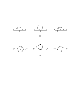
Figure 2: Electromagnetic corrections to the $K^{+}$-to-$\pi^{+}$ transition.

3.1 Long Distance Component of ${\cal M}_{\rm CH}$

The very long distance component can be calculated from the combined chiral lagrangian of the strong weak and electromagnetic interactions in the chiral limit. In the diagrams of Fig. 2(a), one finds after Wick rotation a matrix element

$${\cal M}_{\rm LD}\ =\ -{3\alpha g_{8}\over 2\pi F_{\pi}^{2}}\int_{0}^{\Lambda^{2}}dQ^{2}\ \ ,$$ (11)

where $\Lambda$ represents the upper end of the low-energy region. We note that a similar calculation of the electromagnetic mass shift of the charged pion, Fig. 3(a), yields

$$\delta m_{\pi}^{2}\Big{|}_{\rm LD}\ =\ {3\alpha\over 4\pi}\int_{0}^{\Lambda^{2}}dQ^{2}\ \ ,$$ (12)

The similarity of the two can be motivated by the fact that in the former calculation the weak vertex in the loop introduces a factor of $l^{2}$ ($l$ is the loop momentum) which compensates one of the two propagators, yielding an effect similar to that of Fig. 3(a). At this stage, it is a curiosity to note that the choice of $\Lambda^{2}=m_{\rho}^{2}$ provides an accurate description of the pion mass difference. However, we will see below that this is not an accident — that reliably known physics cuts off the integral above the rho mass. For our purposes at this stage, this similarity is the first indication of the relation

$${\cal M}_{\rm LD}=-2{g_{8}\over F_{\pi}^{2}}(\delta m_{\pi}^{2})_{\rm LD}$$ (13)

or $(g_{\rm emw})_{\rm LD}=-g_{8}{\delta m_{\pi}^{2}}_{\rm LD}$. This could be derived somewhat more formally by using a rotation to the basis where the kinetic energy matrix is diagonalized. [9] The application of long distance electromagnetic mass shifts to the rotated basis is equivalent to the above relation in the non-rotated basis.

Figure 3: Pion electromagnetic mass shift.

3.2 Intermediate Energy Component of ${\cal M}_{\rm CH}$

A prototype for dealing with the intermediate energies is the pion electromagnetic mass difference. The accumulated wisdom of many studies has given us an accurate guide to the physics of this process. A rigorous approach would involve the sum rule of Das et al [10], in which $\delta m_{\pi}^{2}$ is expressed in terms of the difference of the experimental vector and axialvector spectral functions $(\rho_{V}-\rho_{A})(s)$. This has been analysed successfully using experimental data and QCD constraints. [11] A simplified expression that captures the essential physics is obtained upon saturating $\rho_{V}$ and $\rho_{A}$ respectively with the vector $\rho$ resonance and the axialvector resonance $a_{1}$. This yields

$$\delta m_{\pi}^{2}\ = \ {3\alpha\over 4\pi}\int_{0}^{\infty}dQ^{2}\left[1-{F_{V}^{2}\over F_{\pi}^{2}}{Q^{2}\over Q^{2}+m_{\rho}^{2}}+{F_{A}^{2}\over F_{\pi}^{2}}{Q^{2}\over Q^{2}+m_{a_{1}}^{2}}\right]$$ (14)

$$= {3\alpha\over 4\pi}\int_{0}^{\infty}dQ^{2}\ {m_{a_{1}}^{2}\over Q^{2}+m_{a_{1}}^{2}}\cdot{m_{\rho}^{2}\over Q^{2}+m_{\rho}^{2}}\ \ .$$

The second form is found when the resonance couplings and masses satisfy the Weinberg sum rules, which are required in order to obtain the right high energy behavior. The long-distance amplitude given in Eq. (12) has been softened at values of $Q^{2}$ above the meson masses so that $m_{\rho}$ and $m_{a_{1}}$ act as the effective cutoff for the integral. This result is equally well reproduced by introducing resonance couplings to the effective lagrangian and imposing the Weinberg sum rules on the masses and couplings. This involves the diagrams of Fig. 3(b).

What is the analogous statement for ${\cal M}_{\rm CH}\equiv{\cal M}_{\rm LD}+{\cal M}_{\rm INT}+{\cal M}_{\rm SD}$? First, we recall from the discussion surrounding Eq. (5) that, rather than contributing to the isospin mixing effect, the dominant effect of the short distance (SD) component is to renormalize the Fermi constant. The full chiral amplitude thus experiences important contributions only from long and intermediate distance effects and must vanish in the short distance region. Combining results from the previous sections, our form for the long and intermediate distance regions is

$${\cal M}_{\rm CH}=-{3\alpha g_{8}\over 2\pi F_{\pi}^{2}}\int_{0}^{\mu^{2}}dQ^{2}\left[1-{B_{V}Q^{2}\over Q^{2}+m_{V}^{2}}-{B_{A}Q^{2}\over Q^{2}+m_{A}^{2}}+{Cm_{A}^{2}Q^{2}\over(Q^{2}+m_{A}^{2})^{2}}\right]\ \ ,$$ (15)

where the $Q^{2}$-integral for ${\cal M}_{\rm CH}$ is seen to be effectively cut off at some scale $\mu^{2}$. The quantities $B_{V}$, $B_{A}$ and $C$ in the above contain couplings from the weak interaction resonance lagrangians. [12] It is of course possible to model these couplings, and we have done so. However, it is more to the point to implement the constraint (discussed earlier) that ${\cal M}_{\rm CH}$ receive no mixing contribution from the high-$Q^{2}$ region. Thus these constants must be constrained such that the ampliude vanish at the matching to the short distance region. For this to occur, we require that the large $Q^{2}$ limit of the integrand ($Q^{2}\gg m_{V,A}^{2}$) approach zero rather than a constant, i.e.

$$B_{V}\ +\ B_{A}\ =\ 1\ \ .$$ (16)

We further constrain this amplidude by choosing the matching scale $Q=\mu$ at which the amplitude vanish. If $m_{V}$ and $m_{A}$ were equal this constraint would determine unknown $C$ in the integrand of Eq. (15). In our numerical study, we choose $\mu$ to lie between $1.5$ GeV and $2.5$ GeV and treat the resulting variation as one of the uncertainties of the calculation. Of course, the difference between $m_{V}$ and $m_{A}$ leads to a slight further uncertainty. To model this effect, we have explored models for the resonance couplings [13] —which weight the axialvector and vector resonances differently. It is found that this uncertainty is smaller than that associated with variation of the matching scale $\mu$.

3.3 Determination of ${\cal M}_{\rm EMP}$

As we shall show in the following, the electromagnetic penguin (EMP) operator of Fig. 1(b) gives rise to contributions over all distance scales. It is, however, the sole source of meaningful short distance effects in our calculation of electromagnetic corrections to $A_{2}$. If the numerically tiny $t$-quark contribution is omitted, the EMP hamiltonian takes the form,

$$-i{\cal H}_{\rm EMP}={\bar{G}}\int{d^{4}q\over(2\pi)^{4}}{I^{\mu\nu}(q,{\bar{\mu}})\over q^{2}+i\epsilon}$$

$$\phantom{xxx}\times\int d^{4}y\ e^{-iq\cdot y}~{}T\left[{\bar{s}}(0)\gamma_{\mu}(1+\gamma_{5})d(0){\bar{q}}(y)Q\gamma_{\nu}q(y)\right]\ \ ,$$ (17)

where $q=u,d,s$ is a light-quark field, ${\bar{G}}\equiv 2e^{2}G_{F}V_{us}^{*}V_{ud}/(3\sqrt{2})$, and $I^{\mu\nu}(q,{\bar{\mu}})$ represents the effect of the quark-antiquark loop in the EMP operator. In evaluating $I^{\mu\nu}(q,{\bar{\mu}})$, it is understood that at the lower end, the loop momentum is cut off at scale ${\bar{\mu}}$ (cf see Eq. (21)). The dependence on ${\bar{\mu}}$ is logarithmic and thus quite weak.

Figure 4: Electromagnetic penguin and the $K^{+}$-to-$\pi^{+}$ transition.

It can be shown [14] that in the chiral limit the $K^{+}$-to-$\pi^{+}$ matrix element of ${\cal H}_{\rm EMP}$ (cf Fig. 4) is expressible as

$$\lim_{p=0}~{}\langle\pi^{+}(p)|T\left[{\bar{s}}(0)\gamma_{\mu}(1+\gamma_{5})d(0){\bar{q}}(y)Q\gamma_{\nu}q(y)\right]|K^{+}(p)\rangle$$

$$\phantom{xxxx}=-i{2\over F_{\pi}^{2}}\int{d^{4}k\over(2\pi)^{4}}\ e^{ik\cdot y}\left(k_{\mu}k_{\nu}-k^{2}g_{\mu\nu}\right)\left[\Pi_{\rm V3}-\Pi_{\rm A3}\right](k^{2})\ \ ,$$ (18)

where $\Pi_{\rm V3}$, $\Pi_{\rm A3}$ are the isospin vector and axialvector correlators. In the chiral limit, the $K^{+}$-to-$\pi^{+}$ matrix element of the EMP operator thus becomes

$$\lim_{p=0}~{}\langle\pi^{+}(p)|{\cal H}_{\rm EMP}|K^{+}(p)\rangle$$

$$\phantom{xxx}={2{\bar{G}}\over F_{\pi}^{2}}\int{d^{4}q\over(2\pi)^{4}}{I^{\mu\nu}(q,{\bar{\mu}})\over q^{2}+i\epsilon}\left(q_{\mu}q_{\nu}-q^{2}g_{\mu\nu}\right)\left[\Pi_{\rm V3}-\Pi_{\rm A3}\right](q^{2})\ \ .$$ (19)

This expression describes the EMP effect over all scales of the virtual photon (euclidean) momentum,

$${\cal M}_{\rm EMP}=-{3{\bar{G}}M_{V}^{2}M_{A}^{2}\over(2\pi)^{4}}\int_{0}^{\infty}dQ^{2}\ {Q^{2}\over(Q^{2}+M_{V}^{2})(Q^{2}+M_{A}^{2})}I(Q^{2},{\bar{\mu}}^{2})\ \ ,$$ (20)

where we have expressed the $Q^{2}$ dependence of the correlators in terms of vector and axialvector pole terms, an approximation we know to be valid to within a few per cent. An explicit form for the EMP integral $I(Q^{2},{\bar{\mu}}^{2})$ is

$$I(Q^{2},{\bar{\mu}}^{2}) = \int_{0}^{1}dx\ x(1-x)~{}\bigg{[}\ln{{\bar{\mu}}^{2}+m_{c}^{2}+Q^{2}x(1-x)\over{\bar{\mu}}^{2}+m_{u}^{2}+Q^{2}x(1-x)}$$ (21)

$$+{m_{c}^{2}+Q^{2}x(1-x)\over{\bar{\mu}}^{2}+m_{c}^{2}+Q^{2}x(1-x)}-{m_{u}^{2}+Q^{2}x(1-x)\over{\bar{\mu}}^{2}+m_{u}^{2}+Q^{2}x(1-x)}\bigg{]}\ \ .$$

where $m_{c}$ and $m_{u}$ are the $c$-quark and $u$-quark masses. The latter vanishes in the chiral limit.

3.4 Matching

The final step in determining ${\cal M}(0)$ is to add together the components ${\cal M}_{\rm CH}$ and ${\cal M}_{\rm EMP}$. This is displayed schematically in Fig. 5 which depicts the integrands in the $Q^{2}$ integrals and indicates that the short-distance contribution is numerically much smaller than the long-distance contribution.

Figure 5: Schematic of matching.

It would appear that the calculation must contain an ambiguity arising from ignorance of the relative phase between ${\cal M}_{\rm CH}$ and ${\cal M}_{\rm EMP}$ or equivalentally of the sign of $g_{8}$. However, we can infer that $g_{8}<0$ from the following argument. From the $\Delta I=1/2$ chiral lagrangian of Eq. (6), we have for the $K^{0}\to(2\pi)_{I=0}$ amplitude,

$$A_{0}=i{\sqrt{2}\over F_{\pi}^{3}}\left(m_{K}^{2}-m_{\pi}^{2}\right)~{}g_{8}\ \ .$$ (22)

Alternatively, we can obtain $A_{0}$ using the effective lagrangian of the Standard Model

$${\cal L}_{\Delta S=1}=-{G_{F}\over\sqrt{2}}V_{ud}V_{us}^{*}\sum_{i}\ c_{i}(\mu){\cal O}_{i}\ \ ,$$ (23)

together with the vacuum saturation approximation (VSA),

$$\langle(2\pi)_{I=0}|{\cal O}_{i}|K^{0}\rangle=B_{i}^{(0)}\langle(2\pi)_{I=0}|{\cal O}_{i}|K^{0}\rangle_{\rm VSA}\ \ ,$$ (24)

to write

$$A_{0}=-iG_{F}F_{\pi}V_{ud}V_{us}^{*}\left(m_{K}^{2}-m_{\pi}^{2}\right)~{}g_{8}^{\rm eff}\ \ ,$$ (25)

with

$$g_{8}^{\rm eff}=\sqrt{3\over 2}\bigg{[}-{1\over 6}c_{1}B_{1}^{(0)}+{5\over 9}c_{2}B_{2}^{(0)}+{1\over 3}c_{3}B_{3}+c_{4}B_{4}$$

$$\phantom{xxxxx}-16\left({\langle{\bar{q}}q\rangle\over F_{\pi}^{3}}\right)^{2}L_{5}\left({1\over 3}c_{5}B_{5}+c_{6}B_{6}\right)\bigg{]}\ \ .$$ (26)

In the above, $L_{5}$ is a coefficient in the Gasser-Leutwyler ${\cal O}(p^{4})$ chiral lagrangian, the superscripts on $B_{1}^{(0)}$, $B_{2}^{(0)}$ signify $I=0$ for the final state $2\pi$ pair, and we refer the reader to Ref. [15] for further details. Since (with the exception of $B_{3}$) the $\{B_{i}\}$ are all positive, the $\{|c_{i}|\}$ have been determined at NLO and specifically $c_{1},c_{6}<0$, we conclude with reasonable certainty that $g_{8}<0$.

The analysis described throughout this section then leads to the following value, expressed in units of $g_{8}\delta m_{\pi}^{2}$, for the coupling $g_{\rm ewp}$ of Eq. (9),

$${g_{\rm emw}\over g_{8}\delta m_{\pi}^{2}}\ =\ -0.62\pm 0.19\ \ .$$ (27)

The uncertainty arises almost entirely from variation of the parameter $\mu$ (we have set ${\bar{\mu}}=1.5$ GeV in this determination).

4 The $K^{+}\to\pi^{+}\pi^{0}$ transition

We now turn to the physical $K^{+}\to\pi^{+}\pi^{0}$ transition. This receives contributions from the true $\Delta I=3/2$ interaction ($A_{2}^{\rm(true)}$), electromagnetic corrections ($\delta A_{2}^{\rm(em)}$) and isospin-breaking effects ($\delta A_{2}^{\rm(iso-brk)}$),

$${\rm A}^{\rm phys}_{K^{+}\to\pi^{+}\pi^{0}}\equiv A_{+0}={3\over 2}\left[A_{2}^{\rm(true)}+\delta A_{2}^{\rm(em)}+\delta A_{2}^{\rm(iso-brk)}\right]e^{i\delta_{2}}$$ (28)

where

$$\delta A_{2}^{\rm(em)}=-{2\over 3}\left[{1\over F_{\pi}^{3}}g_{\rm emw}+{g_{8}\over F_{\pi}^{3}}\delta m_{\pi}^{2}-\delta A_{2}^{\rm(h-o)}\right]\ \ .$$ (29)

The first term in Eq. (29) was the subject of the analysis in Sect. III and has been discussed in great detail. The next term has a somewhat subtle origin. The contribution from the $\Delta I=1/2$ weak interaction ${\cal L}_{8}$ of Eq. (6) to the $K^{+}\to\pi^{+}\pi^{0}$ amplitude is proportional to $g_{8}(p_{\pi^{+}}^{2}-p_{\pi^{0}}^{2})=g_{8}\delta m_{\pi}^{2}$. This is ordinarily discarded in calculations in which isospin is conserved and $\delta m_{\pi}^{2}=0$. It cannot, however, be neglected in the present context. Perhaps the most interesting feature of our result is an approximate cancellation between the first and second terms of Eq. (29). To make this explicit we recall Eq. (13) to write

$$g_{\rm emw}=-g_{8}\delta m_{\pi}^{2}+\delta g_{\rm emw}\ \ ,$$ (30)

where $\delta g_{\rm emw}$ arises from the sum of the intermediate-range part of the chiral contribution and the EMP contribution. Our estimate implies

$${\delta g_{\rm emw}\over g_{8}\delta m_{\pi}^{2}}=0.38\pm 0.19$$ (31)

for this quantity.

Finally, the contribution $\delta A_{2}^{\rm(h-o)}$ in Eq. (29) represents electromagnetic corrections of higher order in the chiral expansion which vanish in the chiral limit. The Feynman diagrams for the photonic corrections to the $K^{+}\to\pi^{+}\pi^{0}$ amplitude also generate effects at order $(e^{2}p^{2})$, and we find

$$\delta A_{2}^{\rm(h-o)}={3\alpha g_{8}\over 4\pi F_{\pi}^{3}}\left[m_{\pi}^{2}\ln\left({\Lambda^{2}\over m_{\pi}^{2}}\right)+{3\over 2}m_{\pi}^{2}+\dots\right]\ \ .$$ (32)

In $\delta A_{2}^{\rm(h-o)}$ there is a residual dependence on the cutoff $\Lambda$. However, since it enters only logarithmically and is multiplied by a small factor of $m_{\pi}^{2}$ it is inconsequential for the final answer. We have simply set $\Lambda^{2}=m_{\rho}^{2}$ in this contribution. In addition, at this order in the chiral expansion one also needs to include meson loop effects, involving both the effects of $\delta m^{2}_{\pi}$ and the loops proportional to $g_{emw}$. This can be done in chiral perturbation theory. Our evaluation of $g_{emw}$ becomes an input in that calculation and the photon loop result of Eq. (32) is relevant for the determination of the chiral constants at order $(e^{2}p^{2})$. At this stage, we will include only the effects of Eq. (32) and reserve a full calculation at next order for a future publication [17].

Overall, the net result of our calculation is a shift due to electromagnetic effects in the apparent $A_{2}$ amplitude ranging over $0.6\to 2.6\%$ depending on how the matching is carried out. Taking the mean value, we obtain

$${\delta A_{2}^{\rm(em)}\over A_{2}}=-0.016\pm 0.01\ \ ,$$ (33)

We do not calculate the contribution $\delta A_{2}^{\rm(iso-brk)}$ in Eq. (28) which arises from the mixing between $\pi^{0}$ and $\eta,\eta^{\prime}$,

$$\delta A_{2}^{\rm(iso-brk)}=\delta A_{2}^{\pi^{0}-\eta}+\delta A_{2}^{\pi^{0}-\eta^{\prime}}\ \ .$$ (34)

This effect is primarily due to quark mass differences and has already been analyzed in Ref. [8]. The result cited there is

$${\delta A_{2}^{\rm(iso-brk)}\over A_{2}}={\delta A_{2}^{\pi^{0}-\eta}\over A_{2}}+{\delta A_{2}^{\pi^{0}-\eta^{\prime}}\over A_{2}}\simeq 0.14+0.21=0.35\ .$$ (35)

5 Conclusions

In the $K\to 2\pi$ amplitudes, the ratio of $\Delta I=1/2$ and $\Delta I=3/2$ amplitudes is about $22$. This suggests that electromagnetic corrections to the former can lead to contributions to the latter of order $22/137$ or around $20\%$. Indeed, we have found individual contributions of order $10\%$ to occur. If added up, these electromagnetic corrections to the $K^{+}\to\pi^{+}\pi^{0}$ amplitude would contribute at the $20\%$ level. However, there turns out to be a significant cancellation which greatly weakens the effect. The realization of this cancellation requires a consistent application of electromagnetic effects to both the pion masses and the weak amplitude. Including all scales in the electromagnetic shifts leads to this cancellation only being partial. Due to this cancellation, we have assigned a generous fractional uncertainty to the final answer. However in absolute terms, the overall electromagnetic effect that we have calculated at this order is only a small part of the experimental value of $A_{2}$. Given the knowledge of the long and short distance components of the amplitude, our confidence in this result is quite strong.

The research described here was supported in part by the National Science Foundation. One of us (V.C.) acknowledges support from M.U.R.S.T.

References

- [1] JLQCD collaboration, Phys. Rev. D58 (1998) 054503.
- [2] J.F. Donoghue, E. Golowich and B.R. Holstein, Phys. Lett. B119 (1982) 412.
- [3] F. Abbud, B.W. Lee and C.N. Yang, Phys. Rev. Lett. 18 (1967) 980.
- [4] A.A. Belavin and I.M. Narodetskii, Sov. J. Nucl. Phys. 8 (1968) 568.
- [5] A. Neveu and J. Scherk, Phys. Lett. B27 (1968) 384.
- [6] A.A. Bel’kov and V.V. Kostyuhkin, Sov. J. Nucl. Phys. 51 (1989) 326.
- [7] See Section 1 of Chapter VI in J.F. Donoghue, E. Golowich and B.R. Holstein, Dynamics of the Standard Model, (Cambridge University Press, Cambridge, England 1992).
- [8] Ibid. Section 3 of Chapter IX.
- [9] G. Ecker, A. Pich and E. de Rafael, Nucl. Phys. B303(1988) 665
- [10] T. Das, G.S. Guralnik, V.S. Mathur, F.E. Low and J.E. Young, Phys. Rev. Lett. 18 (1967) 759.
- [11] J.F. Donoghue and E. Golowich, Phys. Rev. D49 (1994) 1513.
- [12] G. Ecker, J. Kambor and D. Wyler, Nucl. Phys. B394 (1993) 101.
- [13] G. Ecker, J. Gasser, A. Pich and E. de Rafael, Nucl. Phys. B321 (1989) 311.
- [14] J.F. Donoghue and E. Golowich, to appear.
- [15] S. Bertolini, M. Fabbrichesi and J.O. Eeg, ‘Estimating : A Review’, submitted to Rev. Mod. Phys., hep-ph/9802405.
- [16] J.F. Donoghue and A. Perez, Phys. Rev. D55 (1997) 7075.
- [17] V. Cirigliano, J.F. Donoghue, E. Golowich and B. R. Holstein, in progress