TPR-98-22

December 1998

(revised version)

Numerical Solution of the Evolution

Equation for Orbital Angular

Momentum of Partons in the Nucleon

O. Martin, P. Hägler, A. Schäfer Institut für Theoretische Physik, Universität Regensburg,

D-93040 Regensburg, Germany

PACS: 12.38-t, 14.20.Dh

Keywords: orbital angular momentum, evolution, radiative parton model

Abstract

The evolution of orbital angular momentum distributions within the radiative parton model is studied. We use different scenarios for the helicity weighted parton distributions and consider a broad range of input distributions for orbital angular momentum. In all cases we are lead to the conclusion that the absolute value of the average orbital angular momentum per parton peaks at relatively large $x\approx 0.1$ for perturbatively accessible scales. Furthermore, in all scenarios considered here the average orbital momentum per parton is several times larger for gluons than for quarks which favours gluon initiated reactions to measure orbital angular momentum. The large gluon polarization typically obtained in NLO-fits to DIS data is in each case primarily canceled by the gluon orbital angular momentum.

1 Introduction

The correct treatment of orbital angular momentum is one of the theoretically most important and probably also most controversal problems in hadron spin physics [1-13]. On the one hand the ususal NLO-fits to deep inelastic data predict a very large gluon spin (of order 1 $\hbar$) which has to be balanced by a correspondingly large negative orbital angular momentum contribution. As this orbital angular momentum results in substantial transverse momentum with respect to the spin orientation, it should be e.g. observable in specific semi-inclusive reactions with transversely polarized nucleons. Thus it is not just a formal construction of the theoretical description, but a real physical quantity. On the other hand the most natural definition of angular momentum is not gauge invariant. Naturally one is free to chose any specific gauge and we will actually work in the lightcone gauge $A^{+}(x)=0$, but even after fixing this gauge there remains some residual gauge-freedom. Different attempts to come to terms with this problem differ in their interpretation of what is called gluon spin, quark orbital angular momentum and gluon orbital angular momentum. The only uncontroversal quantity is the quark spin distribution. The case for our choice (which was first proposed by Ji et al. [7] and Jaffe et al. [1])

$$\Delta\Sigma = \langle P^{\prime},S|\int d^{3}x\,\frac{i}{2}\overline{\Psi}\gamma^{+}[\gamma^{1},\gamma^{2}]_{-}\Psi|P,S\rangle$$ (1)

$$\Delta g = \langle P^{\prime},S|\int d^{3}x\,(A^{1}\partial^{+}A^{2}-A^{2}\partial^{+}A^{1})|P,S\rangle$$ (2)

$$L_{q} = \langle P^{\prime},S|\int d^{3}x\,i\overline{\Psi}\gamma^{+}(x^{1}\partial^{2}-x^{2}\partial^{1})\Psi|P,S\rangle$$ (3)

$$L_{g} = \langle P^{\prime},S|\int d^{3}x\,\partial^{+}A^{j}(x^{1}\partial^{2}-x^{2}\partial^{1})A^{j}|P,S\rangle$$ (4)

was recently substantially strengthened by Bashinsky and Jaffe [6]. They proposed a gauge-invariant formulation which in the $A^{+}(x)=0$ gauge reduces to the form we used. In doing so they could specify that the residual gauge-freedom can be fixed by the additional constraint $A^{\mu}(x_{\nu}\rightarrow\infty)=0$. Based on their work we can therefore conclude that our treatment gives results which can be interpreted in a straightforward manner (i.e. our orbital angular momentum corresponds really to the naive interpretation) up to effects related to gauge field configurations for which the combined gauge condition

$$A^{+}(x)=0~{}~{}~{}~{}~{}~{}~{}~{}~{}~{}~{}{\rm and}~{}~{}~{}~{}~{}~{}~{}~{}~{}~{}~{}A^{\mu}(x_{\nu}\rightarrow\infty)=0$$ (5)

does not apply. (We are not aware of any physically sensible gauge-field configuration for which the choice (1) would not be possible.)

In [10] we derived the complete coupled evolution equations for all moments, which read:

$$\frac{d}{dt}\left(\begin{array}[]{llll}\Delta\Sigma^{n}(t)\\ \Delta g^{n}(t)\\ L_{q}^{n}(t)\\ L_{g}^{n}(t)\\ \end{array}\right)=\frac{\alpha(t)}{2\pi}\left(\begin{array}[]{cc}A^{n}_{SS}&A^{n}_{SL}\\ A^{n}_{LS}&A^{n}_{LL}\end{array}\right)\left(\begin{array}[]{llll}\Delta\Sigma^{n}(t)\\ \Delta g^{n}(t)\\ L_{q}^{n}(t)\\ L_{g}^{n}(t)\\ \end{array}\right)$$ (16)

$$A^{n}_{SS}=\left(\begin{array}[]{cc}C_{F}\left[\frac{3}{2}+\frac{1}{n(n+1)}-2\sum^{n}_{j=1}\frac{1}{j}\right]&n_{f}\left[\frac{n-1}{n(n+1)}\right]\\ C_{F}\left[\frac{n+2}{n(n+1)}\right]&2C_{A}\left[\frac{11}{12}-\frac{n_{f}}{6C_{A}}+\frac{2}{n(n+1)}-\sum^{n}_{j=1}\frac{1}{j}\right]\end{array}\right)$$ (19)

$$A^{n}_{SL}=\left(\begin{array}[]{cc}0&0\\ 0&0\end{array}\right)$$ (22)

$$A^{n}_{LS}=\left(\begin{array}[]{cc}-2C_{F}\left[\frac{1}{n(n+2)}\right]&n_{f}\left[\frac{n^{2}+n+6}{n(n+1)(n+2)(n+3)}\right]\\ -C_{F}\left[\frac{n+4}{n(n+1)(n+2)}\right]&-4C_{A}\left[\frac{n^{2}+4n+6}{n(n+1)(n+2)(n+3)}\right]\end{array}\right)$$ (25)

$$A^{n}_{LL}=\left(\begin{array}[]{cc}C_{F}\left[\frac{3}{2}-\frac{2n+3}{(n+1)(n+2)}-2\sum^{n}_{j=1}\frac{1}{j}\right]&n_{f}\left[\frac{n^{2}+3n+4}{(n+1)(n+2)(n+3)}\right]\\ C_{F}\left[\frac{n^{2}+3n+4}{n(n+1)(n+2)}\right]&2C_{A}\left[-\frac{n^{3}+3n^{2}-6}{n(n+1)(n+2)(n+3)}-\frac{n_{f}}{6C_{A}}+\frac{11}{12}-\sum^{n}_{j=1}\frac{1}{j}\right]\end{array}\right)$$ (28)

In this contribution we present results of numerical studies for these evolution equations which were obtained using the Mellin method [14].

2 Results

A study of the evolution of orbital angular momentum requires the knowledge of the helicity weighted parton distributions, which have not yet been determined with sufficient precision. We take this uncertainty into account by using two different sets of polarized distributions, namely the GRSV leading-order standard and gmax scenario [15]. For both sets analytic expressions of the polarized parton distributions are given at a very low hadronic scale of $\mu_{0}^{2}=0.23$ GeV². The GRSV standard scenario has the property that $\frac{\Delta\Sigma(\mu_{0}^{2})}{2}+\Delta g(\mu_{0}^{2})\approx 0.475$ so that according to the spin sumrule

$$\frac{\Delta\Sigma(\mu^{2})}{2}+\Delta g(\mu^{2})+L_{q}(\mu^{2})+L_{g}(\mu^{2})=\frac{1}{2}$$ (29)

quarks and gluons carry barely any orbital angular momentum at the initial scale. This means that predictions for this scenario should be largely independent on the choice of $L_{g}(x,\mu_{0}^{2})$ and $L_{q}(x,\mu_{0}^{2})$. While in the standard scenario $\Delta g(\mu^{2})$ is moderately positive, the main features of the gmax scenario are a saturated polarized gluon distribution $\Delta g(x,\mu_{0}^{2})=g(x,\mu_{0}^{2})$ and large initial orbital angular momentum $L_{q}(\mu_{0}^{2})+L_{g}(\mu_{0}^{2})=-0.43$. Therefore, the gmax scenario is ideal to study the dependence of the evolution results on the shape and size of $L_{g}(x,\mu_{0}^{2})$ and $L_{q}(x,\mu_{0}^{2})$.

Fig. 1 and 2 show the quark and gluon orbital angular momentum evolved to various scales ranging from 1 GeV² to $10^{6}$ GeV² within the standard and gmax scenario, respectively. It is reasonable to assume that at a low hadronic scale the quark orbital angular momentum is mainly carried by valence quarks so that $L_{q}(x,\mu_{0}^{2})$ has been chosen to be proportional to $u_{v}(x,\mu_{0}^{2})$ and also $L_{g}(x,\mu_{0}^{2})\propto g(x,\mu_{0}^{2})$. Additionally, we distributed the initial orbital angular momentum evenly between quarks and gluons such that $L_{q}(\mu_{0}^{2})=L_{g}(\mu_{0}^{2})$. The figures show that $L_{q}(\mu^{2})$ and $L_{g}(\mu^{2})$ are negative and decrease for growing $\mu^{2}$. This behaviour has been expected since the quark axial charge is conserved under leading-order evolution whereas $\Delta g(\mu^{2})$ is positive and grows approximately like $\alpha_{s}^{-1}(\mu^{2})$. Therefore, the total orbital angular momentum must decrease when $\mu^{2}$ increases. Fig. 1 and 2 also show that the average orbital angular momentum per parton ($L_{q}(x,\mu^{2})/\Sigma(x,\mu^{2})$ and $L_{g}(x,\mu^{2})/g(x,\mu^{2})$) has its maximum at a relatively large $x$-value of approximately 0.1. Additionally, in both scenarios gluons carry far more orbital angular momentum per parton than quarks do.

The assumptions made about the initial quark and gluon orbital angular momentum distributions in fig. 1 and 2 are somewhat arbitrary. We checked therefore how they affect the evolved distributions at perturbative scales. For all following results we chose the scale to be $\mu^{2}=10$ GeV². In fig. 3 we varied the magnitude of $L_{q}(x,\mu_{0}^{2})$ and $L_{g}(x,\mu_{0}^{2})$ by setting one of the distributions to 0 and attributing all of the missing angular momentum to the other. While this does not lead to a significant change of $L_{g}(x,\mu^{2})$ in both scenarios, $L_{q}(x,\mu^{2})$ varies approximately by a factor of 7 in the gmax scenario. We also checked the dependence of the evolved orbital angular distributions on the shape of $L_{q}(x,\mu_{0}^{2})$ and $L_{g}(x,\mu_{0}^{2})$ at large $x$. Only results for the gmax scenario are shown because according to fig. 3 the results in the standard scenario depend only weakly on the initial orbital angular momentum distributions. In the upper part of fig. 4 we set $L_{q}(x,\mu_{0}^{2})=0$ and took $L_{g}(x,\mu_{0}^{2})$ to be proportional to $g(x,\mu_{0}^{2})$, $(1-x)^{2}g(x,\mu_{0}^{2})$ and $(1-x)^{-2}g(x,\mu_{0}^{2})$, in the lower part we similarly varied the shape of $L_{q}(x,\mu_{0}^{2})$ with $L_{g}(x,\mu_{0}^{2})=0$. Again, only the quark orbital angular momentum distribution shows a significant dependence on the initial shape which is stronger when $L_{q}(x,\mu_{0}^{2})$ is changed.

Fig. 5 gives a clue on why the gluon orbital angular distribution is so large and on why it basically only depends on the polarized parton distributions. We see that, even though the orbital angular momentum carried by gluons becomes rapidly large when the scale increases, the total contribution of the gluons to the spin of the proton remains relatively stable. This means that $L_{g}(\mu^{2})$ behaves similar to $-\Delta g(\mu^{2})$. Indeed this behaviour is reflected by the anomalous dimension matrix for the first moments. It has two unusually large entries, namely $(A^{1}_{SS})_{22}\approx 4.5$, which leads to the built-up of a large and positive $\Delta g(\mu^{2})$, and $(A_{LS})_{22}=-4.5$, which leads to the observed coupling of the gluon orbital angular momentum to the polarized gluon distribution. In order to test our evolution code we also calculated the analytical solution of the evolution equation for the first moments of the orbital angular momentum distributions:

$$L_{q}(t) = \left(\frac{t}{t_{0}}\right)^{-\frac{2(16+n_{f})}{3(33-2n_{f})}}\left(L_{q}(t_{0})+\frac{\Delta\Sigma(t_{0})}{2}-\frac{3n_{f}}{2(16+3n_{f})}\right)$$ (30)

$$-\frac{\Delta\Sigma(t_{0})}{2}+\frac{3n_{f}}{2(16+3n_{f})},$$

$$L_{g}(t) = \left(\frac{t}{t_{0}}\right)^{-\frac{2(16+n_{f})}{3(33-2n_{f})}}\left(L_{g}(t_{0})+\Delta g(t_{0})-\frac{16}{2(16+3n_{f})}\right)$$ (31)

$$-\Delta g(t)+\frac{16}{2(16+3n_{f})}.$$

Both quantities have a contribution which vanishes like a negative power of $t$ for $\mu^{2}\rightarrow\infty$ and a also a constant term. However, the $-\Delta g(t)$ contribution only appears in equation (31) which is consistent with our numerical results.

3 Conclusions

We studied the evolution of orbital angular momentum in the GRSV standard and gmax scenario for a variety of input distributions $L_{q}(x,\mu_{0}^{2})$ and $L_{g}(x,\mu_{0}^{2})$. The ratio of both distribution functions to the unpolarized parton distribution functions peak at relatively large $x\approx 0.1$ at perturbatively accessible scales. This result sustains the hope to find signs of orbital angular momentum for example in semi-inclusive reactions. Gluon initiated reactions might be better suited since the average orbital angular momentum per parton is several times larger for gluons than for quarks in all scenarios considered here. (However, one should keep in mind that $L_{g}(\mu^{2})$ is closely coupled to $\Delta g(\mu^{2})$ by the evolution equations so that its dominance over $L_{q}(\mu^{2})$ should be less pronounced for very small $\Delta g(\mu^{2}_{0})$.) We found furthermore that $L_{g}(\mu^{2})$ and $\Delta g(\mu^{2})$ cancel to a large extent. $L_{g}(x,\mu^{2})$ is much more stable under variation of the input distributions for orbital angular momentum than $L_{q}(x,\mu^{2})$. It almost exclusively depends on the polarized quark singlet and gluon distributions. Thus the radiative parton model should successfully predict $L_{g}(x,\mu^{2})$ once the polarized distribution functions are determind with good precision.

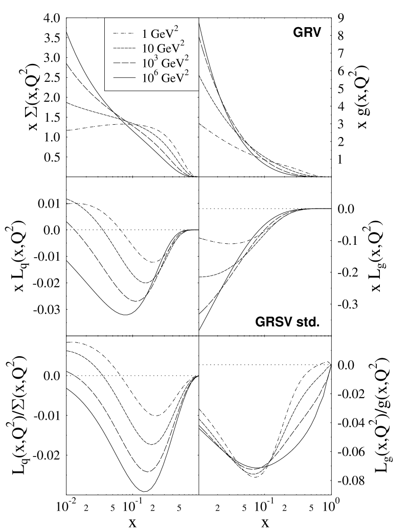
Figure 1: Evolution of orbital angular momentum. The GRSV LO standard scenario is used as input for the polarized parton distributions at $\mu_{0}^{2}=0.23$ GeV². At this scale the missing angular momentum of  0.025 units is evenly distributed among $L_{q}(x,\mu_{0}^{2})$ and $L_{g}(x,\mu^{2})$, which are assumed to have the same shape as $u_{v}(x,\mu_{0}^{2})$ and $g(x,\mu_{0}^{2})$, respectively.

Figure 2: Evolution of orbital angular momentum. The GRSV LO gmax scenario is used as input for the polarized parton distributions at $\mu_{0}^{2}=0.23$ GeV². The missing angular momentum of -0.43 units is evenly distributed among $L_{q}(x,\mu_{0}^{2})$ and $L_{g}(x,\mu^{2})$, which again are assumed to be proportional to $u_{v}(x,\mu_{0}^{2})$ and $g(x,\mu_{0}^{2})$, respectively.

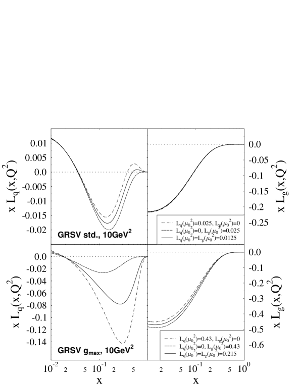
Figure 3: The missing angular momentum is distributed among $L_{q}(x,\mu_{0}^{2})$ and $L_{g}(x,\mu_{0}^{2})$ in three different ways, by setting the first moments of these distributions either equal or to 0.

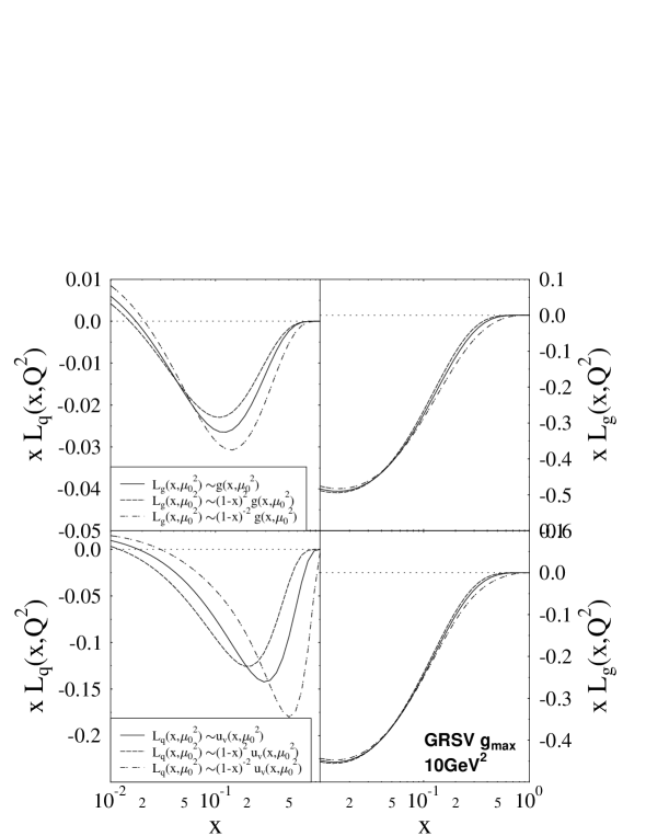
Figure 4: Dependence of the orbital angular momentum distributions on the shape of $L_{g}(x,\mu_{0}^{2})$ and $L_{q}(x,\mu_{0}^{2})$ at large $x$. $L_{q}(x,\mu_{0}^{2})$ ($L_{q}(x,\mu_{0}^{2})$) is set to 0 when $L_{g}(x,\mu_{0}^{2})$ ($L_{q}(x,\mu_{0}^{2})$) is varied.

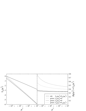
Figure 5: Evolution of the first moment of $L_{g}(x,\mu^{2})$ and the gluon contribution to the proton spin in different scenarios.

References

• [1] R.L. Jaffe and A. Manohar, Nucl. Phys. B337 (1990) 509
• [2] R.L. Jaffe and X. Ji, Phys. Rev. Lett. 67 (1991) 552
• [3] R.L. Jaffe and X. Ji, Nucl. Phys. B 375 (1992) 527
• [4] R.L. Jaffe, ’Spin,twist and hadron structure in deep inelastic processes’, in F. Lenz et al. (Eds) ’Lectures on QCD - Applications’, Graduiertenkolleg Erlangen-Regensburg, Springer 1997
• [5] R.L. Jaffe, Phys. Lett. B365 (1995) 359
• [6] S.V. Bashinsky and R.L. Jaffe, ’Quark and gluon orbital angular momentum and spin in hard processes’, preprint, hep-ph/9804397
• [7] X. Ji, J. Tang, and P. Hoodbhoy, Phys. Rev. Lett. 76 (1996) 740
• [8] X. Ji, Phys. Rev. Lett. 78 (1997) 610
• [9] P. Hoodbhoy, X. Ji, W. Lu, ’Quark orbital-angular-momentum distribution in the nucleon’, preprint, hep-ph/9804337
• [10] P. Hägler, A. Schäfer, preprint, Phys. Lett. B430 (1998) 179.
• [11] A. Harindranath and R. Kundu, ’On orbital angular momentum in deep inelastic scattering’, preprint, hep-ph/9802406
• [12] B.-Q. Ma and I. Schmidt, ’The quark orbital angular momentum in a light cone representation’, preprint, hep-ph/9808202
• [13] O.E. Teryaev, ’Evolution, probabilistic interpretation and decoupling of orbital and total angular momenta in nucleons’ preprint, hep-ph/9803403
• [14] M. Glück, E. Reya, A. Vogt, Z. Phys. C48, 471 (1990).
• [15] M. Glück, E. Reya, M. Stratmann, and W. Vogelsang, Phys. Rev. D53, 4775 (1996).
Refer to caption