Anomalous Magnetic and Electric Dipole Moments of the Tau
Invited talk at the TAU’98 Workshop, 14-17 September 1998, Santander, Spain

Abstract

This paper reviews the theoretical predictions for and the experimental measurements of the anomalous magnetic and electric dipole moments of the tau lepton. In particular, recent analyses of the ${\mathrm{e^{+}e^{-}\rightarrow\tau^{+}\tau^{-}\gamma}}$ process from the L3 and OPAL collaborations are described. The most precise results, from L3, for the anomalous magnetic and electric dipole moments respectively are: $a_{\tau}=0.004\pm 0.027\pm 0.023$ and $d_{\tau}=(0.0\pm 1.5\pm 1.3)\times 10^{-16}{e{\cdot}\mathrm{cm}}$.

1 INTRODUCTION

In the Standard Model (SM), the electromagnetic interactions of each of the three charged leptons are assumed to be identical, apart from mass effects. There is, however, no experimentally verified explanation for why there are three generations of leptons nor for why they have such differing masses. New insight might be forthcoming if the leptons were observed to have substructure which could manifest itself experimentally in anomalous values for the magnetic or electric dipole moments.

In general a photon may couple to a lepton through its electric charge, magnetic dipole moment, or electric dipole moment (neglecting possible anapole moments[1]). The most general Lorentz-invariant form for the coupling of a charged lepton to a photon of 4-momentum $q_{\nu}$ is obtained by replacing the usual $\gamma^{\mu}$ by

$$\Gamma^{\mu} = F_{1}(q^{2})\gamma^{\mu}$$ (1)

$$+ F_{2}(q^{2})\frac{i}{2m_{\ell}}\sigma^{\mu\nu}q_{\nu}-F_{3}(q^{2})\sigma^{\mu\nu}\gamma^{5}q_{\nu}.$$

The $q^{2}$-dependent form-factors, $F_{i}(q^{2})$, have familiar interpretations for $q^{2}=0$. $F_{1}(q^{2}\!=\!0)\equiv Q_{\ell}$ is the electric charge of the lepton. $F_{2}(q^{2}\!=\!0)\equiv a_{\ell}=(g_{\ell}-2)/2$ is the anomalous magnetic moment of the lepton. $F_{3}(q^{2}\!=\!0)\equiv d_{\ell}/Q_{\ell}$, where $d_{\ell}$ is the electric dipole moment of the lepton. Hermiticity of the electromagnetic current forces all of the $F_{i}$ to be real. In the SM $a_{\ell}$ is non-zero due to loop diagrams. A non-zero value of $d_{\ell}$ is forbidden by both $P$ invariance and $T$ invariance such that, if $CPT$ invariance is assumed, observation of a non-zero value of $d_{\ell}$ would imply $CP$ violation.

The anomalous moments for the electron and muon have been measured with very high precision and are in impressive agreement with the theoretical predictions, as shown in Table 1.

Table 1: Theoretical predictions and experimental measurements of the anomalous magnetic and electric dipole moments of the electron and muon.

$a_{\mathrm{e}}^{\mathrm{\scriptscriptstyle{SM}}}$	$=0.001\,159\,652\,46(15)$	[2]
$a_{\mathrm{e}}^{\mathrm{expt}}$	$=0.001\,159\,652\,193(10)$	[3]
$a_{\mu}^{\mathrm{\scriptscriptstyle{SM}}}$	$=0.001\,165\,920\,2(20)$	[4]
$a_{\mu}^{\mathrm{expt}}$	$=0.001\,165\,923\,0(84)$	[3]
$d_{\mathrm{e}}^{\mathrm{expt}}$	$=(-2.7\pm 8.3)\cdot 10^{-27}\,e\,{\mathrm{cm}}$	[5]
$d_{\mu}^{\mathrm{expt}}$	$=(3.7\pm 3.4)\cdot 10^{-19}\,e\,{\mathrm{cm}}$	[6]

In the SM $a_{\tau}$ is predicted to be $a_{\tau}^{\scriptscriptstyle{\mathrm{SM}}}=0.001\,177\,3(3)$ [7, 8]. The short lifetime of the tau precludes precession measurements which means that the tau cannot be measured with a precision comparable to those achieved for the electron and muon. Less precise experimental measurements of $a_{\tau}$ and $d_{\tau}$ using different techniques are nonetheless extremely interesting since they are sensitive to a wide variety of new physics processes.

The process $\mathrm{e}^{+}\mathrm{e}^{-}\rightarrow\gamma\rightarrow\tau^{+}\tau^{-}$ has been used to constrain $F_{2}$ and $F_{3}$ of the tau at $q^{2}$ up to $(37~{}\mathrm{GeV})^{2}$ [9], and an indirect limit has been inferred from the width $\Gamma(Z\rightarrow\tau^{+}\tau^{-})$ [10]. These results do not correspond to $q^{2}=0$ therefore the upper limits obtained on the form factors $F_{2}$ and $F_{3}$ do not correspond to constraints on the static tau properties, $a_{\tau}$ and $d_{\tau}$.

The process ${\mathrm{e^{+}e^{-}\rightarrow\tau^{+}\tau^{-}\gamma}}$, first analysed by Grifols and Mendez using L3 data [11], is attractive since $q^{2}=0$ for the on-shell photon. In this paper, we report on recent measurements of this process from the L3 and OPAL collaborations [12, 13]. These are based on analyses of ${\mathrm{e^{+}e^{-}\rightarrow\tau^{+}\tau^{-}\gamma}}$ events selected from the full LEP I on-peak data samples. No results are currently available from the ALEPH, DELPHI, or SLD collaborations.

2 THEORETICAL MODELLING

There are two published calculations of the process ${\mathrm{e^{+}e^{-}\rightarrow\tau^{+}\tau^{-}\gamma}}$, allowing for anomalous electromagnetic moments, that of Biebel and Riemann, which we refer to as “B&R” [14], and that of Gau, Paul, Swain, and Taylor which is known as “TTG” [15, 16].

L3 uses the TTG calculation while OPAL uses an unpublished calculation of D. Zeppenfeld, with an additional correction based on the B&R calculation.

2.1 Comparison of theoretical models

Both B&R and TTG parametrise the effects of anomalous dipole moments using the ansatz of Eq. 1 and calculate the squared matrix element for the process ${\mathrm{e^{+}e^{-}\rightarrow\tau^{+}\tau^{-}\gamma}}$. The TTG calculation is more complete than that of “B&R” and includes all the Standard Model and anomalous amplitudes for the diagrams shown in Figure 1.

The TTG matrix element, ${\cal{M}}(a_{\tau},d_{\tau})$, is determined without making simplifying assumptions. In particular, no interference terms are neglected and no fermion masses are assumed to be zero. The inclusion of a non-zero tau mass is essential, as the (significant) interference terms between the Standard Model and the anomalous amplitudes vanish in the limit of vanishing tau mass. Standard Model radiative corrections are incorporated by using the improved Born approximation.

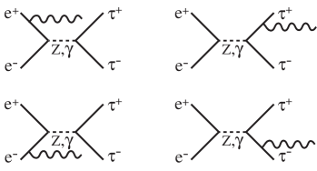
Figure 1: Diagrams contributing to $e^{+}e^{-}\rightarrow\tau^{+}\tau^{-}\gamma$ at tree-level.

Infrared divergences for collinear or low energy photons may be naturally avoided by applying cuts on minimum photon energy and/or opening angle between the photon and tau. This method eliminates potential concerns about the consistency of cancelling divergences against vertex corrections which are calculated in QED assuming that the anomalous couplings vanish. Moreover, this procedure matches well the experimental reality, since electromagnetic calorimeters have a minimum energy cutoff and isolation cuts are required to distinguish tau decay products from radiated photons.

The TTG calculation of ${\cal{M}}(0,0)$ is checked by comparison with the SM $O(\alpha)$ predictions of KORALZ. The shapes of the photon energy and angular distributions are in excellent agreement and the overall normalisation agrees to $0.1\%$.

The B&R calculation makes some reasonable approximations in order to arrive at a more manageable analytic expression, compared to the very complicated one provided by TTG. In particular, B&R neglects anomalous contributions to the ISR and FSR interference, $\gamma$ exchange, and $\gamma-$Z interference. To check the two calculations, the quantity $\Delta{\cal{M}}^{2}=|{\cal{M}}(a_{\tau},d_{\tau})|^{2}-|{\cal{M}}(0,0)|^{2}$ from TTG is compared to the prediction of B&R, using the same approximations in TTG as used in the B&R calculation. The anomalous contribution to the cross section agrees to better than $1\%$ [15] and the shapes of the photon energy spectra are in good agreement for a wide range of $a_{\tau}$ and $d_{\tau}$ values. The B&R calculation differs from the full TTG calculation by only 1% indicating that the neglect of certain terms in the B&R case is valid within the sensitivity of the LEP experiments.

Both calculations show that terms linear in $F_{2}(0)$ arise from interference between Standard Model and anomalous amplitudes. Figure 2 shows the contribution to the total cross section arising from these terms, with the linear and quadratic components shown separately [15]. The interference terms for $F_{2}(0)$ are significant compared to the total anomalous cross section for small values of $F_{2}(0)$. For example, for $F_{2}(0)=0.01$, inclusion of the linear terms enhances the number of excess photons, compared to the purely quadratic calculation, by a factor of approximately five. The anomalous contribution due to $F_{3}(0)$ is identical to the quadratic term for $F_{2}(0)$ in that the linear terms vanish identically.

Figure 2: Anomalous contribution to the $e^{+}e^{-}\rightarrow\tau^{+}\tau^{-}\gamma$ cross section as a function of $F_{2}(0)$ showing the linear and quadratic contributions.

2.2 Effects of anomalous couplings

Figure 3 shows the results of an OPAL Monte Carlo study of the photon energy spectrum, $\tau\tau$ acollinearity, and the polar angle of the photon in the laboratory frame for the SM, represented by the KORALZ Monte Carlo [17], and the shape of the additional anomalous contribution.

Figure 3: OPAL Monte Carlo study of a) the photon energy spectrum, b) the $\tau\tau$ acollinearity, and c) the polar angle of the photon in the laboratory frame for the SM (KORALZ) contribution and the arbitrarily-normalised anomalous contribution from a non-zero $F_{2}(0)$.

The anomalous electromagnetic moments tend to enhance the production of high energy photons which are isolated from the taus, compared to the SM final state radiation which has a rapidly falling energy spectrum of photons which tend to be collinear with one of the taus. The characteristics of the energy and angular distributions of ${\mathrm{e^{+}e^{-}\rightarrow\tau^{+}\tau^{-}\gamma}}$ events are exploited to enhance the sensitivity to anomalous moments, as described below.

2.3 Monte Carlo events samples

In order to study the various selection criteria and the backgrounds L3 and OPAL use large samples of Monte Carlo events, in particular: hadronic events from the JETSET Monte Carlo program [18]; two-photon events from DIAG36 [19] (L3) and VERMASEREN (OPAL) [13, ref. 17]; Bhabha events from BHAGENE [20] (L3) or RADBAB (OPAL) [13, ref. 17]; $\mu\mu(\gamma)$ and $\tau\tau(\gamma)$ events from KORALZ [21]. The KORALZ  samples include the effects of initial and final state SM bremsstrahlung corrections to $O(\alpha^{2})$ including exclusive exponentiation. All Monte Carlo events are passed through GEANT-based detector simulation programs, and reconstructed in the same way the data.

To model the effects of anomalous moments allowing for all SM, detector, and reconstruction effects the KORALZ samples of SM ${\mathrm{e^{+}e^{-}\rightarrow\tau^{+}\tau^{-}\gamma}}$ events are reweighted according to various assumed values of $F_{2}(0)$ and $F_{3}(0)$.

In the L3 case, TTG is used to determine a weight for each KORALZ event which depends on the generated four-vectors of the taus and the photon and on the values of $F_{2}(0)$ and $F_{3}(0)$ under consideration. This procedure takes full account of any dependences of the acceptance or reconstruction efficiency which arise from the kinematic variations of the event topologies with $F_{2}(0)$ and $F_{3}(0)$. Since TTG is an $O(\alpha)$ calculation, there is no unambiguous way to compute a weight for events with more than one photon. The treatment of multiple photon events is treated as a systematic error.

In the OPAL case, individual events are not reweighted. Instead, only the selected photon energy distribution is reweighted according to the naive Zeppenfeld predictions (which neglect interference completely) and a correction is then applied for the missing interference terms using the B&R prediction.

3 EXPERIMENTAL ANALYSIS

L3 and OPAL both analyse their full on-peak Z data samples which each correspond to an integrated luminosity of approximately 100 ${\mathrm{pb}}^{-1}$.

3.1 Event selection

L3 and OPAL first select a sample enriched in ${\mathrm{e^{+}e^{-}\rightarrow\tau^{+}\tau^{-}(\gamma)}}$ events by rejecting most of the hadronic, Bhabha, dimuon, two-photon, and other background events using reasonably standard selection cuts. Then, they identify photons above a few GeV in energy which are isolated from the decay products of the tau.

These events are in general very distinctive. For example, Figure 4 shows a typical $\tau\tau\gamma$ candidate event as seen in the L3 detector.

Figure 4: Typical $\tau\tau\gamma$ candidate event at L3.

The decay products of the taus in this event leave tracks in the inner tracker (TEC) and energy in the electromagetic (BGO) and hadron calorimeters. The photon has no associated track, leaves a considerable amount of energy in the BGO, and no energy in the hadron calorimeter.

L3 selects 1559 ${\mathrm{e^{+}e^{-}\rightarrow\tau^{+}\tau^{-}\gamma}}$ candidate events with a non-${\mathrm{\tau\tau\gamma}}$ background of 6.7% while OPAL selects 1429 events with a background of 0.13%. The Monte Carlo samples show that for both experiments the ${\mathrm{\tau\tau\gamma}}$ samples are dominated by genuine SM ${\mathrm{\tau\tau\gamma}}$ events. For example, SM processes are predicted to yield a sample of 1590 events in the L3 case. The significant difference in non-${\mathrm{\tau\tau\gamma}}$ background levels reflects differing severities of selection cuts. For example, OPAL uses electron momentum measurements in the tracker to reject residual Bhabha backgrounds, which is not done for the L3 analysis.

3.2 Determination of $F_{2}(0)$ and $F_{3}(0)$

Anomalous values of $F_{2}(0)$ and $F_{3}(0)$ tend to increase the cross section for the process ${\mathrm{e^{+}e^{-}\rightarrow\tau^{+}\tau^{-}\gamma}}$, especially for photons with high energy which are well isolated from the decay products of the taus. The information used in the fits to extract $F_{2}(0)$ and $F_{3}(0)$ are somewhat different for the two experiments as described below, although both L3 and OPAL conservatively set $F_{3}(0)=0$ when fitting for $F_{2}(0)$ and vice versa.

L3 makes binned maximum likelihood fits to the two-dimensional distribution of the photon energy, $E_{\gamma}$, vs. the angle between the photon and the closest tau jet, $\psi_{\gamma}$. To exploit the cross-section information, the SM Monte Carlo samples are normalised to the integrated luminosity. Figure 5 shows the L3 distributions of $E_{\gamma}$ and $\psi_{\gamma}$ for the data and the SM Monte Carlo expectation. Both the increase in the total cross section and the relatively greater importance of photons with large $E_{\gamma}$ and $\psi_{\gamma}$ are evident.

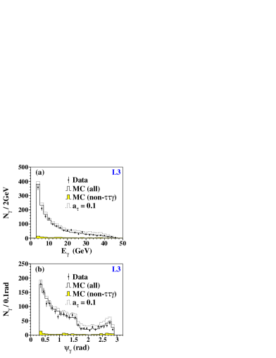
Figure 5: The number $N_{\gamma}$ of photon candidates in the L3 ${\mathrm{e^{+}e^{-}\rightarrow\tau^{+}\tau^{-}\gamma}}$ sample as a function of (a) $E_{\gamma}$ and (b) $\psi_{\gamma}$. The points with error bars denote the data and the solid histograms denote the SM Monte Carlo predictions. The dashed histograms show how the predictions for $a_{\tau}=0.1$.

No excess is apparent at high values as would be expected for significant deviations of $F_{2}(0)$ and/or $F_{3}(0)$ from their SM values. The results of the L3 fits to the data, considering only statistical errors, are $F_{2}(0)=0.004\pm 0.027$ and $F_{3}(0)=(0.0\pm 1.5)\times 10^{-16}e\cdot\mathrm{cm}$, where the errors refer to the $68.3\%$ confidence interval. These two results are not independent, although the absence of interference terms for $d_{\tau}$ does provide some distinguishing power between the effects of $a_{\tau}$ and those of $d_{\tau}$ [15].

OPAL makes a one-dimensional fit to the energy spectrum of the photons. The total cross-section information is not used since the normalisation of data and Monte Carlo are forced to agree. Although there is some loss of sensitivity as a result, there is a negligible systematic error from uncertainties in the photon reconstruction efficiency. Figure 6 shows the OPAL distributions of photon energy for the data and the SM Monte Carlo expectation.

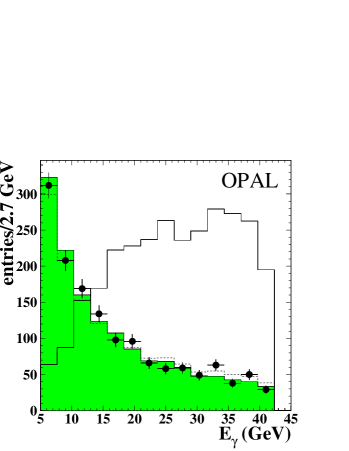
Figure 6: The number of photon candidates in the OPAL ${\mathrm{e^{+}e^{-}\rightarrow\tau^{+}\tau^{-}\gamma}}$ sample as a function of $E_{\gamma}$. The points with error bars denote the data and the filled solid-line histogram denotes the SM prediction. The dashed histogram shows the expectation for $F_{2}(0)=0.064$. The un-filled solid-line histogram shows, with arbitrary normalisation, the signal expectation only.

The OPAL result for $F_{2}(0)$, after correction for the effects of interference, is $0.065<F_{2}(0)<0.062$ at the 95% confidence level. The value of $F_{3}(0)$ is not fitted directly but is inferred from the $F_{2}(0)$ analysis, as described below.

3.3 Systematic errors

Both L3 and OPAL perform numerous cross-checks of their analyses using independent data samples and the Monte Carlo samples. The various contributions to the systematic errors on $F_{2}(0)$ are described below, those for $F_{3}(0)$ are similar.

It is important to note that while L3 quotes individual systematic errors in the conventional ($\pm 1\sigma$) way, the OPAL values correspond to estimated changes in the 95% limit and are hence numerically much smaller in general. To make this distinction clear, we denote the former by $\sigma^{\mathrm{L3}}(F_{2})$ and the latter by $\delta_{95}^{\mathrm{OPAL}}(F_{2})$.

• Event selection cuts
  Wide variations in the selection cuts yield systematics of $\sigma^{\mathrm{L3}}(F_{2})=0.013$ and $\delta_{95}^{\mathrm{OPAL}}(F_{2})=0.005$.

• $\tau\tau(\gamma)$ selection efficiency
  To verify the ${\mathrm{e^{+}e^{-}\rightarrow\tau^{+}\tau^{-}(\gamma)}}$ event selection efficiency, L3 determines the ${\mathrm{e^{+}e^{-}\rightarrow\tau^{+}\tau^{-}(\gamma)}}$ cross-section at $\sqrt{s}\approx m_{\mathrm{Z}}$ to be $\sigma_{\tau\tau}=(1.472\pm 0.006\pm 0.020)\,{\rm{nb}}$, in agreement with the SM prediction of ZFITTER [22] of $1.479{\rm{\,nb}}$. This indicates the absence of significant systematic effects in the selection of taus and contributes an error of $\sigma^{\mathrm{L3}}(F_{2})=0.011$.

  OPAL is relatively insensitive to this source of uncertainty since the normalisation of the data and Monte Carlo is enforced (resulting in a loss of statistical sensitivity).

• Photon reconstruction efficiency
  L3 performed a particularly compelling analysis of ${\mathrm{e^{+}e^{-}\rightarrow\mu^{+}\mu^{-}\gamma}}$ events selected from the data and compared to Monte Carlo predictions, which are known to have no significant anomalous effects. Figure 7 shows the distributions of photon energy $E_{\gamma}$ and the isolation angle $\psi_{\mu\gamma}$ of the photon to the closest muon in the selected $\mu\mu\gamma$ event sample. The data are in good agreement with the Monte Carlo prediction. The ratio of the number of photons in data to the number in the Monte Carlo is $0.993\pm 0.013\pm 0.003$. The shapes of the energy and isolation distributions also agree well, with $\chi^{2}/NDF=50.2/44$ for the former and $\chi^{2}/NDF=37.6/30$ for the latter, based only on the statistical error.

  

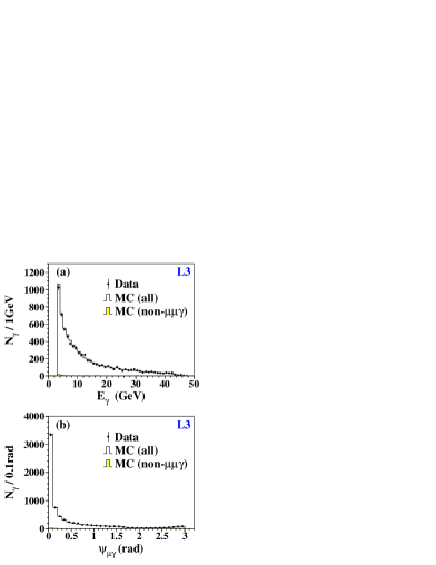
  Figure 7: The number $N_{\gamma}$ of photon candidates in the ${\mathrm{e^{+}e^{-}\rightarrow\mu^{+}\mu^{-}\gamma}}$ sample as a function of (a) $E_{\gamma}$ and (b) $\psi_{\mu\gamma}$. The points with error bars denote the data and the histograms denote the Monte Carlo predictions.

  The uncertainty on the photon reconstruction efficiency yields an error of $\sigma^{\mathrm{L3}}(F_{2})=0.010$, which is conservative since some effects are covered by the variation of the selection cuts.

  OPAL is relatively insensitive to this source of uncertainty since the normalisation of the data and Monte Carlo is enforced.

• Backgrounds
  The L3 error due to uncertainties in the non-${\mathrm{\tau\tau\gamma}}$ backgrounds is $\sigma^{\mathrm{L3}}(F_{2})=0.009$. By comparison, OPAL has negligible uncertainty due to their lower level of non-${\mathrm{\tau\tau\gamma}}$ background.

• Binning
  The selected samples are fitted using a variety of binning schemes, to yield $\sigma^{\mathrm{L3}}(F_{2})=0.008$ for the two-dimensional L3 fit and $\delta_{95}^{\mathrm{OPAL}}(F_{2})=0.002$ for the one-dimensional OPAL fit.

• Photon energy scale and resolution
  L3 studies electrons in ${\mathrm{e^{+}e^{-}\rightarrow e^{+}e^{-}(\gamma)}}$, ${\mathrm{e^{+}e^{-}\rightarrow\tau^{+}\tau^{-}(\gamma)}}$, and ${\mathrm{e^{+}e^{-}e^{+}e^{-}}}$ events, pairs of photons from $\pi^{0}$ decays, and pairs of electrons from $J/\psi$ decays. The photon energy scale uncertainty is $<$0.5% for $E_{\gamma}\approx 3$ GeV and $<$0.05% for $E_{\gamma}\approx m_{\scriptscriptstyle{\mathrm{Z}}}/2$. The resolution is $(1.7\pm 0.3\%)$ at $E_{\gamma}\approx 10$ GeV and $(1.4\pm 0.1)\%$ for $E_{\gamma}\approx m_{\scriptscriptstyle{\mathrm{Z}}}/2$. Allowing for theses uncertainties yields $\sigma^{\mathrm{L3}}(F_{2})=0.008$. The ${\mathrm{\mu\mu\gamma}}$ study also confirms the absence of significant systematic uncertainties in the photon energy measurement.

  OPAL verifies their energy scale somewhat less precisely (0.9%) using $\pi^{0}$ decays and estimates an effect of $\delta_{95}^{\mathrm{OPAL}}(F_{2})=0.001$. They do not quote a systematic error from uncertainties in the photon energy resolution.

• Modelling of ${\mathrm{e^{+}e^{-}\rightarrow\tau^{+}\tau^{-}\gamma}}$
  The inclusion by L3 of the ${\mathrm{\mu\mu\gamma}}$ error allows for possible systematics in the KORALZ description of SM photon radiation. The TTG calculation of ${\cal{M}}(0,0)$, used by L3, agrees with the $O(\alpha)$ predictions of KORALZ to within $0.1\%$. The TTG calculation of $|{\cal{M}}(a_{\tau},d_{\tau})|^{2}$ agrees, for the same approximations, with the B&R calculation [14] to better than $1\%$ [15]. Variation of the TTG predictions within these uncertainties causes a negligible change in the L3 fit results.

  OPAL does not explicitly comment on this potential source of systematic uncertainty.

• Multiple photon radiation
  To estimate the effects of multiple photon radiation in the L3 analysis, KORALZ is used to generate a sample of ${\mathrm{e^{+}e^{-}}}\rightarrow\tau^{+}\tau^{-}(n\gamma)$ events. Then all photons, except for the one with the highest momentum transverse to the closer tau, are incorporated into the four-vectors of the other particles in such a way that all particles remain on mass shell [16]. Weights for various $a_{\tau}$ and $d_{\tau}$ are then computed by TTG using the modified four-vectors of the taus and the photon. Taking these weights in lieu of those computed using the previously described method, in which only events with a single hard photon are considered, has a negligible effect on the result of the fit.

  OPAL does not explicitly comment on this potential source of systematic uncertainty.

4 SUMMARY

The systematic errors described above are combined, to yield the L3 fit results for $a_{\tau}$ and $d_{\tau}$:

$$a_{\tau} = 0.004\pm 0.027\pm 0.023$$ (2)

$$d_{\tau} = (0.0\pm 1.5\pm 1.3)\times 10^{-16}e\cdot\mathrm{cm}$$ (3)

where the first error is statistical and the second error is systematic. These correspond to the following limits:

$$-0.052<a_{\tau}<0.058~{}~{}~{}{\mathrm{and}}$$ (4)

$$|d_{\tau}|<3.1\times 10^{-16}e\cdot\mathrm{cm}$$ (5)

at the 95% confidence level.

OPAL chooses to quote 95% confidence level limits only. Their result is

$$-0.068<a_{\tau}<0.065.$$ (6)

If interference is neglected, the calculations for the magnetic and electric dipole moments are equivalent. Therefore, OPAL makes the substitution: $F_{2}/2m_{\tau}\longrightarrow F_{3}$. to convert their constraints on $|F_{2}|$ to a constraint on $F_{3}$:

$$|d_{\tau}|<3.7\times 10^{-16}e\cdot\mathrm{cm}.$$ (7)

The OPAL results are comparable with the slightly more precise L3 results. Both are consistent with the SM expectations and show no evidence for the effects of new physics.

References

- [1] W. J. Marciano. 1990. Proceedings of the BNL Summer Study on CP Violation, Brookhaven National Laboratory, eds. S. Dawson and A. Soni.
- [2] T. Kinoshita and W. B. Lindquist. Phys. Rev. Lett., 47:1573, 1981.
- [3] E. R. Cohen and B. N. Taylor. Rev. Mod. Phys., 59:1121, 1987.
- [4] V. W. Hughes and T. Kinoshita. Comm. Nucl. and Part. Phys., 14:341, 1985.
- [5] K. Abdullah et al. Phys. Rev. Lett., 65:2347, 1990.
- [6] J. Bailey et al. Journ. Phys., G4:345, 1978.
- [7] G. Li M. A. Samuel and R. Mendel. Phys. Rev. Lett., 67:668, 1991. Erratum ibid 69 (1992) 995.
- [8] F. Hamzeh and N.F. Nasrallah. Phys. Lett., B373:211, 1996.
- [9] D. J. Silverman and G. L. Shaw. Phys. Rev., D27:1196, 1983.
- [10] R. Escribano and E. Massó. Phys. Lett., B395:369, 1997.
- [11] J. A. Grifols and A. Méndez. Phys. Lett., B255:611, 1991. Erratum ibid B259 (1991) 512.
- [12] L3 Collab., M. Acciarri et al. Phys. Lett., B434:169, 1998.
- [13] OPAL Collab., K. Ackerstaff et al.. Phys. Lett., B431:188, 1998.
- [14] J. Biebel and T. Riemann. Z. Phys., C76:53, 1997.
- [15] S.S. Gau, T. Paul, J. Swain, and L. Taylor. Nucl. Phys., B 523:439, 1998.
- [16] T. Paul and Z. Wa̧s. hep-ph/9801301.
- [17] B.F.L. Ward S. Jadach and Z. Wa̧s. 66:276, 1991.
-
[18]
T. Sjöstrand, Comp. Phys. Comm. 39 (1986) 347;
T. Sjöstrand and M. Bengtsson, Comp. Phys. Comm. 43 (1987) 367. - [19] F.A. Berends, P.H. Daverveldt and R. Kleiss. Comp. Phys. Comm., 40:285, 1986.
-
[20]
J. H. Field, Phys. Lett. B 323 (1994) 432;
J. H. Field and T. Riemann, Comp. Phys. Comm. 94 (1996) 53. - [21] S. Jadach, B. F. L. Ward and Z. Wa̧s. Comp. Phys. Comm., 79:503, 1994. KORALZ uses TAUOLA to decay the taus (see: S. Jadach, J.H. Kühn and Z. Wa̧s, Comp. Phys. Comm. 64 (1991) 275) and PHOTOS for multiple photon radiation (see: E. Barberio, B. van Eijk and Z. Wa̧s, Comp. Phys. Comm. 66 (1991) 128).
-
[22]
D. Bardin et al., FORTRAN package ZFITTER, and preprint CERN–TH. 6443/92;
D. Bardin et al., Z. Phys. C 44 (1989) 493;
D. Bardin et al., Nucl. Phys. B 351 (1991) 1;
D. Bardin et al., Phys. Lett. B 255 (1991) 290.