Geometrical pictures for the family structure of fundamental particles are developed. They indicate that there might be a relation between the family repetition structure and the number of space dimensions.

1. Introduction

With the discovery of the top quark all in all 12 fundamental fermions (6 leptons and 6 quarks) are known today. At least a decade ago it has become clear that these particles can be organized into three ”families” each containing 2 quarks and 2 leptons. These particle families (or generations) behave identically under the electroweak and strong interactions and do not differ by anything else than their masses. The number of generations will probably be restricted to three forever, because it has been shown experimentally that at most 3 species of light neutrinos exist. A fourth family,if it exists at all, would necessarily contain a heavy neutrino and would therefore be different in nature from the known families.

Over the last 20 years there has been one outstanding puzzle in elementary particle physics. This is the question whether the variety of ”elementary” particles, the quarks and leptons, can be derived from some more fundamental principle. To answer this question is quite difficult because up to now no experimental indications exist of which might be the nature of this principle. Present models usually lead to an inflation of new particles (like supersymmetry) at higher energies and/or tend to shift the basic problems to higher energy scales where they reappear in slightly modified form (like technicolor).

Preon models (e.g. [2]) avoid these deficiencies but have severe problems of other kinds, like the smallness of fermion masses as compared to the binding scale. Still, I want to follow in this work a preon type idea, that the quarks and leptons have a spatial extension, and contain most probably sub–constitutents. My guideline will be that the spatial dimensions correspond to a sort of shells which are successively filled up by the generations. The third shell – corresponding in some sense to the third dimension – becomes closed with the top quark. Several ”pictures” will be presented which en gross adhere to this general philosophy but differ in the details of its realization. I shall also address the question of how to understand the vector bosons and the mass hierarchy.

I shall make use of some discrete, nonabelean subgroups of O(3), in particular the symmetric group $S_{4}$. Discrete subgroups have been repeatedly studied in the literature to tackle the generation problem. However, the approach to be followed here is much different. For example, a spatial extension of the fermions will be assumed.

I would like to warn the reader that in this article I am mostly doing simple minded geometry without really clarifying the mathematics behind it. There are all sorts of unanswered questions concerning the dynamics of the model. My hope is that I can motivate readers to do more refined work on the basis of these suggestions.

2. The Family Repetition

The known quarks and leptons within one family are:

$$\nu_{L,R}\qquad e_{L,R}\qquad u^{1,2,3}_{L,R}\qquad d^{1,2,3}_{L,R}$$ (1)

where the upper index denotes the quark color degrees of freedom and the lower index the helicity. I have assumed here that a righthanded neutrino $\nu_{R}$ exists, because it exists naturally in most of the pictures developed below. Of course, one can very well have parity violation and righthanded neutrinos just by demanding that the observed W and Z only interact with lefthanded currents. However, one encounters new heavy vector bosons ($W_{R}$ and $Z_{R}$) to interact with the righthanded neutrino.

There are $2_{spin}\times 2_{isospin}\times(1+3_{color})=16$ degrees of freedom in one family (32, if antiparticles are counted as well) and altogether 48 degrees of freedom in all three generations. This might be related to a property of 3–dimensional space, namely that there are 48 symmetry transformations which leave the 3–dimensional cube invariant. Furthermore, as will be shown later, there are subgroups of this symmetry group which can be arranged in such a way that they look like the quark–lepton arrangement in the 3 families. Although this may be just by accident, I will explore in this article the implications of such a relation.

Any of the following models should have the ability to generate the quantum numbers of the observed fermions in a correct way. For example, the electric charges should come out correctly as multiples of one third because this is one of the main requirements which leads one to conclude that quarks and leptons are of the same origin.

It is well–known that up- and down type quarks take part in all the standard interactions (strong and electroweak) whereas the leptons do not couple strongly, and the neutrinos couple only weakly. These facts are reflected by the quantum numbers; neutrinos carry only the (weak) isospin, electrons an electric charge in addition, and quarks carry a color charge, an electric charge and a nontrivial weak isospin quantum number. The fact that neutrinos interact only weakly, is probably related to their tiny masses, and indicates that their ”sub–shells” are somewhat more closed than those of the other fermions. Similarly, since no lepton interacts strongly, they should be considered more saturated bound states than the quarks.

One might think that some information on the nature of the fermions can be obtained from their measured mass spectrum. However, the fermion masses are running, i.e. energy dependent, and it is not really known which dynamics governs this energy dependence. In other words, their enormalization group equations are not known precisely and therefore no complete knowledge of the fermion mass spectrum exists. For instance, the masses could be running according to some SUSY–GUT theory. However, apart from the fact that the SUSY breaking scale is not known precisely, new physics may set in at some point and modify the RG equations. Therefore it is not known to what values the fermion masses are converging. There might be relations like $m_{b}=m_{\tau}$ at scales $\sim 10^{16}$ GeV, but those are not compelling.

I think it is fair to say that we only have a rough knowledge of the fundamental mass parameters. The fermion mass spectrum is at most a qualitative guideline to understand the family structure.

As compared to the unification scale the masses of the known fermions are tiny. However, if compared among themselves the mass differences between the families and also within one family are so vastly different that one should work with mass ratios instead of mass differences to describe them. In spite of the above mentioned principle limitations one can sort out a few basic masses and ratios which will probably survive the RG running. Among them there is the ”overall mass” of a family, i.e. the average mass of its non–neutrino components. One has roughly

$$m_{I}=10^{7}\qquad m_{II}=10^{9}\qquad m_{III}=10^{11}$$ (2)

(in eV) for the first, second and third family, i.e. a factor of about 100 between the masses of successive generations.

Secondly there is the ratio between the neutrino and the average family mass $m_{F}$, which may be either zero or of the order

$${m_{\nu F}\over m_{F}}=10^{-10}\qquad,F=I,II,III$$ (3)

according to recent neutrino data and its smallness should be qualitatively explained by any model.

There are, thirdly, two less reliable mass ratios which I call X and Y and which arise if one looks at the approximate mass values of the fermions in the three generations. Namely, one realizes that the mass ratios

$$X\equiv{m_{\mu}\over m_{e}}\sim{m_{c}\over m_{u}}\sim{m_{t}\over m_{c}}\sim 200$$ (4)

are approximately equal. The same holds true for

$$Y\equiv{m_{\tau}\over m_{\mu}}\sim{m_{b}\over m_{s}}\sim{m_{s}\over m_{d}}\sim 20.$$ (5)

These relations are visualized in fig. 1. Admittedly they are very rough and could be spoiled by RG running, but they are interesting enough to be shown. I have included in fig. 1 an educated guess concerning the neutrino mass ratios. Starting from a mass $m(\nu_{\tau})=0.2$eV one is lead to $m(\nu_{\mu})\approx 0.001$eV and $m(\nu_{e})\approx 0.00005$eV which is in accord with recent results from solar–neutrino and Super–Kamiokande data.

Figure 1: Approximate mass ratios X and Y between particles of identical quantum numbers in successive generations. The numbers in brackets are the approximate fermion masses (in MeV) which lead to these mass ratios. The neutrino mass ratios are guessed.

To fully understand the fermion masses a detailed knowledge of the dynamics inside the fermions would be necessary. The models to be presented in this work are not able to provide this. It would already be progress if some qualitative features like the smallness of the neutrino masses as compared to the other fermions could be explained. Furthermore, there is the puzzle that all observed fermion masses are much smaller than the scale at which they are bound. t’Hooft [3] has suggested to decree chiral invariance as the principle which suppresses the fermion masses, and from this has derived conditions on the anomaly structure of the preon model. In the present work this is not a necessary condition. The point is that the extension of the observed fermions is not fixed by the binding energy of a superstrong force but by the structure of space. For example, in the model presented in section 5, space is essentially discrete with preons sitting on the sites of a cubic lattice. I shall stick to the notion of ’binding energy’, though, to mean the inverse extension of the ’bound states’. Actually, the binding energy is the scale at which the fermion masses should be defined.

For experiments at high energies the precise values of the fermion masses become less relevant. The only masses of actual significance at medium and high energies $(\geq m_{W})$ are $m_{W}$, $m_{t}$ and $m_{H}$. For practical purposes all the other masses may be put to zero. It would be extremely interesting if a mass relation of the form

$${m_{H}\over m_{W}}=G({m_{t}\over m_{W}})$$ (6)

would exist. Unfortunately, the Higgs particle is not a very natural object in the models to be presented. It may be constructed in some of the models, along similar lines as the vector bosons, but its existence is not compelling. To guarantee renormalizability of the low energy theory at small distances one should probably take it in.

3. Basic Assumptions

The basic assumption in this work goes as follows: the fermions in the first family can be considered as effectively one–dimensional objects composed of a shell which is successively filled up when one goes from the electron–neutrino to the up–quark. This is not to say that they are truely one–dimensional, but that their structure can be encoded in such a way as to correspond to one of the three spatial dimensions. We shall have several examples for that below.

The closed first family shell survives in the second family where another shell is beginning to fill. The second family is thus becoming 2–dimensional in nature. Finally, the third family fills 3-dimensional space completely. The structure is completed with the top quark. ’Completeness’ does not necessarily correspond to a saturation in the sense that the top quark mass would be lowered by the fact that the top quark corresponds to a closed shell. On the contrary! The particles mostly ’saturated’ are certainly the neutrinos, because their masses are extremely small and they interact only weakly. The models to be presented try to take that into account.

To account for the rather large mass difference between the overall family masses (factors $\sim 100$) one may speculate that they arise from ”exciting” the successive dimensions.

In most of the models considered below, preons are naturally assumed to be massless, or – less restrictive – have masses much smaller than their binding energy. Some of the vastly different masses of fermions may be due to preons of different mass, though. For example, to account for the extremely large mass difference between the neutrinos and quarks within one generation (a factor of order $10^{9}$ at least) one may introduce some sort of sub–quark present in quarks (and non-neutrino leptons) but not in neutrinos. This picture is more in accord with t’Hooft’s chiral invariance condition, where the difference in the observed fermion masses is attributed to the fact that the preons have different masses, and not to the (large) binding energy.

At first sight the large mass ratios between the families and also within one family make it difficult to believe that all particles can be derived from a universal symmetry principle. Still, all these masses are probably small as compared to the binding energy of the approximately massless preons.

In section 4 some qualitative pictures are developed to understand the connection between space and family. The model to be discussed most extensively will be presented afterwards in sections 5 and 6. There the existence of families will be tied to the 3 spatial dimensions, but instead of shells in the narrow sense we shall have 4 preons interacting with each other in various permutations, the set of all permutations ($S_{4}$) exhausting the fermionic and bosonic degrees of freedom. The preons will be sitting in the corners of a tetrad, to form a fermion. A vector boson can be obtained by fusion of 2 such tetrads to form a cube.

4. Some qualitative Pictures and Guidelines

In the following I want to develop a simple picture based on the 3–dimensional structure of space. To form the first generation, only one axis (’x’) is populated. To build up the second family the y–direction is filled up , etc. An example of how this may work, is shown in fig. 2. The fermions of the first generation are made up from two preons, drawn as full dots in fig. 2, and bound by forces which can be visualized as three, two or one lines connecting the presons. The graphs in fig. 2 with one, two or three lines connecting the presons correspond to $\nu_{e}$, $e$ and $u,d$, repectively. As another rule we demand that there are exactly 4 lines connecting to each preon. As a consequence, $\nu_{e}$, $e$ and $u,d$ have two, four and six open, ’unsaturated’ strings, respectively, cf. fig. 2.

Figure 2: a 1–dimensional ordering of the first family fermions.

It should be noted that a particle exists in this picture, which is completely saturated and therefore does not take part in any of the known interactions – apart from, perhaps, gravity. This particle is shown in the lower part of fig. 2. If it has a (tiny) mass, it would be a ’singlet’ type dark matter candidate.

The second generation is formed by doing the same construction as done for the first, but along the y–direction. The procedure for the second family ends when the singlet state is formed along the y–direction. Note that one starts with quarks in fig. 2, and goes via leptons and neutrinos, to the singlet state. It will be assumed that the singlet along the x–direction is present in all second (and third) family fermions, so that the second family is of 2–dimensional nature.

Finally, the third generation is made up along the z–direction, according to the same rules depicted in fig. 2. Note that in the third family the x– and y–direction are occupied by the first and second family singlet states and that the third generation fills 3–dimensional space completely.

In this picture weak,electromagnetic and strong interactions are a question of the number of open strings emerging from a preon. The strong interaction occurs when three open lines join together to form a bound state, for the electromagnetic interaction two lines are needed and for the weak interaction only one line of a lepton or quark connects with one line of another lepton or quark.

An important question is how the multiplicity of quarks arises. We have one lepton degree of freedom for each of the first pictures in fig. 2, but six quarks corresponding to the third picture in fig. 2. One possibility is to make a rule which counts the number of ways the open strings of one fermion can be connected. There is one possibility for the neutrino ($\nu_{L}$), two for the other leptons ($l_{L,R}$) and 6 for the quarks. Interaction processes like $\nu\bar{\nu}\rightarrow q\bar{q}$ may be understood as rearrangement of open and closed strings.

Furthermore, there is the question of how the fermion masses can, at least qualitatively, be understood. One can either try to understand them dynamically, from the magnitude of the fermion binding energies. Another possibility is to put a third, massive, preon into the centre of the electron and quarks, but not the neutrino.

The presented picture is not very sophisticated and certainly not complete. It is meant as a warming up for the more elaborate model to follow in section 5 and as a qualitative guideline of how families can be related to three spatial dimensions.

There are a lot of variations of the model presented here. For example, instead of constructing the fermions of one family by aligning the preons along spatial axes, one could align them in the 3 planes orthogonal to the coordinate axes, cf. fig 3. In such a picture one could, for example, put 4 identical preons $a$ on the corners of a square in the ’first family plane’, cf. fig. 3, and, perhaps, another (massive) preon in the centre of the square (except for the neutrinos). If $a$ has a quantum number which can take values $\pm 1$, one can form the 16 states necessary to build up a family. Note that in this picture there would be a right handed neutrino.

Figure 3:

Alternatively, one may develop a more dynamical picture in which two preons (with certain quantum numbers, to get the complete 16plet of fermions of the first generation) encircle each other in the first family plane. As for the second family, there are 2 other preons encircling each other in a plane orthogonal to the first one, etc.

Clearly, all of these pictures give no proof of the claim that the number of generations is tied to the number of dimensions. There is a more sophisticated picture in section 5 which might serve a better job. It centres around discrete subgroups of O(3). Of particular relevance will be the group of permutations $S_{4}$ which is isomorphic to the symmetry group of the tetrad. The discussion will concentrate on the subgroups themselves and not on their representations. This is a somewhat unusual approach, because normally in physics particle multiplets are identified with the representation spaces and not with the symmetry groups themselves. In contrast, the philosophy here is that by applying the symmetry transformations on the ground state ($\nu_{e}$) one can generate all other fermion states. This is only possible if there is a symmetry breaking which distinguishes the generated states. Such a symmetry breaking will be realized by geometrical means in the following section. To show how this can happen, I have visualized in fig. 4 an element of $S_{3}$, the permutation symmetry of the three sides of an equilateral triangle in 3 dimensions, assuming the existence of distinct preons A,B,C on the sites and distinct binding forces on the links of the triangle. If the $S_{3}$–transformation is applied to the sites but not to the links of the triangle, a completely different state is generated. In this case there are 6 such states corresponding to the 6 elements of $S_{3}$, which may have a relation to the weak vector bosons (see section 5).

Figure 4:

5. The Model

The following picture rests on the geometry of squares and cubes. The idea is to associate a particle degree of freedom to each of the symmetry transformations. In the case of squares there are 16 such transformations, among them the trivial unit operation, whereas for cubes there are 48.

As a warming up consider the set $S_{s}$ of symmetry transformations of the square embedded in 3–dimensional space. This yields a formal describtion of a one–family situation, in the following sense: It consists of 16 elements and is a direct product of the parity transformation $P\equiv(\vec{x}\rightarrow-\vec{x})$ with the set $D_{4}$ of 8 rotations depicted in fig. 5, $S_{s}=P\oplus D_{4}$. In fig. 5, $C_{n}$ stands for a rotation by $2\pi/n$ with the rotation axis being indicated. The parity transformation is clearly destinated to correspond to the two possible helicities of fermions. The lefthanded neutrino is taken to correspond to the unity transformation. All other fermion states within one family can be obtained from it by applying a nontrivial element of $S_{s}$.

The elements of $D_{4}$ are identified as the lefthanded fermions of the first generation

$$1(\nu_{L}),C_{4}^{2}(u_{L}^{1}),C_{4}(u_{L}^{2}),C_{4}^{3}(u_{L}^{3}),C_{2a}(e_{L}),C_{2b}(d_{L}^{1}),C_{2c}(d_{L}^{2}),C_{2d}(d_{L}^{3})$$ (7)

Clearly, as yet this is not much more than a schematic representation of what we already know to be the content of one family but we shall see that it is part of a more natural and larger scheme which contains the fermions of all generations. Namely, one can extend the consideration from 1 to 3 families by going from the square to the cube (with 3 planes, cf. fig 3). The symmetry group of the cube is the octahedral group $O_{h}$. It is also of a direct product form $O_{h}\equiv P\oplus S_{4}$ with $S_{4}$ being the group of symmetry transformations of the tetrad, sometimes also called $T_{h}$ or $O$ (where the $O$ stands for the octahedron whose transformations it also describes). $O_{h}$ contains exactly the 48=2x24 elements needed for a one to one correspondence with the particles of the 3 families. The philosophy here is that by applying the 48 symmetry transformations of the cube on one of the 48 fermion states one can generate all the other 48 fermion states. This indicates that the fermions should have some 3 dimensional substructure which completely breaks the symmetry of the cubic. Such a symmetry breaking can be realized in a variety of different ways as will be shown now.

Figure 5: The symmetry transformations in $D_{4}$.

The symmetry group $S_{4}$ of a tetrad is isomorphic to the group of permutations of 4 objects. This way the 24 symmetry tansformations on a tetrad can be viewed as the set of all (directed, open) paths that connect the 4 corner points 1,2,3,4 of the tetrad. From the tetrad a cube can be generated by applying the parity transformation. In fact there are two tetrads, a ’lefthanded’ (with corner points 1,2,3,4) and a ’righthanded’ (with corner points 1’,2’,3’,4’) embedded in a cube. (cf. fig. 6) related by P.

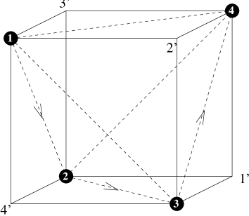
Figure 6: The ’lefthanded’ tetrad inside the cube. The path $1\rightarrow 2\rightarrow 3\rightarrow 4$ corresponding to the identity is marked by arrows.

From now on I will follow the philosophy that the spatial structure of a fermion (quark or lepton) is that of a tetrad. Furthermore, I assume that by applying the 24 symmetry transformations of the tetrad state one can create all 24 fermion states of the three families out of one of these states. In order to guarantee that all of the symmetry transformations yield different states, the tetrad cannot be completely symmetric. For example, one may assume that there are 4 different preons sitting on the 4 corners of the tetrad. Another possibility is that the preons are identical, but the binding forces between them are different. In the following we shall pursue this latter option. More specifically, we shall assume that the bindings between the 4 preons are given according to the 24 permutations of the set 1,2,3,4. One of the 24 permutations (namely the identity element) is visualized in fig. 6 by the 3 arrows $1\rightarrow 2\rightarrow 3\rightarrow 4$. Any other element $1234\rightarrow abcd$ of $S_{4}$, denoted by $\overline{abcd}$ in the following, could be drawn as the path $a\rightarrow b\rightarrow c\rightarrow d$ in fig. 6.

Starting with the ’lefthanded’ tetrad, one can construct all the 24 lefthanded fermion states of the 3 generations. By applying the parity transformation $(x,y,z)\rightarrow(-x,-y,-z)$, righthanded fermions can be obtained. Any such righthanded state will be denoted by $\overline{a^{\prime}b^{\prime}c^{\prime}d^{\prime}}$ in the following. As well known, a (Dirac) fermion $f$ has four degrees of freedom, of which only two, $f_{L}$ and $f_{R}$, have been described so far. The way to obtain antiparticles $\bar{f}_{L}$ and $\bar{f}_{R}$ is as follows: $\bar{f}_{L}$ is a righthanded object and its preons should therefore form a righthanded tetrad $\overline{a^{\prime}b^{\prime}c^{\prime}d^{\prime}}$ with field values corresponding not to $f_{R}$ but to the complex conjugate of $f_{L}$. Similarly, $\bar{f}_{R}=\overline{abcd}$ with field values which are complex conjugate to $f_{R}$.

As a side remark note that there might be something in the tetrad’s centre, but this is not modified by $S_{4}$ nor parity transformations (cf. footnote 1 below).

Let us now explicitly relate the elements of $S_{4}$ to the various members of the 3 generations. The geometrical model fig. 6 naturally suggests a separation of the 24 permutations into 3 subsets. To see this, look at the figures 8, 9 and 10, where the 3 possible closed paths which connects the points 1,2,3 and 4 are shown. These closed paths consist of 4 links. Permutations lying on the path I (fig. 8) will be attributed to the members of the first family, permutations on path II (fig. 9) to the second family and path III (fig. 10) to the third family. For example, look at the lefthanded states of the first family

$$\nu_{L} = \overline{1234}\qquad u^{1}_{L}=\overline{2341}\qquad u^{2}_{L}=\overline{3412}\qquad u^{3}_{L}=\overline{4123}$$

$$e_{L} = \overline{4321}\qquad d^{1}_{L}=\overline{1432}\qquad d^{2}_{L}=\overline{2143}\qquad d^{3}_{L}=\overline{3214}$$ (8)

More precisely, these fermion states correspond to the various (open) paths consisting of 3 links which one can lay on the closed path fig. 8. A typical example of an open path (representing $u^{1}_{L}$) is shown in fig. 7.

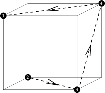
Figure 7:

Using the assignments eq. (8) one sees that a weak isospin transformation corresponds to reversing a permutation, i.e. reversing all 3 arrows in a figure like fig. 7. This way weak isospin is not any more a quantum number carried by a fundamental constituent but is determined by the binding of the state. Later on, a somewhat similar picture will be suggested for the understanding of electric and color charge of the first family. One can easily see that the assignments eqs. (7) and (8) are equivalent. One just has to project the closed path in fig. 8 on a square. In so doing the permutation $\overline{2341}$ corresponds to the rotation $C_{4}^{2}$ etc.

Figure 8: Closed path I in $S_{4}$. The endpoints of the dashed lines form a tetrad. The projection of this path on a square leads to the equivalence of eqs. (7) and (8).

Figure 9: closed path II

Figure 10: closed path III

For completeness let us write down the $S_{4}$–assignment of the second and third generation. They correspond to the various paths consisting of 3 links which one can draw into the closed loops depicted into figs. 9 and 10.

$$\nu_{\mu L} = \overline{2134}\qquad c^{1}_{L}=\overline{1342}\qquad c^{2}_{L}=\overline{3421}\qquad c^{3}_{L}=\overline{4213}$$

$$\mu_{L} = \overline{4312}\qquad s^{1}_{L}=\overline{2431}\qquad s^{2}_{L}=\overline{1243}\qquad s^{3}_{L}=\overline{3124}$$ (9)

$$\nu_{\tau L} = \overline{4231}\qquad t^{1}_{L}=\overline{2314}\qquad t^{2}_{L}=\overline{3142}\qquad t^{3}_{L}=\overline{1423}$$

$$\tau_{L} = \overline{1324}\qquad b^{1}_{L}=\overline{4132}\qquad b^{2}_{L}=\overline{2413}\qquad b^{3}_{L}=\overline{3241}$$ (10)

It should be noted that there is an intimate connection between the 3 closed paths figs. 8, 9 and 10 and the 3 planes in fig. 3, i.e. the dimensionality of space. Fig. 8 corresponds to the first family plane, Fig. 9 to the second family plane and Fig. 10 to the third family plane. This can be seen easily by drawing the octahedron with corners given by the middle points of the cube’s face diagonals.

Now for the question of electric and color charge. We want to adjoin quantum numbers to the various permutations above. There are several possibilities to solve this problem. As an example, we suggest the following construction. First of all, let us modify and refine the state identification given in eqs. (8–10) a little bit. Look at the four states

$$v_{1}=\overline{4321}\qquad v_{2}=\overline{1432}\qquad v_{3}=\overline{2143}\qquad v_{4}=\overline{3214}$$ (11)

which were preliminary identified as $e_{L}$, $d^{1}_{L}$, $d^{2}_{L}$ and $d^{3}_{L}$ in eq. (8). Consider them as an orthonormal basis of an artificial vector space, i.e. $v_{i}\cdot v_{j}=\delta_{ij}$. Instead of $v_{1}$ we want to identify the linear combination ${1\over 4}(v_{1}+v_{2}+v_{3}+v_{4})$ as the lefthanded electron $e_{L}$, and the quark states $d^{1}_{L}$, $d^{2}_{L}$ and $d^{3}_{L}$ should span the subspace orthogonal to this linear combination, i.e.

$$e_{L}={1\over 4}(v_{1}+v_{2}+v_{3}+v_{4})=(+++)_{v}$$ (12)

$$d^{1}_{L}={1\over 4}(v_{1}-v_{2}-v_{3}+v_{4})=(--+)_{v}$$ (13)

$$d^{2}_{L}={1\over 4}(v_{1}+v_{2}-v_{3}-v_{4})=(+--)_{v}$$ (14)

$$d^{3}_{L}={1\over 4}(v_{1}-v_{2}+v_{3}-v_{4})=(-+-)_{v}$$ (15)

where in the second part of these equations we have described the states by the relative sign of the coefficients of $v_{i}$ and $v_{1}$. Now we associate an additive quantum number $Q(+)_{v}=-{1\over 3}$ and $Q(-)_{v}=0$ to those signs in order to obtain $Q(e_{L})=-1$ and $Q(d_{L})=-{1\over 3}$.

A similar construction can be carried out for the states $\overline{1234}$, $\overline{2341}$, $\overline{3412}$ and $\overline{4123}$, from which one can form linear combinations ${1\over 4}(\overline{1234}+\overline{2341}+\overline{3412}+\overline{4123})\equiv(+++)_{w}$ etc. in the same way as eqs. (12–15). Note that this time the charge assignment should be $Q(-)_{w}=-{1\over 3}$ and $Q(+)_{w}=0$ in order to ensure $Q(\nu)=0$ and $Q(u)={2\over 3}$.

Now about the color charge: it is defined to operate on the three–dimensional space spanned by $d^{1}_{L}$, $d^{2}_{L}$ and $d^{3}_{L}$ (and similarly for the other quark flavors and helicities). A priori, the color degrees of freedom introduced here are purely real. However, one needs complex representations in order to accomodate antiparticles. One possibility is that one artificially complexifies the vector spave spaned by $d^{1}_{L}$, $d^{2}_{L}$ and $d^{3}_{L}$. I think this is acceptable in the present situation, in which the true meaning of forming those linear combinations is unclear. It has to do with the specific way the preons on the sites of the tetrads are bound.

Note that the construction presented here has a similarity to the charge assignment and the structure of the ’richon’ model [2]. The states T and V of the Rishon model correspond to the various ways in which the above linear combinations are formed, $T\sim(+)$ and $V\sim(-)$. This is, however, the only similarity to preon models of that type. Those were constructed with an eye on obtaining a decent field theory but have some very unsatisfactory features. For example, there is no understanding whatsoever of parity violation. Parity violation and vector bosons will be discussed in the next section.

In the literature there have been some attempts to use finite nonabelean groups to describe the family repetition structure. Usually, representations are considered to model the generations, and a complicated Higgs sector is constructed to account for the observed mass differences between the fermions. In my opinion, this does not really solve the mass problem but just shifts it to another level. It would be much more desirable to understand the fermion masses dynamically, in the model at hand, for example, by understanding the differences between the bindings of preons 1, 2, 3 and 4.

6. Vector Bosons

Now that we have constructed all states of the fermion generations the most important question is how to understand their interactions. As is well known the interactions of fermions proceed through left– and right–handed currents with the vector bosons, more precisely the lefthanded currents $\bar{F}_{L}\times f_{L}$ : $=\bar{F}_{L}\gamma_{\mu}f_{L}$ interact with the weak bosons and the sum of left- and righthanded currents interact with photons and gluons. The strength of the photonic and gluonic interaction is given by the electric and color charge, respectively.

The picture to be developed is that of the vector bosons as a sort of fermion–antifermion bound state. However, it will be constructed in such a way that the vector bosons do not ’remember’ the flavor of the fermion–antifermion pair from which they were originally formed. The way to obtain antiparticles (and Dirac fermions) is as follows: I have already shown that left– and right–handed fields are interpreted as permutations of corners 1,2,3,4 and 1’,2’,3’,4’ in the cube (cf. fig. 11), for example $e_{L}=\overline{4321}$ and $e_{R}=\overline{4^{\prime}3^{\prime}2^{\prime}1^{\prime}}$. The antiparticle of a lefthanded fermion is a righthanded object and its preons should form a righthanded tetrad. Therefore, the $\bar{e}_{L}$ is defined to live on the righthanded tetrad ($\overline{4^{\prime}3^{\prime}2^{\prime}1^{\prime}}$) but with field values corresponding to the complex conjugate of $e_{L}$. Similarly $\bar{e}_{R}=\overline{4321}$, with field values which are complex conjugate to $e_{R}$. Antifield configurations are denoted by open circles in fig. 11. More precisely, the combinations of a lefthanded fermion of the first family and their righthanded antiparticles are shown in fig. 11. This way all the corners of the cube are filled. Fig. 11 more or less represents how vector bosons should be imagined in this model.

Figure 11: A vector boson from fermion (full circle) and antifermion (open circle). It forms a closed loop in the first family plane.

Fig. 11 is a rather characteristic picture of a fermion–antifermion bound state. The point is that the vector boson interactions always take place within one family, and fig. 11 corresponds to interactions within the first family. One sees that the bindings between the links join together to form bindings along the plaquettes. Altogether, the bindings form an oriented closed circle of plaquettes. In the case of the second family interactions there is also a closed circle and it lies in the second family plane (cf. fig. 3) and similarly for interactions between members of the third family. The three planes can be rotated into each other to make the corresponding vector bosons identical. The difference to fermions will be understood better in a group representation approach to be discussed below.

In my model, vector bosons are superpositions of fermion–antifermion states $\bar{F}\times f$ with the appropriate quantum numbers. The $\bar{F}\times f$ binding arises from interactions along the four body diagonals of the cube defined by fermions (1234) and antifermions (1’2’3’4’), i.e. interactions between the full and open circles in fig. 11. I shall come back to the body diagonals later.

	$I$	$8C_{3}$	$3C_{4}^{2}$	$6C_{2}$	$6C_{4}$
	Photon	Gluons	$W_{1,2,3}$	Leptoquarks X	Leptoquarks Y
$A_{1}$($U(1)_{Y}$)	1	1	1	1	1
$A_{2}$	1	1	1	-1	-1
$E$ ($SU(2)_{L}$)	2	-1	2	0	0
$T_{1}$	3	0	-1	1	-1
$T_{2}$($SU(3)_{c}$)	3	0	-1	-1	1

Table 1: Character Table of $S_{4}$ and corresponding $SU(5)$ assignments. The form of the representation spaces are reminiscent of the $U(1)\times SU(2)_{L}\times SU(3)$ breaking structure from $SU(5)$.

For finite groups the number of irreducible representations (IR’s) is equal to the number of conjugacy classes. In the present case the IR’s are usually called $A_{1}$, $A_{2}$, $E$, $T_{1}$ and $T_{2}$ with dimensions 1, 1, 2, 3 and 3, respectively, and their characters are shown in table 1. $A_{1}$ is the identity representation. $A_{2}$ differs from $A_{1}$ by having a negative value for odd permutations. $T_{1}$ is the representation induced by the permutations of the corner points 1,2,3,4 of a tetrad in three dimensions. Its representation space is therefore the three dimensional space, in which the fermions live, i.e. $T_{1}$ konstituiert den Anschauungsraum. $T_{2}$ is obtained from $T_{1}$ by changing the sign of the representation matrices for the odd permutations. Finally, $E$ is induced by a representation of $S_{3}$ on the corners of a triangle, as discussed at the end of section 4 and fig. 4, for example $E(\overline{2134})\bf{a}=\bf{b}$, $E(\overline{2134})\bf{b}=\bf{a}$, $E(\overline{2134})\bf{c}=\bf{c}=-\bf{a}-\bf{b}$, $E(\overline{1243})\bf{a}=\bf{b}$, $E(\overline{1243})\bf{b}=\bf{a}$, $E(\overline{1243})\bf{c}=\bf{c}=-\bf{a}-\bf{b}$, etc [1].

In order to obtain the vector bosons $\bar{F}\times f$, one should take the 9–dimensional product representation

$$T_{1}\times T_{1}=A_{1}+E+T_{1}+T_{2}$$ (16)

On the right hand side, the term $T_{1}$ corresponds to arbitrary rotations of the closed loops of plaquettes, as claimed in connection with fig. 11. $A_{1}$ corresponds to the photon, the totally symmetric singlet configuration, where all tetrad–antitetrad combinations contribute in the same way. $T_{2}$ is induced by 24 permutations of some objects I,II,III,IV (much like the $T_{1}$ on the left hand side of equation (16) was induced by the 24 permutations of 1,2,3,4). Finally, $E$ is induced by the 6 permutations on the triangle (fig. 4).

A possible interpretation of $T_{2}$ is as follows : By definition, the different vector bosons correspond to permutations of the cube’s four body diagonals called I, II , III and IV, which define another group $S_{4}$. It is ordered not as in the case of fermions, equations (8)–(10), but according to its conjugacy classes. In fact, the 24 elements of $S_{4}$ can be ordered in 5 conjugacy classes with 1, 3, 8, 6 and 6 elements. They are given as follows:

• identity
  $\overline{I,II,III,IV}$
  the U(1) gauge boson

• 3 $C_{2}$ rotations by $\pi$ about the coordinates axes x, y and z
  $\overline{II,I,IV,III}$,   $\overline{III,IV,I,II}$,   $\overline{IV,III,II,I}$
  the SU(2) gauge bosons

• 8 $C_{3}$ rotations by $\pm{2\over 3}\pi$ about the cube diagonals (like x=y=z)
  $\overline{II,III,I,IV}$,   $\overline{III,I,II,IV}$,   $\overline{II,IV,III,I}$,   $\overline{IV,I,III,II}$,
  $\overline{III,II,IV,I}$,   $\overline{IV,II,I,III}$,   $\overline{I,III,IV,II}$,   $\overline{I,IV,II,III}$
  the gluons

• 6 $C_{4}$ rotations by $\pm{\pi\over 2}$ about the coordinate axes
  $\overline{II,I,III,IV}$,   $\overline{III,II,I,IV}$,   $\overline{IV,II,III,I}$,
  $\overline{I,III,II,IV}$,   $\overline{I,IV,III,II}$,   $\overline{I,II,IV,III}$
  leptoquarks

• 6 $C_{2}^{\prime}$ rotations by $\pi$ about axes parallel to the face diagonals (like x=y, z=0)
  $\overline{II,III,IV,I}$,   $\overline{II,IV,I,III}$,   $\overline{III,IV,II,I}$,
  $\overline{III,I,IV,II}$,   $\overline{IV,III,I,II}$,   $\overline{IV,I,II,III}$
  leptoquarks

where reference is made to the cartesian coordinates x,y and z with origin at the cube’s centre. This ordering is reminiscent of the ordering of gauge bosons in grand unified theories where there are leptoquarks in addition to the 8 gluons and the four electroweak gauge fields. The elements of the first two classes form Klein’s 4–group (an abelean subgroup of $S_{4}$), whereas the elements of the first three classes form the nonabelean group of even permutations.

In summary, the interpretation of eq. (16) is as follows: As discussed before, the fermions constitute ordinary three–dimensional space. As soon as two fermions approach each other to form a vector boson, space opens up to 9 dimensions. Three of them correspond to ordinary space, whereas the remaining six decompose into 1+2+3 dimensional representation spaces $A_{1}$, $E$ and $T_{2}$ of $S_{4}$. They become fibers to ordinary space. It remains to be shown how the complex structure of a $U(1)\times SU(2)\times SU(3)$ Lie algebra arises.

Since parity violation is not present in these pictures, I want to add an alternative related to the observation that there are two 1–dimensional and two 3–dimensional, but only one 2–dimensional IR of $S_{4}$. One could relate parity transformations to even–odd transitions between permutations by modifying the assignments made in equations (8)–(10), namely

$$\nu_{L} = \overline{1234}\qquad u^{1}_{R}=\overline{2341}\qquad u^{2}_{L}=\overline{3412}\qquad u^{3}_{R}=\overline{4123}$$

$$e_{L} = \overline{4321}\qquad d^{1}_{R}=\overline{1432}\qquad d^{2}_{L}=\overline{2143}\qquad d^{3}_{R}=\overline{3214}$$ (17)

i.e. assigning odd permutations to righthanded states. According to the character table 1 the character of $E$ vanishes for odd permutations. Therefore, there is no action of $E$ on righthanded fermions. In contrast, the products $A_{1}\times A_{2}$ and $T_{1}\times T_{2}$ act like $-\gamma_{5}$ on left and righthanded fermions.

8. Conclusions

According to present ideas the elementary particles (leptons, quarks and vector bosons) are pointlike and their mathematical description follows this philosophy (Dirac theory, Yang–Mills theory). They certainly receive an effective extension by means of quantum effects, but these are fluctuations and do not affect the primary idea of pointlike objects.

In contrast, in the preon picture the observed fermions naturally have an extension right from the beginning. This seems to be difficult to accomodate because their radius should be of the order of their inverse masses. Following t’Hooft one may assume that there is a symmetry principle which leaves the masses small.

The models in this paper do not allow to make quantitative predictions of fermion masses. Some qualitative statements about fermion masses can be found in sections 2 and 3. As compared to the binding energy, all fermion masses (including $m_{t}$) are tiny perturbations which might be induced by some radiative mechanism of the ’effective’ standard model interactions leading to masses $\sim\alpha^{F}$ for the F–th family. The ’textures’ of those masses have been discussed in section 2 (cf. [4] for more elaborate approaches).

Within the models of sections 4, 5 and 6 one may assume that the fermions are basically massless by some symmetry and that there are small symmetry breaking effects within the family planes leading to different family masses eq. 2.

Whatever this symmetry principle may be, there is still the question how large the radius R of the quarks and leptons is. In principle, there are three possibilities, it may be large ($\sim 1$ TeV^-1), small ($\sim M_{Planck}^{-1}$) or somewhere in between. In the first case there will be experimental signals for compositeness very soon. In the second case there will never be direct experimental indications and it will be difficult to verify the preon idea. Furthermore, in that case one would have the GUT theories as correct effective theories whose particle content would have to be explained. In addition, it may be necessary to modify the theory of relativity. In fact, the superstring models are a realization of this idea, the ’preons’ being strings instead of point particles.

Personally, I like the scenario $R\sim M_{Planck}^{-1}$ reasonably well. In the model presented in this paper, the preons are pointlike and sitting on a cubic lattice. This lattice would have to fluctuate in some sense to reconstitute Lorentz invariance. This certainly raises many questions which go beyond the scope of this article. For example, the renormalization of gravity would be modified because high energies ($>M_{Planck}$) would be cut away by the lattice spacing.

As for the third possibility 1 TeV $<<R<<M_{Planck}$, gravity and its problems play no role and my models are just a more or less consistent picture of particle physics phenomena. Since no attempt was made to explicitly construct the states of quarks and leptons in their known complex representations they are at best a qualitative guideline for understanding. I did not write a Lagrangian for the preons and just speculated about their interactions. The ultimate aim would be to construct a Lagrangian and derive from it an effective interaction between Dirac fermions and gauge fields.

Acknowledgements

With this paper my scientific efforts come to an end. After 18 years of hard work I have not been able to find a reasonable position in physics.

References

-
[1]
W.L. van der Waerden, Algebra I and II, Springer Verlag
R.C. Johnson, Phys. Lett. 114B (1982) 147 - [2] H. Harari and N. Seiberg, Nucl. Phys. B204 (1982) 141
- [3] G. t’Hooft, Proc. Cargese Summer Inst., 1979.
- [4] P. Ramond, R.G. Roberts and G.G. Ross, Nucl. Phys. B406 (1993) 19