Current Status of the Resonant Spin-Flavor Precession Solution to the Solar Neutrino Problem

Abstract

We discuss the current status of the resonant spin-flavor precession (RSFP) solution to the solar neutrino problem. We perform a fit to all the latest solar neutrino data for various assumed magnetic field profiles in the Sun. We show that the RSFP can account for all the solar neutrino experiments, giving as good fit as other alternative solutions such as MSW or vacuum oscillation (Just So), and therefore can be a viable solution to the solar neutrino problem

I Introduction

The solar neutrino anomaly has been more and more strongly established both in its experimental [1, 2, 3, 4, 5] as well as in its theoretical [6, 7, 8, 9] aspect. In fact, both have presented a very dynamical evolution. From one side, theoretical predictions, i.e., the standard solar models (SSM), have been refined by including several mechanisms such as helium diffusion [7, 8] and an updating analysis of the $S_{17}$ astrophysical factor [8, 10]. One can see in ref. [11] that theoretical predictions obtained by different SSMs, which are developed independently, are in good agreement with each other. Moreover, it has been shown that the SSM is in excellent agreement with the helioseismology [8].

On the other hand, experimental data have become more accurate due to the calibration of the experiments, more statistics and the existence of the new generation SuperKamiokande experiment and its solar neutrino spectral observations [5]. Consequently, final numbers related to the solar neutrino deficit have also evolved significantly. The most updated experimental data as well as theoretical predictions are shown in Table I. One can show that these observed solar neutrino data are in strong disagreement with the ones predicted by the SSM [11, 12]. Moreover, this conclusion does not depend on any details of the SSM.

Solutions to the solar neutrino problem rely on different phenomena  [13] which deplete the number of observable neutrinos at the Earth: neutrino oscillations in vacuum [14], resonantly enhanced matter oscillations [15], resonant spin-flavor precession phenomenon (RSFP) [16, 17] and flavor mixing by new interactions [18, 19]. The capability of each one of these processes to make compatible solar neutrino predictions and observations and therefore to find a solution to the solar neutrino anomaly have been updated from time to time [20]. In this paper we investigate the current status of the RSFP scenario [21]. We believe that it is worthwhile to reanalyse this mechanism in the light of new solar neutrino data as well as the new SSM. We also discuss briefly how the solar neutrino spectral observations in SuperKamiokande are affected by the RSFP mechanism.

TABLE I.: Observed solar neutrino event rates used in this analysis and corresponding predictions from the reference standard solar model [8]. The quoted errors are at $1\sigma$.

Experiment	Data $\pm$(stat.) $\pm$(syst.)	Ref.	Theory [8]	Units
Homestake	$2.56\pm 0.16\pm 0.15$	[1]	$7.7^{+1.2}_{-1.0}$	SNU
SAGE	$69.9^{+8.0}_{-7.7}{}^{+3.9}_{-4.1}$	[3]	$129^{+8}_{-6}$	SNU
GALLEX	$76.4\pm 6.3^{+4.5}_{-4.9}$	[4]	$129^{+8}_{-6}$	SNU
SuperKamiokande	$2.44\pm+0.05{}^{+0.09}_{-0.06}$	[5]	$5.15^{+0.98}_{-0.72}$	$10^{6}$ cm-2s-1

RSFP mechanism is very sensitive to the magnetic profile in the Sun and, in fact, several possible scenarios for the magnetic strength have been proposed by different authors [22, 23, 24, 25, 26]. We consider several possibilities which include the main qualitative aspects of the magnetic profile in the Sun previously invoked as a solution to the solar neutrino anomaly. Using the minimum $\chi^{2}$ method to compare theoretical predictions of the RSFP phenomenon and the experimental observations we conclude that very good fits can be obtained for the average solar neutrino suppression, if intense magnetic fields in the solar convective zone are considered.

II RSFP mechanism

Assuming a nonvanishing transition magnetic moment of neutrinos, active solar neutrinos interacting with the magnetic field in the Sun can be spin-flavor converted into sterile nonelectron neutrinos [27, 28] (if we are dealing with Dirac particles) or into active nonelectron antineutrinos [29] (if the involved particles are Majorana). In both cases the resulting particles interact with solar neutrino detectors significantly less than the original active electron neutrinos in such a way that this phenomenon can induce a depletion in the detectable solar neutrino flux.

Spin-flavor precession of neutrinos can be resonantly enhanced in matter [16, 17], in close analogy with the MSW effect [15]. In this case the precession strongly depends on the neutrino energy and provokes different suppressions for each portion of the solar neutrino energy spectrum. Therefore RSFP provides a satisfactory description [21, 22, 23, 24, 25, 26] of the actual experimental panorama [1, 2, 3, 4, 5]: all experiments detect less than the theoretically predicted solar neutrino fluxes [8] and different suppressions are observed in each experiment, suggesting that the mechanism to conciliate theoretical predictions and observations has to differentiate the different parts of the solar neutrino spectrum.

For simplicity, we consider two generation of neutrinos, electron neutrino and, for e.g., muon neutrino (which could be replaced by tau neutrino in our discussion). Furthermore, we assume that the vacuum mixing angle is zero or small enough to be neglected. (See ref. [30] for the case where RSFP and flavor mixing simultaneously exists.) The time evolution of neutrinos interacting with a magnetic field $B$ through a nonvanishing neutrino magnetic moment $\mu_{\nu}$ in matter is governed by a Schrödinger-like equation [16, 17];

$$i\frac{d}{dt}\left(\begin{array}[]{l}\nu_{e_{L}}\\ \overline{\nu}_{\mu_{R}}\end{array}\right)=\left(\begin{array}[]{cl}a_{\nu_{e}}&\mu_{\nu}B\\ \mu_{\nu}B&\frac{\Delta m^{2}}{2E}+a_{\nu_{\mu}}\end{array}\right)\left(\begin{array}[]{l}\nu_{e_{L}}\\ \overline{\nu}_{\mu_{R}}\end{array}\right),$$ (1)

where $\nu_{e}$ and $\overline{\nu}_{\mu_{R}}$ are active electron neutrinos and muon antineutrinos, respectively, $\Delta m^{2}=m^{2}_{\nu_{\mu}}-m^{2}_{\nu_{e}}$ is their squared mass difference and $E$ is the neutrino energy, $a_{\nu_{e}}=G_{F}(2N_{e}-N_{n})/\sqrt{2}$ and $a_{\nu_{\mu}}=G_{F}N_{n}/\sqrt{2}$, with $N_{e}$ and $N_{n}$ being electron and neutron number densities, respectively. In eq. (1) we are assuming that neutrinos are Majorana particles. For the Dirac case, the spin-flavor precession involves $\nu_{e}\leftrightarrow\nu_{s}$, where $\nu_{s}$ is a sterile neutrino and $a_{\nu_{s}}=0$.

FIG. 1.: Matter potentials as a function of radial distance from the solar center are plotted. The solid and dotted curves correspond to the Majorana and Dirac case, respectively. The dashed line correspond to $\mu_{\nu}B=10^{-11}\mu_{B}\times 100$ kG.

III Analysis

In order to obtain the survival probability we first numerically integrate the evolution equations (1) varying matter density in the Sun [6] for some assumed profiles of the magnetic field which will be described below. Next, using the solar neutrino flux in ref. [8], we compute the expected solar neutrino event rate in each experiment, taking into account the relevant absorption cross sections [6] for ⁷¹Ga  and ³⁷Cl experiments as well as the scattering cross sections for $\nu_{e}$-$e^{-}$ and $\bar{\nu}_{\mu}$-$e^{-}$ reactions including also the efficiency function for the SuperKamiokande experiment in the same way as in ref. [31]. We note that in this analysis we always adopt the solar model in ref. [8] as a reference SSM.

FIG. 2.: Various magnetic field profiles used in this work. For each field $\langle B\rangle$ is defined as the average of the field over the region where $B(r)$ is not zero.

A Assumptions

We do not take into account the production point distribution of neutrinos. This can be justified by two main reasons. For the relevant values of $\Delta m^{2}$ our analysis shows that (see below) the resonance position lyes always outside the neutrino production region ($r/R_{\rm SUN}<0.3$) because the solutions we find implies $\Delta m^{2}\raise 1.29167pt\hbox{$\;<$\kern-7.5pt\raise-4.73611pt\hbox{$\sim\;$}}10^{-7}$ eV². In order to see this we plot in Fig. 1 the matter potential as a function of the radial distance from the solar center.

If neutrinos are considered Majorana particles, $V_{\rm matter}\equiv a_{\nu_{e}}-a_{\nu_{\mu}}$, and if they are Dirac, $V_{\rm matter}\equiv a_{\nu_{e}}$. It is shown, in the right ordinate in the same plot, also the value of the quantity $\Delta m^{2}$ to which a resonance is found. For example, if $\Delta m^{2}=10^{-7}$ eV² (for $E$= 1 MeV), a resonance is localized in $r/R_{\rm SUN}\approx 0.52$. Therefore, it can be seen that the resonance position is also larger than $r/R_{\rm SUN}=0.3$, outside the production region. Also, the range of $\mu_{\nu}B$ we consider here is much smaller than the matter potential, $a_{\nu_{e}}$ and $a_{\nu_{\mu}}$, in the production region. Again this fact is shown in Fig. 1, where the quantity $\mu_{\nu}B=10^{-11}\mu_{B}\times 100$ kG is presented. Therefore, from eq. (1) we observe that neutrino spin-flavor precession is prevented before neutrino gets the resonance region and the final survival probability is not affected by the production position.

It is obvious from the evolution equations (1) that the RSFP mechanism crucially depends on the solar magnetic field profile along the neutrino trajectory. In the present paper we choose several different profiles which, we believe, cover in general all the previously [22, 23, 24, 25, 26] analysed magnetic profiles which led to a solution to the solar neutrino anomaly. In Fig. 2, these magnetic fields are presented in their general aspects. The constant magnetic profile $B_{1}(r)$ was adopted in references [24], while the general aspects of the profiles $B_{3}(r)$ and $B_{4}(r)$ have already appeared in refs. [23, 25, 22], and [26], respectively. We note that close to the solar surface ($r>0.95R_{\odot}$) we have switched off the magnetic field for all the profiles we considered in this work.

B Definition of $\chi^{2}$

The relevant free parameters in the RSFP mechanism are $\Delta m^{2}$ and $\mu_{\nu}B$. Using the solar neutrino data given in Table I, we look for the region in the $\Delta m^{2}-\mu_{\nu}\langle B\rangle$ parameter space, where $\langle B\rangle$ denotes the average field strength defined as in Fig. 2, which leads to a solution to the solar neutrino anomaly by means of the minimum $\chi^{2}$ method. In this analysis we will use only the SuperKamiokande data [5] without including the Kamiokande data [2] because of the larger statistics and the smaller systematic error in the SuperKamiokande experiment. We also note that we will use the combined value of the two ⁷¹Ga  experiments, 72.3 $\pm$ 5.6 SNU.

Our $\chi^{2}$ is defined as follows,

$$\chi^{2}=\sum_{i,j}(R_{i}^{th}-R_{i}^{obs})[\sigma^{2}_{ij}(\mbox{tot})]^{-1}(R_{j}^{th}-R_{j}^{obs}),$$ (2)

where $(i,j)$ run through three experiments, i.e., ⁷¹Ga  , ³⁷Cl and SuperKamiokande, and the total error matrix $\sigma^{2}_{ij}(\mbox{tot})$ and the expected event rates $R_{i}$ are computed as follows. We essentially follow ref. [32] for the derivation of the error matrix and to describe the correlations of errors we used in this work. The expected experimental rates in the absence of neutrino conversion is given by,

$$R_{i}=\sum_{j}C_{ij}\phi_{j}\ \ \ (i=\mbox{Ga},\ \mbox{Cl},\ \mbox{SK}),$$ (3)

where $C_{ij}$ is the cross section coefficients and $\phi_{j}$ is the solar neutrino flux. In Sec. IV where we consider the case with neutrino conversion we use the coefficients $C_{ij}$ determined by properly convoluting the conversion probability in the integration over the neutrino energy spectrum for each detector and neutrino flux. In this work we consider neutrino from $pp$, $pep$, ⁷Be, ⁸B, ¹³N and ¹⁵O sources and neglect other minor flux such as ¹⁷F and $hep$ neutrinos.

The total error matrix $\sigma^{2}_{ij}$ is the sum of the theoretical $\sigma^{2}_{ij}(\mbox{th})$ and experimental one $\sigma^{2}_{ij}(\mbox{exp})$,

$$\sigma^{2}_{ij}(\mbox{tot})=\sigma^{2}_{ij}(\mbox{th})+\sigma^{2}_{ij}(\mbox{exp}).$$ (4)

The theoretical error matrix can be further divided into the one coming from the uncertainties in the cross sections, $\sigma^{2}_{ij}(\mbox{cross})$ and the one coming from uncertainties in the solar neutrino flux, $\sigma^{2}_{ij}(\mbox{flux})$,

$$\sigma^{2}_{ij}(\mbox{th})=\sigma^{2}_{ij}(\mbox{cross})+\sigma^{2}_{ij}(\mbox{flux}).$$ (5)

The cross section error matrix $\sigma^{2}_{ij}(\mbox{cross})$ can be calculated by,

$$\sigma^{2}_{ij}(\mbox{cross}) = \delta_{ij}\sum_{k,l=1}^{6}\frac{\partial R_{i}}{\partial\mbox{ln}C_{kj}}\frac{\partial R_{j}}{\partial\mbox{ln}C_{lj}}\Delta\mbox{ln}C_{kj}\Delta\mbox{ln}C_{lj}$$ (6)

$$= \delta_{ij}\sum_{k=1}^{6}(R_{ik}\Delta\mbox{ln}C_{ik})^{2},$$ (7)

where $R_{ik}\equiv C_{ik}\phi_{k}$.

On the other hand, the flux error matrix $\sigma^{2}_{ij}(\mbox{flux})$ can be calculated by,

$$\sigma^{2}_{ij}(\mbox{flux}) = \sum_{k,l=1}^{6}\frac{\partial R_{i}}{\partial\mbox{ln}\phi_{k}}\frac{\partial R_{j}}{\partial\mbox{ln}\phi_{l}}\sum_{m=1}^{11}(\Delta\mbox{ln}\phi_{k})_{m}(\Delta\mbox{ln}\phi_{l})_{m}$$ (8)

$$= \sum_{k,l=1}^{6}R_{ik}R_{jl}\sum_{m=1}^{11}(\Delta\mbox{ln}\phi_{k})_{m}(\Delta\mbox{ln}\phi_{l})_{m},$$ (9)

where $(\Delta\mbox{ln}\phi_{k})_{m}$ is the fractional uncertainty of the $k$-th neutrino flux coming from the uncertainty in the $m$-th input parameter ($S_{11}$, $S_{33}$, $S_{34}$, $S_{17}$, $Z/X$, opacities, $S_{1,14}$, luminosity, age, diffusion or ⁷Be + $e^{-}$ capture rate) which are obtained by the computer code exportrates.f, available at URL http://www.sns.ias.edu/^∼jnb/. We note that in eq. (8) the product $(\Delta\mbox{ln}\phi_{k})_{m}(\Delta\mbox{ln}\phi_{l})_{m}$ takes positive (negative) value when $k$-th and $l$-th fluxes are positively (negatively) correlated to each other with respect to the variation of the $m$-th input parameter.

The experimental error matrix is given by,

$$\sigma^{2}_{ij}(\mbox{exp})=\delta_{ij}\sigma_{i}\sigma_{j},$$ (10)

where $\sigma_{i,j}$ ($i,j$ = Ga, Cl, SK) stands for the combined error in each experiment.

In Table II we show the correlation matrix $\rho_{ij}$ defined as,

$$\rho_{ij}\equiv\frac{\sigma^{2}_{ij}(\mbox{tot})}{\sqrt{\sigma^{2}_{ii}(\mbox{tot})\ \sigma^{2}_{jj}(\mbox{tot})}}.$$ (11)

TABLE II.: The correlation matrix $\rho_{ij}$ obtained from eqs. (4)-(11).

Experiment	Correlation matrix
Ga	1.00
Cl	0.497	1.00
Super-Kam	0.486	0.952	1.00

FIG. 3.: The contour plots of the survival probability in the $\langle B\rangle-\Delta m^{2}/E$ plane are shown in (a), (b), (c) and (d) for the magnetic field profiles, $B_{1}$, $B_{2}$, $B_{3}$ and $B_{4}$, respectively, sketched in Fig. 2.

IV Results

Now we compute the spin-flavor conversion probability, by numerically integrating the evolution eq. (1), assuming $\mu_{\nu}=10^{-11}\mu_{B}$ as a reference value, which is slightly below the present experimental upper bound [33]. Hereafter we always assume this value of magnetic moment [34] in this work but as it is clear from eq. (1) if $\mu_{\nu}$ is assumed to be smaller by certain amount, the same effect can still be obtained by simply increasing the value of magnetic field strength properly so that the product $\mu_{\nu}B$ would not be changed.

In Fig. 3 (a), (b), (c) and (d) we show the contour plots of the survival probability $P(\nu_{e}\to\nu_{e})=|\langle\nu_{e}(t)|\nu_{e}(0)\rangle|^{2}$ in the $\Delta m^{2}-\langle B\rangle$ parameter space, for the magnetic profiles we sketched in Fig. 2, $B_{1}(r)$, $B_{2}(r)$, $B_{3}(r)$ and $B_{4}(r)$, respectively. We note that the field $B_{3}$ gives very different probability contours from the other profiles, which will be also reflected in the final allowed region (see below).

Including now the experimental observations on the solar neutrino signal above shown in Table I, we can determine the region in the $\Delta m^{2}-\langle B\rangle$ parameter space which leads to a RSFP solution to the solar neutrino problem for a specified confidence level. We present the $\Delta m^{2}-\langle B\rangle$ parameter region which can account for all the solar neutrino data, at 90, 95 and 99 % C. L. in Figs. 4 (a), (b), (c) and (d), for the magnetic profiles $B_{1}(r)$, $B_{2}(r)$, $B_{3}(r)$ and $B_{4}(r)$, respectively.

We observe from Figs. 4 (a) to (d) that a solution to the solar neutrino problem can be found when $\langle B\rangle\raise 1.29167pt\hbox{$\;>$\kern-7.5pt\raise-4.73611pt\hbox{$\sim\;$}}$ few times 10 kG and $\Delta m^{2}$ is the order of $10^{-8}$ to $10^{-7}$ eV² for any of the magnetic profiles used in this work. Nevertheless, the quality of the fit, measured by the minimum $\chi^{2}$ criterion, varies a lot. The poorest fit is obtained when the continuously decaying magnetic field profile $B_{4}$ is used, with $\chi^{2}_{min}=6.1$ for one (three data points - two free parameters) degrees of freedom. Better fits are obtained when the $B_{1}$ (uniform) and $B_{2}$ (large triangle) fields are employed showing $\chi^{2}_{min}=2.0$ and 1.8, respectively. And the best fit appears when the triangular field in the solar convective zone, $B_{3}$, is employed, with a rather small value $\chi^{2}_{min}=0.13$. For this profile, we note that, as expected from Fig. 3 (c) we have several local best fit points also indicated in Fig. 4 (c) by the open circles whose corresponding $\chi^{2}_{min}$ are, from left to right, 2.3, 0.29 and 0.19.

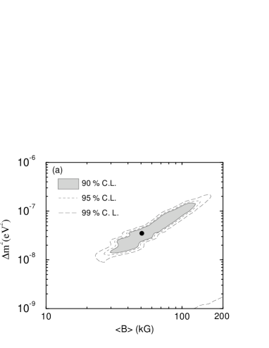
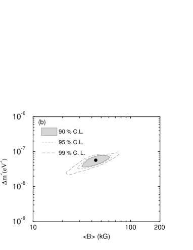
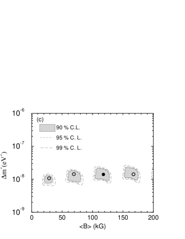
FIG. 4.: The Allowed RSFP solution to the solar neutrino problem. The parameter region allowed at 90, 95 and 99 % C. L. are shown in (a), (b), (c) and (d) for the magnetic field profiles, $B_{1}$, $B_{2}$, $B_{3}$ and $B_{4}$, respectively, sketched in Fig. 1. We indicate best fit points by filled circles. In (c) we also indicate, by the open circles, the local best fit points inside each island delimited by 90 % C.L. curves.

The reason why we are getting very good fit for $B_{3}$ is that this profile can provide the required suppression patterns of various neutrino flux implied by latest the data [12] as discussed in ref. [25]. First we note that low energy $pp$ neutrinos are not so suppressed because the resonance positions are located in the inner region where the magnetic field is zero or small (see Figs. 1 and 2). However, intermediate energy ⁷Be neutrinos can be strongly suppressed due to the rapid increase of the field at the bottom of the convective zone since their resonance position is in a slightly outer region than the $pp$ one. On the other hand, high energy ⁸B neutrinos are moderately suppressed because their resonance positions are closer to the solar surface than the ⁷Be ones, where the field is decreasing. The best fitted values of $\langle B\rangle$ and $\Delta m^{2}$ as well as $\chi^{2}_{min}$ obtained from these different profiles are summarized in Table III.

TABLE III.: The best fitted parameters and $\chi^{2}_{min}$ for the Majorana case. Dirac case is presented in the parentheses.

Profile	$\langle B\rangle$ (kG)	$\Delta m^{2}$ (10-8 eV2)	$\chi^{2}_{min}$
1	50.6 (40.9)	3.5 (2.3)	2.0 (6.2)
2	47.1 (40.8)	6.1 (4.6)	1.8 (5.7)
3	118 (69.4)	1.5 (1.2)	0.13 (1.3)
4	82.9 (81.6)	8.1 (6.6)	6.1 (11.4)

We have repeated the same analysis also for the Dirac neutrino case. We, however, do not show the plots for the allowed region since they are rather similar to what have been presented above, if the same magnetic field profile is assumed. Instead, for the case of Dirac neutrinos, we only present the best fitted parameters and $\chi^{2}_{min}$ in the parentheses in Table III.

We see from this table that, the Dirac case always leads to a worse fit if the same magnetic field profile is assumed. To understand this we should note that for the Dirac case, $\nu_{e}$’s are converted into the right handed muon (or tau) neutrino, which do not contribute to any of the solar experiments including the water Chrenkov experiment [37]. In contrast in the Majorana case, converted right handed neutrino $\bar{\nu}_{\mu}$’s do contribute to the signal observed in the SuperKamiokande detector. This makes it difficult to conciliate the difference between the SuperKamiokande and ³⁷Cl data.

Let us now comment about the possibility of having such strong magnetic field in the Sun. While there is no generally accepted theory of solar magnetic field, it is possible to bound the field strength from very general arguments. It can be shown [6] that the magnetic field less than 10⁶ kG in the solar core or less than 10⁴ kG in the solar convective zone, will hardly affect the thermal structure and nuclear reaction processes well described by the standard solar model. These values come from the requirement that the magnetic pressure should be much smaller than the gas pressure, and can be regarded as the most generous upper limits of the magnetic field inside the Sun. More stringent bounds on the magnetic field in the convective zone are found in refs. [35, 36] where the discussion is based on the non-linear effects which eventually prevents the growth of magnetic fields created by the dynamo process. Naive limit can be obtained by estimating the required field tension necessary to prevent a fluid element from sinking into a magnetically stratified region, so that the magnetic flux would not be further amplified. By equating the magnetic tension to the energy excess of a sinking element at the bottom of the convective zone, Schmitt and Rosner [35] obtained $\sim 10$ kG as an upper bound for the magnetic field, which is of the order of the magnitude we need to have a good fit to the solar data by RSFP mechanism for the reference value of magnetic moment, $\mu_{\nu}=10^{-11}$ $\mu_{B}$.

Finally, we briefly discuss how the recoil electron energy spectra in the SuperKamiokande detector will be affected by the RSFP mechanism [38]. In Fig. 5 (a) we plot the electron neutrino survival probabilities as a function of neutrino energy using the best fit parameters. In Fig. 5 (b) we plot the recoil electron energy spectra divided by the standard prediction expected to be observed in the SuperKamiokande detector, using also the best fit parameters as in Fig. 5 (a). In Fig. 5 (b) we also plot the latest data from SuperKamiokande [5]. As we can see from the plot the observed data indicate some distortion mainly due to the last three data points in the higher energy bins. We, however, note from this plot that it seems difficult to exclude, at this moment, any of our predicted spectra expected from different field profiles, because of the experimental errors. We have to wait for more statistics and more careful analysis from the experimental group before drawing any definite conclusion.

FIG. 5.: We plot in (a) electron neutrino survival probability as a function of energy with the best fitted parameters for various field profiles. In (b) we plot recoil electron energy spectra expected from RSFP scenario using our best fit parameters, divided by the SSM prediction. The SuperKamiokande data are also shown by the filled circles with error bars. The last data point includes the contribution from the electrons with energy larger than 14 MeV.

V Conclusions

We have reanalysed the RSFP mechanism as a solution to the solar neutrino problem in the light of the latest experimental data as well as the theoretical predictions.

We found that the quality of the RSFP solution to the solar neutrino anomaly crucially depends on the solar magnetic field configuration along the neutrino trajectory inside the Sun. We found that the best fit to the observed solar neutrino data, which seems to be even better than the usual MSW solution as far as the total rates are concerned, is obtained if intensive magnetic fiels in the convective zone is assumed, in agreement with the conclusion found in ref. [25], whereas the linearly decaying magnetic field gives the worst fit. We, however, note that the required magnitude of the free parameters involved in the process, i.e., the magnetic field strength multiplied by the neutrino magnetic moment $\mu_{\nu}\langle B\rangle$ and the squared mass difference $\Delta m^{2}$, points to the same order, $\mu_{\nu}\langle B\rangle\approx\mbox{few\ times\ }10^{-11}\mu_{B}\cdot 10$ kG and $\Delta m^{2}\approx$ few times $10^{-8}$ eV², for any of the field profiles assumed in this work.

Our ignorance about the profile as well as the magnitude of the solar magnetic field makes this approach to the solar neutrino observation less predictive than its alternative approaches [14, 15, 18]. Nevertheless the presence of this mechanism opens some interesting possibilities.

One possibility is to look for any time variation of the solar neutrino signal [39] which can not be expected in other alternative solutions found in refs. [14, 15, 18]. Any time variation of the solar neutrino signal which can be attributed to some time variation of the solar magnetic field can be a good signature of this mechanism. Although SuperKamiokande has not yet confirmed any significant time variation up to experimental uncertainty this possibility remains.

Another possibility is to look for the solar $\bar{\nu}_{e}$ flux, which can not be produced in the usual MSW or vacuum oscillation case but can be produced in RSFP mechanism if the flavor mixing is included. $\bar{\nu}_{\mu}$ produced by RSFP mechanism can be converted into $\bar{\nu}_{e}$ by the usual vacuum oscillation. Ref. [40] suggests to observe (or to put upper bound of) $\bar{\nu}_{e}$ flux in the SuperKamiokande whereas ref. [41] suggests to use low energy solar neutrino experiment such as Borexino or Hellaz.

We finally stress that RSFP mechanism can still provide a good solution to the solar neutrino problem, comparable in quality to MSW or Just So solution, and is not excluded by the present solar neutrino data.

Acknowledgements

The authors would like to thank Eugeni Akhmedov and João Pulido for useful discussions and valuable suggestions, John Bahcall for helpful correspondence and encouragement, Andrei Gruzinov for the helpful comment regarding to the size of the solar magnetic field, Eligio Lisi for useful comments regarding to the $\chi^{2}$ analysis. The authors would also like to thank Conselho Nacional de Desenvolvimento Científico e Tecnológico (CNPq), PRONEX and Fundação de Amparo à Pesquisa do Estado de São Paulo (FAPESP) for several financial supports. H. N. has been supported by a postdoctral fellowship from FAPESP.

REFERENCES

- [1] K. Lande (Homestake Collaboration) in Neutrino ’98, Proceedings of the XVIII International Conference on Neutrino Physics and Astrophysics, Takayama, Japan, 4–9 June 1998, edited by Y. Suzuki and Y. Totsuka, to be published in Nucl. Phys. B (Proc. Suppl.), scanned transparencies are available at URL http://www-sk.icrr.u-tokyo.ac.jp/nu98/scan/index.html.
- [2] Y. Fukuda et al. (Kamiokande Collaboration), Phys. Rev. Lett. 77, 1683 (1996).
- [3] V. Gavrin (SAGE Collaboration) in Neutrino ’98 [1].
- [4] T. Kirsten (GALLEX Collaboration) in Neutrino ’98 [1].
- [5] Y. Suzuki (SuperKamiokande Collaboration) in Neutrino ’98 [1].
- [6] J. Bahcall and R. Ulrich, Rev. of Mod. Phys. 60, 297 (1988); J. N. Bahcall, Neutrino Astrophysics, Cambridge University Press, New York, (1989); the neutrino fluxes as well as cross sections are available at URL http://www.sns.ias.edu/ jnb/.
- [7] J. N. Bahcall and M.H. Pinsonneault, Rev. of Mod. Phys. 67, 781 (1995).
- [8] J. N. Bahcall, S. Basu and M.H. Pinsonneault, Phys. Lett. B 433, 1 (1998).
- [9] For a recent review, see J. N. Bahcall, astro-ph/9808162.
- [10] E. G. Adelberger et al., astro-ph/9805121, Rev. Mod. Phys., 70, 1265 (1998).
- [11] J. N. Bahcall, P. I. Krastev and A. Yu. Smirnov, Phys. Rev. D58, 096016 (1998).
- [12] H. Minakata and H. Nunokawa, Phys. Rev. D59, 073004 (1999), and references therein for the previous works.
- [13] For a detailed list of references on these solutions see also, Solar Neutrinos: The First Thirty Years, ed. by R. Davis Jr. et al., Frontiers in Physics, Vol. 92, Addison-Wesley, 1994.
- [14] V. N. Gribov and B. M. Pontecorvo, Phys. Lett. B 28, 493 (1969).
- [15] S. P. Mikheyev and A. Yu. Smirnov, Sov. J. Nucl. Phys.42, 913 (1985); Nuovo Cimento C9, 17 (1986); L. Wolfenstein, Phys. Rev. D17, 2369 (1978).
- [16] C. S. Lim and W. J. Marciano, Phys. Rev. 37, 1368 (1988).
- [17] E. Kh. Akhmedov, Sov. J. Nucl. Phys. 48, 382 (1988); Phys. Lett. B213, 64 (1988).
- [18] M. M. Guzzo, A. Masiero and S. T. Petcov, Phys. Lett. B260, 154 (1991); V. Barger, R. J. N. Phillips and K. Whisnant, Phys. Rev. D44,1692 (1991); J. Bahcall and P. Krastev, hep-ph/9703267.
- [19] E. Roulet, Phys. Rev. D44, 935 (1991).
- [20] See for e.g, N. Hata and P. Langacker, Phys. Rev. D56, 6107 (1997); G. L. Fogli, E. Lisi and D. Montanino, Astropart. Phys. 9, 119 (1998); J. N. Bahcall, P. I. Krastev and A. Yu. Smirnov, in ref. [11]; P. I. Krastev and J. N. Bahcall in [18].
- [21] For reviews, see for e.g., J. Pulido, Phys. Rep 211, 167 (1992); E. Kh. Akhmedov, talk presented at 4th International Solar Neutrino Conference, Heidelberg, Germany, April 1997, hep-ph/9705451 and references therein.
- [22] E. Kh. Akhmedov, A. Lanza, and S. T. Petcov, Phys. Lett. B303, 85 (1993).
- [23] P. I. Krastev, Phys. Lett. B303, 75 (1993).
- [24] C. S. Lim and H. Nunokawa, Astropart. Phys. 4, 63 (1995).
- [25] J. Pulido, Phys. Rev. D57, 7108 (1998).
- [26] B. C. Chauhan, U. C. Pandey and S. Dev, Mod. Phys. Lett. A13, 1163 (1998).
- [27] A. Cisneros, Astrophys. Space Sci. 10, 87 (1971).
- [28] L. B. Okun, M. B. Voloshin, and M. I. Vysotsky, Sov. Phys. JETP 64, 446 (1986).
- [29] J. Schechter and J. W. F. Valle, Phys. Rev. 24, 1883 (1981); ibid25, 283 (1982).
- [30] H. Minakata and H. Nunokawa, Phys. Rev. Lett. 63, 121 (1989); A. B. Balantekin, P. J. Hatchell and F. Loreti, Phys. Rev. D41, 3583 (1990). H. Nunokawa and H. Minakata, Phys. Lett. B314, 371 (1993); E. Kh. Akhmedov, A. Lanza, and S. T. Petcov, Phys. Lett. B348, 124 (1995).
- [31] J. N. Bahcall, P. I. Krastev and E. Lisi, Phys. Rev. C55, 494 (1997).
- [32] G. L. Fogli and E. Lisi, Astro. Part. Phys. 3, 185 (1995).
- [33] C. Caso et al., The European Physical Journal C3, 1 (1998).
- [34] We note, however, that the more stringent bound, , is obtained from the argument of the cooling of the red giants, in G. Raffelt, Phys. Rev. Lett. 64, 2856 (1990).
- [35] J. Schmitt and R. Rosner, Astrophys. J. 265, 901 (1983).
- [36] X. Shi et al., Comm. Nucl. Part. Phys. 21, 151 (1993).
- [37] Note that, strictly speaking, such right handed muon (or tau) neutrinos can contribute to water Cherenkov detector though electromagnetic interaction provided that is large enough. However, such contribution is small enough to be neglected for the magnetic moment we are assuming in this work.
- [38] J. Pulido, hep-ph/9808319.
- [39] M. M. Guzzo, N. Reggiani and J.H.Colonia, Phys. Rev. D56, 588 (1997); M. M. Guzzo, N. Reggiani, P. H. Sakanaka, Phys. Lett. B357, 602 (1995).
- [40] G. Fiorentini, M. Moreti and F.L.Villante, Phys. Lett. B413, 378 (1997).
- [41] S. Pastor, V.B.Semikoz and J.W.F.Valle, Phys. Lett. B423, 118 (1998).