Chiral symmetry breaking in hot matter.

S.P. Klevansky

Institut für Theoretische Physik, Philosophenweg 19, D-69120 Heidelberg, Germany.

Abstract This series of three lectures covers (a) a basic introduction to symmetry breaking in general and chiral symmetry breaking in QCD, (b) an overview of the present status of lattice data and the knowledge that we have at finite temperature from chiral perturbation theory. (c) Results obtained from the Nambu–Jona-Lasinio model describing static mesonic properties are discussed as well as the bulk thermodynamic quantities. Divergences that are observed in the elastic quark-antiquark scattering cross-section, reminiscent of the phenomenon of critical opalescence in light scattering, is also discussed. (d) Finally, we deal with the realm of systems out of equilibrium, and examine the effects of a medium dependent condensate in a system of interacting quarks.

1 Introduction

Chiral symmetry is the symmetry of Quantum Chromodynamics (QCD) that dictates the static properties of the low lying mesonic sector, in particular those pertaining to the pseudoscalar nonet $(\pi,K,\eta)$. This symmetry is responsible for the fact that, in its broken phase, quarks acquire mass (and are termed “constituent” quarks, as they form parts of hadrons, while, in the restored phase, quarks have only their small or current mass values. It is believed that at finite temperature this symmetry is restored, a feature that is strongly motivated by numerical studies of QCD on the lattice. Concomitantly with this picture, it is believed that another phase transition from a deconfined phase of matter (consisting of a hot fireball of quarks and gluons) to a confined phase can occur, in which only the final state of hadrons is observed. Given these two features, a large amount of scientific endeavor has been and will continue to be invested in the study of heavy ion collisions, in which high temperatures can be attained. In particular, the low-lying mesons are copiously produced, and since these provide the testing ground for chiral symmetry at $T=0$, it is hoped that (with enough theoretical and experimental study), a clear signal of this phase transition will emerge. To be quite precise, one requires unambiguous signals of both phase transitions, that of confinement/deconfinement, as well as chiral symmetry breaking/restoration. Thus far, however, there are no unambiguous signals known that are experimentally measurable for either of these transitions. In this paper, we shall confine ourselves to a discussion of chiral symmetry and its associated aspects, leaving the difficulties of confinement to a later stage.

This series of three lectures is intended to introduce the concepts of chiral symmetry starting from basics. There is a short guide for the uninitiated into the ideas of what symmetry breaking is, and then an attempt to summarize the current status of what we know to be fact, taken on the theoretical level, at finite temperature. This involves examining firstly the lattice gauge simulations of QCD at finite temperature and then examining how far we can go with chiral perturbation theory [1, 2]. From lattice gauge simulations, the existence of the chiral and deconfinement phase transitions is inferred. Critical exponents for the chiral transition have been obtained, but are as yet not conclusive. Temperature dependence of the mesonic screening masses have also been calculated, and the question of $U_{A}(1)$ symmetry restoration addressed. Bulk thermodynamic properties have been studied over several years, with larger and larger lattices, and this represents the state of the art of what we know today about these quantities in QCD. By contrast, while chiral perturbation theory gives a superb description of the low energy sector, and also gives the leading behavior expected of the order parameter as a function of temperature [5, 6], it cannot per se be used to describe the phase transition region, which is non-analytic. The level of accuracy of CHPT at finite temperatures is illustrated in the calculation of the pion masses as a function of temperature in a recent publication [6].

Note that we restrict ourselves mainly to finite temperature and not to finite density. The first lattice simulations at finite density have already been performed [7]. However, there are many technical difficulties that are not yet under control, and as such no results are completely reliable as yet. For this reason, we will also not attempt to make any model discussions at finite density at this stage, although there are of course several.

In the second lecture, a simple chiral model, the Nambu–Jona-Lasinio (NJL) [8, 9, 10] model is discussed, in which it becomes evident that features relating to static properties of the low-lying mesons are excellently reproduced. This includes charge radii, meson-meson scattering lengths, polarizabilities, etc, and one can validate that the expected results of chiral perturbation theory are recovered, here with very few parameters. In addition, the variation of the meson masses with temperature, although calculated in this model as pole masses, shows the same qualitative behavior as was observed by the lattice gauge groups. Given these successes with this model, one is encouraged to study the dependence of all static mesonic properties as a function of the temperature in order to investigate whether abrupt behavior occurs at the phase transition point. For two flavors of quarks, one finds that the pseudoscalar sector in particular is typified by an almost constant behavior in all static properties (such as the mean pion radius $\langle r_{\pi}^{2}\rangle^{1/2}$, the polarizabilities $\alpha_{\pi}$ and the scattering lengths $a_{\pi}$) for a wide range of the temperature shortly up until the point at which the chiral phase transition occurs, and then these quantities show a sharp divergence. This is true for the case in which the current quark mass of the up and down quarks $m_{0}^{u}=m_{0}^{d}=m_{0}=0$, and a phase transition can occur. When $m_{0}\neq 0$, only a crossover can be observed in the order parameter. A new transition temperature $T_{M}=T_{{\rm Mott}}$ is defined as being the temperature at which the mesonic states become unbound, or resonances. It thus respresents a delocalization of the mesons, rather than their deconfinement. The static properties of the pionic sector then remain constant for most of the temperature range, and diverge at the Mott temperature. One thus still observes a dramatic structure – either directly at the phase transition temperature itself in the case of $m_{0}=0$ or at $T=T_{M}$ for $m_{0}\neq 0$.

It is also extremely interesting to study dynamical quantities such as the elastic cross-section for $q\bar{q}\rightarrow q\bar{q}$ scattering. This particular quantity displays a divergence at the critical or Mott temperature in a similar fashion as occurs in the phenomenon of critical opalescence that is observed in the scattering of light. However, although this feature and those observed for the static properties are exciting, their direct measurement is elusive if not downright impossible.

The scalar mesonic sector within the NJL model is observed to display a completely different behavior. Here the mass drops relatively quickly with temperature. Nevertheless, experimentally, the scalar mesons constitute a multiplet that appears to have the symmetry badly broken, and the lowest meson of which (the $\sigma$) has an extremely large width. Consequently only indirect information on this sector is useful.

How then can one hope to observe the chiral phase transition? To attempt to answer this question, we recall that the chiral phase transition appears to be intimately linked with the confinement/deconfinement phase transition, i.e. they appear to take place at the same temperature [11]. A heuristic understanding of this feature is quite satisfactory – it implies that at high temperatures, one should have chiral symmetry restored in a plasma phase, with free (current) quarks and gluons being the ingredients, while at $T<T_{c}$, the confined phase contains only hadrons that are made up of constituent (massive) quarks. Experimental effort to detect the quark-gluon plasma phase is concentrated on contructing hot and dense matter via heavy-ion collisions such as $Pb+Pb$ at increasingly high energies, and will form a main part of the program of the two accelerators RHIC at Brookhaven and the LHC (Geneva) that are currently under construction. Given the fact now that heavy-ion collisions take place over a small time scale, it is conceivable that the features of divergences occurring in both static and dynamical quantities might enter realistically into a non-equilibrium treatment of such collisions, which of course involves many particles, the lightest of which are the pions, and thus to measurable observables.

For this reason, the final lecture is devoted to a discussion of non-equilibrium physics of an interacting fermionic Lagrangian, and which is then applied to the Nambu–Jona-Lasinio model in the lowest possible terms in an appropriate double expansion in both $\hbar$ and the inverse number of colors $N_{c}$ [12, 13]. Using the simplest approximations that lead to a semi-classical result, one can recover a Boltzmann like equation for the quark distribution function. Here one sees that the problems are simply open ended. The issue of constructing interlinked equations dealing with several species of particle must be confronted and the issue of multiparticle production (hadronization) must be addressed, since the usual Boltzman collision scenario that incorporates only binary collisions is inadequate for a relativistic description.

Obviously it is an impossible task to discuss all aspects of chiral symmetry breaking and restoration within three lectures, and for this reason I have been highly selective in the material presented. There are many, many studies in the literature involving chiral symmetry, and I am in no way attempting in this paper to be comprehensive. The interested reader may also refer to the work of Refs.[14] for treatments of the linear sigma model at finite temperature, for example, and to the work of Ref. [15] for discussions in the baryonic sector, in addition to the other general references that are given in the text.

The structure of this manuscript reflects the three lectures directly: in Section 2, current factual information on the chiral transition, taken from lattice gauge simulations and chiral perturbation theory is presented. In Section 3, the Nambu–Jona-Lasinio (NJL) model is used to present the ramifications of symmetry breaking at the critical temperature. In Section 4, a non-equilibrium formulation of a theory of interacting fermions is described and the equations are investigated for the NJL model. In the concluding section, we discuss where this could possibly lead to observable consequences.

2 Equilibrium thermodynamics.

In this section, we attempt to present those aspects of chiral symmetry at finite temperature that are regarded as being “exact” or factual, that is to say, they are derived from QCD itself, or from considerations thereof. We start by briefly introducing the reader to the general concept of symmetry breaking at $T=0$. Following this, chiral symmetry breaking in the QCD Lagrangian is analysed. In the following subsection, the simulations of lattice gauge theory are discussed, dealing firstly with the temperature dependence of the order parameter, the critical exponents obtained at the phase transition, meson screening masses and the question of whether $U_{A}(1)$ symmetry is restored at high temperatures or not. Secondly, we indicate what is known from the lattice about bulk thermodynamic properties. The pressure density, energy density and entropy densities have been calculated on the lattice. These quantities give rather indications of the confinement/deconfinement transition, and as we will show in Section 3, cannot be described well by a model that contains chiral symmetry alone, and which ignores the confinement aspect.

In the final subsection, we briefly introduce the concepts of chiral perturbation theory (CHPT) and we describe the state of the art results at finite temperature. As will be seen, these give an important functional dependence at low temperatures, but cannot be expected to cope with the phase transition region, which is non-analytic.

2.1 Introduction to chiral symmetry at $T=0$.

The fact that a Hamiltonian, or equivalently a Lagrangian, is invariant under a symmetry transformation results in a degeneracy within the spectrum that is observed. Mathematically, one expresses the fact that a Hamilton function H is invariant under a specific symmetry via the statement

$$UHU^{\dagger}=H$$ (1)

where $U$ is an element of the group corresponding to this symmetry. Now if one considers the states $|A\rangle$ and $|B\rangle$ that are related by the transformation $U$,

$$|B\rangle=U|A\rangle,$$ (2)

it follows that $|B\rangle$ and $|A\rangle$ are degenerate, since

$$E_{A}=\langle A|H|A\rangle=\langle B|H|B\rangle=E_{B}.$$ (3)

In order that this degeneracy manifest itself, however, it is necessary that the ground state of the system be invariant under such a transformation. Writing $|A\rangle$ and $|B\rangle$ in terms of creation operators,

$$|A\rangle=\phi_{A}|0\rangle\quad\quad\rm{and}\quad\quad|B\rangle=\phi_{B}|0\rangle$$ (4)

with

$$U\phi_{A}U^{\dagger}=\phi_{B},$$ (5)

one sees that Eq.(2) holds only if

$$|0\rangle=U|0\rangle,$$ (6)

i.e. the ground state is invariant under the symmetry group. Should this not be the case, one speaks of a spontaneously broken symmetry.

Denoting $U$ as $U=\exp(i\varepsilon^{a}Q^{a})$ in terms of the (continuous) group parameters $\varepsilon^{a}$ and the generators of the symmetry

$$Q^{a}=\int d^{3}xJ^{a}_{0}(x),$$ (7)

the statement Eq.(6) is seen to coincide with the equivalent form

$$Q^{a}|0\rangle\neq 0$$ (8)

although

$$[Q^{a},H]=0.$$ (9)

The direct consequence of this statement is that $HQ^{a}|0\rangle=0$, or that there must exist a spectrum of massless particles with quantum numbers specified by the generators of the symmetry. This constitutes the Goldstone theorem. To be more precise, one can formulate this as follows: given that a Hamiltonian has continuous symmetries described by groups $G_{1}$ requiring $N_{G_{1}}$ generators, while the ground state is invariant under groups $G_{2}$ requiring $N_{G_{2}}<N_{G_{1}}$ generators, the spontaneous breakdown of chiral symmetry leads to the existence of $N_{G_{1}}-N_{G_{2}}$ Goldstone bosons [16].

Let us investigate now how this is applied to QCD.

2.2 Chiral symmetry in QCD

In this section, we analyse the symmetries of quantum chromodynamics, and compare this with the symmetry of the vacuum, determined purely by viewing the experimental spectrum. Start by examining the QCD Lagrangian itself, which can be written in a compact fashion as

$${\cal L}_{QCD}=\bar{\psi}(i\not\!\!D-m_{0})\psi-\frac{1}{4}tr_{c}G_{\mu\nu}^{a}G^{\mu\nu}_{a},$$ (10)

where $G_{\mu\nu}$ is the field strength tensor of the gluon field,

$$G_{\mu\nu}^{a}=\partial_{\mu}G_{\nu}^{a}-\partial_{\nu}G_{\mu}^{a}-gf_{abc}G_{\mu}^{b}G_{\nu}^{c},$$ (11)

$D^{\mu}$ is the covariant derivative,

$$D_{\mu}=\partial_{\mu}+ig(\frac{1}{2}\lambda_{a})G_{\mu}^{a}(x)$$ (12)

and $f_{abc}$ are the structure constants of the symmetry group SU(3) [17]. The quark field is a vector in flavor space,

$$\psi=\left(\begin{array}[]{c}\psi_{u}(x)\\ \psi_{d}(x)\\ \psi_{s}(x)\\ .\\ .\\ .\\ \end{array}\right)$$ (13)

and the (current) quark mass matrix is a diagonal matrix in flavor space,

$$m_{0}=diag[m_{0}^{u},m_{0}^{d},m_{0}^{s},...],$$ (14)

so that the second term in Eq.(10) is

$$\bar{\psi}m_{0}\psi=\sum_{f}m_{0}^{f}\bar{\psi}_{f}\psi_{f}.$$ (15)

If the quarks are massless, then the Lagrangian Eq.(10) contains no term of the form Eq.(15) which can mix left and right handed components of the quark fields, that are defined as

$$\psi_{R,L}=\frac{1}{2}(1\pm\gamma^{5})\psi,$$ (16)

i.e. these two fields are independent, and the Lagrangian remains invariant under transformations that individually transform these fields,

$$\psi_{R,L}\rightarrow U_{R,L}\psi,\quad\quad U_{R,L}\in U(N_{f}),$$ (17)

and these are called chiral symmetries. However, a mass term of the form Eq.(15) spoils this invariance since

$${\rm Terms}\sim\bar{\psi}\psi=\bar{\psi}_{L}\psi_{R}+\bar{\psi}_{R}\psi_{L}$$ (18)

mix left and right handed fields. Thus the term $m_{0}\bar{\psi}\psi$ constitutes an explicit symmetry breaking.

The QCD Lagrangian Eq.(10) is invariant under several transformations, such as

$$\psi\rightarrow\psi^{\prime} = e^{i\alpha}\psi$$

$$\psi\rightarrow\psi^{\prime} = e^{i\alpha\lambda^{a}}\psi$$ (19)

etc. Accordingly, there are conserved Noether currents that correspond to these symmetries. They are

$$V_{0}^{\mu} = \bar{\psi}\gamma^{\mu}\psi\quad\quad A_{0}^{\mu}=\bar{\psi}\gamma^{\mu}\gamma^{5}\psi$$ (20)

$$V_{a}^{\mu} = \bar{\psi}\gamma^{\mu}\frac{\lambda_{a}}{2}\psi\quad\quad A_{a}^{\mu}=\bar{\psi}\gamma^{\mu}\gamma_{5}\frac{\lambda_{a}}{2}\psi$$ (21)

Among these is the current $A_{0}^{\mu}$, which corresponds to the transformation $\psi\rightarrow\psi^{\prime}=\exp(i\gamma_{5}\alpha)\psi$, where $\alpha$ is a continuous parameter. However, despite its appearance, this current is not conserved,

$$\partial^{\mu}A_{\mu}^{0}=\frac{N_{c}}{8\pi^{2}}tr_{c}G_{\mu\nu}\tilde{G}^{\mu\nu}.$$ (22)

This means that it does not reflect an underlying symmetry of the Lagrangian and its breaking was resolved by ’t Hooft as being due to the presence of instantons [18].

One may thus identify the (continuous) symmetry groups of QCD as being generated by the charges of the remaining symmetries, and this is

$$G_{1}=SU_{L}(N_{f})\otimes SU_{R}(N_{f})\otimes U_{V}(1).$$ (23)

On the other hand, by examining the particle spectrum that is observed experimentally, one finds that the symmetry of the vacuum is

$$G_{2}=SU_{V}(N_{f})\otimes U_{V}(1).$$ (24)

Accordingly, there must be $N_{f}^{2}-1$ massless Goldstone particles and these have the quantum numbers obtained from applying the axial charge operators to the vacuum, i.e. $J^{P}=O^{-}$. In the case of two flavors, there are three such states, which are identified as corresponding to the charged and neutral pions. For three flavors, one identifies the eight pseudoscalars as the pions, kaons and eta. One sees that the explicit symmetry breaking in this case is larger: $m_{0}^{s}\simeq 150$MeV in comparison with $m_{0}^{u}\simeq m_{0}^{d}\simeq 5$ MeV.

The phase in which a system finds itself is usually characterized by an order parameter. This is an operator that transforms in a non-trivial fashion under the broken symmetry. Generally order parameters have the property of being zero in the symmetric or restored phase and non-zero in the spontaneously broken phase, but this is not necessarily so. There are many possible ways of choosing an order parameter. The major criterion for doing so is that the order parameter should display that same invariances as the ground state. In the case of quantum chromodynamics, the ground state of QCD is invariant under Lorentz transformations and spatial reflections. The order parameter must thus be invariant under these same symmetries, and as such must be a scalar. The operator $\bar{\psi}\psi$ is the simplest choice. One thus makes the choice of $\langle\bar{\psi}\psi\rangle$, which is referred to as the quark condensate.

2.3 Lattice gauge simulations

Simulations of QCD on the lattice provide the most exact knowledge that we have of this theory that is derived from the QCD Lagrangian itself. The Lagrangian is discretized in space and time dimensions, and the variation with respect to the temperature of physical quantities is formally controlled by varying the size of the lattice in the temporal direction [3, 4], since

$$T=1/N_{\tau}a,$$ (25)

where $a$ is the lattice size and $N_{\tau}$ the temporal extent. In what follows, we simply list the major results that have been extracted via this methodology over the past few years. We show the temperature dependence of the chiral and deconfinement order parameters, discuss critical exponents, meson screening masses and $U_{A}(1)$ resotration. Finally, we show plots of the bulk thermodynamic quantities.

2.3.1 Order parameters

The following recent results [3, 4] have emerged from the lattice gauge studies:

• The pure gauge sector of QCD displays a well-established first order chiral transition at a rather high critical value of the temperature, $T_{c}=270(5)$ MeV. The bulk properties for such a system are also well known [19].

• Full QCD including fermions displays a chiral phase transition at far lower critical temperature than that observed for pure gluonic systems. One finds $T_{c}\simeq 150$ MeV for two flavors of quark.

• Studies of the Polyakov loop for quenched QCD places the critical temperature determined from the order parameter for deconfinement, $T_{D}$ at about the same temperature at which the chiral transition $T_{c}$ occurs [11], i.e.

  $$T_{D}\simeq T_{c}$$ (26)

This can be directly seen from Fig. 1, in which the order parameter for the chiral and deconfinement transitions are shown, together with their susceptibilities, as a function of $\beta=6/g^{2}$, over the transition region. Large (small) values of $\beta$ represent the high (low) temperature regime.

Based on these points, our physical (but heuristic!) understanding of the situation is that, at low energies, one has only hadronic states. These can be thought of as consisting of quarks carrying a dynamically generated quark mass $m=m_{u}=m_{d}$ for two flavors, and constructed into baryonic states or mesonic states according to the Goldstone theorem. At the temperature at which where chiral symmetry is restored, $T_{c}$, and the constituent quarks take on their current mass value, deconfinement occurs simultaneously. The hadronic states dissolve, and one moves to a plasma containing only quark and gluonic degrees of freedom.

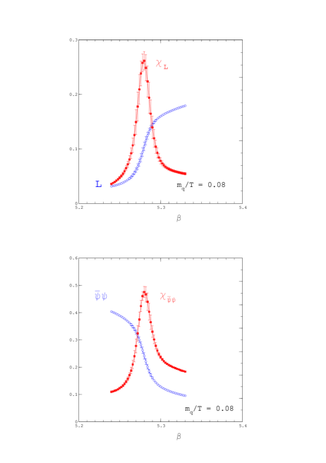
Figure 1: Order parameters for the chiral and deconfinement transitions (lower and upper figures, respectively) are plotted as a function of the inverse QCD coupling $\beta=6/g^{2}$. High (low) values of $\beta$ correspond to high (low) values of the temperature. The associated susceptibilities are also plotted in each case. Courtesy of [20].

2.3.2 Critical Exponents

An obvious question that one may pose, when faced with a phase transition, is what are the critical exponents that govern the transition? Pisarski and Wilczek suggested that the dynamics of QCD is controlled by an effective scalar Lagrangian, constructed along the lines of the linear $\sigma$ model [21], and, which for two flavors of quarks, has $SU(2)\otimes SU(2)=O(4)$ symmetry. Now, according to arguments of universality [22], only the symmetry structure and dimensionality determine the values of the critical exponents, i.e. one expects that one should obtain the critical exponents of a 3D $O(4)$ symmetric spin model. The task of studying the critical exponents has been undertaken by a lattice group [4]. Noting that the masses, which are responsible for explicit chiral symmetry breaking, play an analogous role to that of a magnetic field in the superconducting transition, these authors [3, 4] have adopted the convention of defining a scaled quark mass as $h=m_{q}/T$ and the reduced temperature $t=(T-T_{c})/T_{c}$. With this convention, the free energy density scales as

$$f(t,h)=-\frac{T}{V}\ln Z=b^{-1}f(b^{y_{t}}t,b^{y_{h}}h),$$ (27)

introducing the thermal $(y_{t})$ and magnetic $(y_{h})$ critical exponents. Here $b$ is an arbitrary scaling factor. There are various scaling relations that can be derived using Eq.(27). In particular, one can show that the chiral order parameter scales as

$$\langle\bar{\psi}\psi\rangle(t,h)=h^{1/\delta}F(z),$$ (28)

with $z=th^{1/\beta\delta}$, and the chiral susceptibility, defined as $\chi_{m}(t,h)=\partial\langle\bar{\psi}\psi\rangle/\partial m$, via

$$\chi_{m}(t,h)=\frac{1}{\delta}h^{\frac{1}{\delta}-1}[F(z)-\frac{z}{\beta}F^{\prime}(z)].$$ (29)

The more familiar critical exponents $\delta$ and $\beta$ are related to $y_{t}$ and $y_{h}$ via

$$\beta=\frac{(1-y_{h})}{y_{t}}\quad\quad{\rm and}\quad\quad\delta=\frac{y_{h}}{1-y_{h}}.$$ (30)

The heights of the peaks of the susceptibilities scale themselves with the behavior

$$\chi_{m}^{{\rm peak}}\sim m^{-z_{m}}\quad\quad{\rm and}\quad\quad\chi_{t}^{{\rm peak}}\sim m^{-z_{m}}$$ (31)

with $z_{m}=2-1/y_{h}$ and $z_{t}=(y_{t}-1)/y_{h}+1$.

	$y_{h}$	$y_{t}$	$z_{m}$	$z_{t}$
$O(4)$	0.83	0.45	0.79	0.34
$O(2)$	0.83	0.50	0.79	0.39
MF	$3/4$	$1/2$	$2/3$	$1/3$

Table 1: Critical exponents for $O(4)$, $O(2)$ and mean field theory (MF). Taken from [4].

The expected values for the critical exponents for the case of $O(4)$ symmetry, $O(2)$ symmetry, and mean field exponents (MF) are listed in Table I, in the form of $y_{h}$, $y_{t}$, and the corresponding values of $z_{m}$ and $z_{t}$. The $O(2)$ symmetry exponents are also listed, because at finite lattice spacing, the exact chiral symmetry of the staggered fermion action is $U(1)\simeq O(2)$. Only sufficiently close to the continuum limit does one expect to find $O(4)$ exponents.

The calculated results for the exponents themselves, evaluated on different spatially sized lattices, are summarized in Table 2. Comparing Tables 1 and 2, one sees that at this stage, no definitive statement about the symmetry of the underlying Lagrangian can be made from lattice gauge theory. This is an indicator that vital study in this field is still necessary to determine the underlying symmetry group conclusively. It is probably necessary to increase the lattice sizes and move to smaller masses.

	$8^{3}$	$12^{3}$	$16^{3}$
$z_{m}$	0.84(5)	1.06(7)	0.93(8)
$z_{t}$	0.63(7)	0.94(12)	0.85(12)

Table 2: Critical exponents, as a function of the lattice size. Taken from Ref.[4].

2.3.3 Meson screening masses and $U_{A}(1)$ restoration

One of the questions that has raised some theoretical interest in the last few years is whether the $U_{A}(1)$ symmetry, i.e. the symmetry $\psi\rightarrow e^{i\alpha\gamma_{5}}\psi$, which leads to the non-conserved current $A_{0}^{\mu}$ that is given in Eq.(20) is also restored at finite temperature, at some point. For three flavors, this occurs trivially. A demonstration of this, following Ref.[23] is given.

In SU(3), the statement that $U_{A}(1)$ is restored, implies that $m_{\pi}=m_{\eta^{\prime}}$. Since the masses of the particles are determined from the vacuum expectation values of the appropriate meson-meson correlators, we need to show only that

$$\langle\phi_{3}(x)\phi_{3}(0)\rangle=\langle\phi_{0}(x)\phi_{0}(0)\rangle,$$ (32)

where $\phi_{3}(x)=\bar{\psi}(x)i\gamma_{5}\lambda_{3}\psi(x)$ is the correlator for the $\pi_{0}$ and $\phi_{0}(x)=\bar{\psi}i\gamma_{5}\lambda_{0}\psi(x)$ is that for the $\eta^{\prime}$. If one considers the specific axial transformation

$$\psi(x)\rightarrow\psi^{\prime}(x)=e^{i\gamma_{5}(\sqrt{3}\lambda_{8}-\lambda_{3})\frac{\pi}{4}}\psi(x),$$ (33)

then, after a little algebra, one finds that the composite fields transform as

$$\phi_{3}(x)\rightarrow\phi^{\prime}{}_{3}(x)=\sqrt{\frac{2}{3}}\phi_{0}(x)+\sqrt{\frac{1}{3}}\phi_{8}.$$ (34)

The correlator composed of these composite fields itself then transforms as

$$\langle\phi_{3}(x)\phi_{3}(0)\rangle \rightarrow \langle\phi^{\prime}{}_{3}(x)\phi^{\prime}{}_{3}(0)\rangle$$

$$= \frac{2}{3}\langle\phi_{0}(x)\phi_{0}(0)\rangle+\frac{1}{3}\langle\phi_{8}(x)\phi_{8}(0)\rangle$$

$$+ \frac{\sqrt{2}}{3}\langle\phi_{0}(x)\phi_{8}(0)\rangle+\frac{\sqrt{2}}{3}\langle\phi_{8}(x)\phi_{0}(0)\rangle$$

The last two terms of this expression vanish, since the system is assumed to be $SU_{V}(3)$ symmetric. In addition, this implies that $\langle\phi_{3}(x)\phi_{3}(0)\rangle=\langle\phi_{8}(x)\phi_{8}(0)\rangle$, so that Eq.(LABEL:e:mult) implies that

$$\langle\phi_{0}(x)\phi_{0}(0)\rangle=\langle\phi_{3}(x)\phi_{3}(0)\rangle,$$ (36)

or that $m_{\eta^{\prime}}=m_{\pi}$.

In retrospect, it is simple to understand why the symmetry must be restored. Noting that mathematical constructions containing traces of fields preserve the symmetry, while determinants or antisymmetric functions violate it, one sees that the lowest order combination of fields that would violate $U_{A}(1)$ would involve the completely antisymmetric tensor, and consequently contain three field combinations. Since one requires here only two field operator combinations in order to construct a meson-meson correlator, this must be $U_{A}(1)$ invariant in the chirally restored phase. This leads to the definitive statement: for $n<N_{f}$, all $n$-point functions in the chirally restored phase are $U_{A}(1)$ invariant.

From the previous argument, it is evident that in SU(2) the situation is more complicated. There are two independent chiral multiplets in this case: $(\sigma,\vec{\pi})$ and $(\eta^{\prime},\vec{a}_{0})$. In lattice studies, the behavior of the masses of the $\pi$ and the $a_{0}$ have been calculated. Here the integral over the correlators has been studied,

$$\chi_{M_{i}}=\int d^{4}x\langle\phi_{i}(x)\phi_{i}(0)\rangle$$ (37)

for $M_{i}=\pi$ or $a_{0}$, and the leading behavior of these correlators is assumed to be $\chi_{M_{i}}\sim m_{M_{i}}^{-2}$. A plot of the “screening masses” obtained in this fashion is shown in Fig. 2 as a function of $6/g^{2}$, with $g$ the coupling in the QCD Lagrangian, which again represents increasing temperature over the region of the phase transition. It is interesting to note that the $\pi$ and $\sigma$ have become degenerate: in this picture, this occurs at some temperature slightly larger than $T_{c}$, with the $\sigma$ undershooting the $\pi$ curve and approaching it from below. That the $\sigma$ meson undershoots the $\pi$ curve is not expected from model calculations and may be a lattice artifact. This will be discussed in the following sections. One sees in Fig. 2 that the mass of the other scalar, the $a_{0}$, drops with temperature, but not as drastically as does the $\sigma$. One observes that it does not become degenerate with the $\pi$ and $\sigma$ over the temperature range indicated. Thus it does not appear from this particular calculation that $U_{A}(1)$ symmetry is restored in SU(2). An alternate approach, however, using the scaling arguments of Brown and Rho [24], does  however indicate a degeneracy at the transition temperature [4]. Thus, in this section once again, the question of the restoration of $U_{A}(1)$ symmetry is not resolved.

Figure 2: Meson screening masses plotted as a function of $\beta=6/g^{2}$. The critical value $\beta=\beta_{c}$ is indicated by the vertical line.

2.3.4 Bulk thermodynamic quantities.

One of the most important contributions that lattice physics is able to provide are calculations of bulk thermodynamic quantities. In particular, the energy density and pressure densities are given by

$$e=\frac{T^{2}}{V}\frac{\partial}{\partial T}\ln Z$$ (38)

and

$$p=T\frac{\partial}{\partial V}\ln Z$$ (39)

in terms of the partition function $Z$. In practice [25], the pressure density is obtained from integration of the difference of the action densities at zero and finite temperature,

$$\frac{p}{T^{4}}|_{\beta_{0}}^{\beta}=N_{\tau}^{4}\int_{\beta_{0}}^{\beta}d\beta(S_{0}-S_{T}).$$ (40)

Note that this quantity is defined in such a way that $p/T^{4}_{T=0}=0$, in contrast to setting the usual thermodynamic limit of Nernst, i.e. the entropy ${\cal S}(T=0)=0$ [26]. While this does not affect anything that follows, one should bear this in mind when making model comparisons, as will be done in Section 3.

In the following figures, we have chosen to illustrate the pressure and energy densities for lattice simulations that include quark degrees of freedom, rather than simply quenched QCD. In Fig. 3, we show the pressure density, plotted as a function of the scaled temperature, for four flavor QCD on a $16^{3}\times 4$ lattice. A comparison is made on varying the quark masses, and using quenched QCD, in the latter case with appropriate scaling of the number of degrees of freedom. One sees that there is a sharp rise in the pressure density at $T=T_{c}$, and the curve tends to the Stefan-Boltzmann limit, but does not reach it over the temperature range $(3.5T_{c})$ shown. The deviation from the ideal gas limit appears to be too large to be described by perturbation theory, suggesting here that the perturbative regime occurs for temperatures $T>>T_{c}$.

Figure 3: Pressure density, plotted as a function of the scaled temperature $T/T_{c}$. (Taken from [3].)

The energy density of four flavor QCD on a $16^{3}\times 4$ lattice is shown in Fig. 4. In this case, the energy density remains close to the ideal gas limit at temperatures of the order of $3T_{c}$, but overshoots it and approaches it from above for finite values of the quark mass. Whether this is a lattice artifact or not is presently unclear.

Figure 4: Energy density plotted as a function of the scaled temperature, $T/T_{c}$. (Taken from [3].)

In concluding this section, we see that lattice gauge simulations are reaching a point where one may obtain “exact” results that stem directly from the discretized QCD Lagrangian. These can be used as a guide for constructing simple models, and conversely, simple models and simple predictions based solely on symmetry considerations such as discussed here may be used as a guide for the interpretation of the numerical results. As has emerged here, there are still many questions that are open for study.

With this, we turn to a different approach which is regarded by its protagonists as being an exact low energy representation of QCD, viz. chiral perturbation theory and investige what is known at finite temperature.

2.4 Chiral perturbation theory

2.4.1 A brief introduction

Chiral perturbation theory starts with the premise that an effective Lagrangian for QCD at low temperatures can be written solely in terms of the observed baryonic (here mesonic) degrees of freedom, in such a way that global chiral symmetry is enforced. This is done in its most general form by collecting the mesonic degrees of freedom into the field

$$U(x)=\exp(i\pi^{a}\tau_{a}/F),$$ (41)

where $\pi^{a}$ are the $SU(2)$ pion fields, $\tau_{a}$ the Pauli matrices, and $F$ the pion decay constant, and contructing a Lagrangian density that is ordered in momenta. Such an expansion for the Lagrangian only starts at $O(p^{2})$, and must contain an even number of derivatives in order to be Lorentz invariant. Writing

$${\cal L}_{QCD}\rightarrow{\cal L}_{eff}={\cal L}_{eff}^{(2)}+{\cal L}_{eff}^{(4)}+{\cal L}_{eff}^{(6)}+\dots,$$ (42)

the lowest leading order term is

$${\cal L}_{eff}^{(2)}=\frac{1}{4}F^{2}{\rm tr}(\partial_{\mu}U\partial^{\mu}U^{\dagger}),$$ (43)

which, taken on its own, is the (non-renormalizable) sigma model. QCD, as we have already discussed, is however not completely invariant under chiral symmetry. There is an explicit breaking of the symmetry due to the presence of the current quark mass matrix. The symmetry breaking term is in general given as

$${\cal L}_{sb}=f(U,\partial U,\dots)\times m^{0},$$ (44)

where $m^{0}$ is the (real and diagonal) current quark mass matrix. One incorporates this into the effective Lagrangian by making not only an expansion in powers of the derivatives, but also in powers of $m^{0}$, i.e. ${\cal L}_{sb}\sim f(U)\times m^{0}$ to leading order. More precisely, this term takes the form (that is Lorentz and parity invariant)

$${\cal L}_{sb}=\frac{1}{2}F^{2}B{\rm tr}(m^{0}(U+U^{\dagger})),$$ (45)

introducing the new constant $B$. This is generally included in the definition of ${\cal L}_{eff}^{(2)}$, i.e.

$${\cal L}_{eff}^{(2)}=\frac{1}{4}F^{2}{\rm tr}(\partial_{\mu}U\partial^{\mu}U^{\dagger})+\frac{1}{2}F^{2}B{\rm tr}(m^{0}(U+U^{\dagger})).$$ (46)

In this reckoning, one can thus regard $m^{0}$ as being of $O(p^{2})$.

To make physical sense of the constant $B$, one may expand the field $U=\exp(i\pi\cdot\tau/F)$ in powers of the pion field $\pi$. The symmetry breaking part of the Lagrangian then becomes

$${\cal L}_{sb}=(m_{u}^{0}+m_{d}^{0})B[F^{2}-\frac{1}{2}\pi^{2}+\frac{1}{24}\pi^{4}F^{-2}+\dots]$$ (47)

The first term in this expansion gives the vacuum energy generated by the symmetry breaking. The second term generates the pion mass, while the higher order terms describe further interactions of the $\pi$ fields. By direct analogy with the QCD Hamiltonian, we know that the derivative of $H_{QCD}$ with respect to $m_{u}^{0}$ generates the operator $\bar{u}u$. Thus the derivative of the vacuum energy with respect to the current quark mass gives the vacuum expectation value of this operator. Applying this to ${\cal L}_{eff}$, one has

$$\langle 0|\bar{u}u|0\rangle=\langle 0|\bar{d}d|0\rangle=-F^{2}B\{1+O(m)\},$$ (48)

indicating that $B$ is related to the condensate. Since the pion mass is given as

$$m_{\pi}^{2}=(m_{u}^{0}+m_{u}^{0})B\{1+O(m)\},$$ (49)

one obtains the Gell-Mann-Oakes-Renner (GOR) relation [28],

$$F_{\pi}^{2}M_{\pi}^{2}=(m_{u}^{0}+m_{d}^{0})|\langle 0|\bar{u}u|0\rangle|$$ (50)

from Eqs.(48) and (49), on eliminating $B$.

To order $p^{4}$, the effective Lagrangian would contain two additional independent terms in the event that no current quark mass were present, i.e. one would include two new terms

$${\cal L}_{eff}^{(4)}=\frac{1}{4}l_{1}({\rm tr}\{\partial_{\mu}U^{\dagger}\partial^{\mu}U\})^{2}+\frac{1}{4}l_{2}{\rm tr}(\partial_{\mu}U^{\dagger}\partial_{\nu}U){\rm tr}(\partial^{\mu}U^{\dagger}\partial^{\nu}U).$$ (51)

with new low energy constants $l_{1}$ and $l_{2}$. Including the current quark mass matrix again to construct an explicit symmetry breaking terms requires the inclusion of further additional terms, as was the case for ${\cal L}^{(2)}_{eff}$. For most purposes, this is sufficient. However, to obtain the most general form from which all propagators can be derived, it is useful to introduce external fields into the Lagrange density. Here the essential additions are $v_{\mu}(x)$ and $a_{\mu}(x)$ that are vector and axial vector in nature and which can be regarded as being of order $p$. Then, using the original notation of Ref.[1], the complete set of terms that contribute to ${\cal L}_{eff}^{(4)}$ were worked out by these authors and found to be, for SU(3)

$${\cal L}_{eff}^{(4)} = L_{1}\langle\nabla_{\mu}U^{\dagger}\nabla^{\mu}U\rangle^{2}+L_{2}\langle\nabla_{\mu}U^{\dagger}\nabla_{\mu}U\rangle\langle\nabla^{\mu}U^{\dagger}\nabla^{\nu}U\rangle$$ (52)

$$+ L_{4}\langle\chi U^{\dagger}+\chi^{\dagger}U\rangle\langle\nabla U^{\dagger}\nabla^{\mu}U\rangle+L_{6}\langle\chi U^{\dagger}+\chi^{\dagger}U\rangle^{2}$$

$$+ L_{8}\langle\chi U^{\dagger}\chi U^{\dagger}+U\chi^{\dagger}U\chi^{+}\rangle+L_{10}\langle U^{\dagger}F^{\mu\nu}_{R}UF_{L\mu\nu}\rangle$$

$$+ H_{1}\langle F^{\mu\nu}_{R}F_{R\mu\nu}+F^{\mu\nu}_{L}F_{L\mu\nu}+H_{2}\langle\chi^{\dagger}\chi\rangle+L_{7}\langle\chi U^{\dagger}-U\chi^{\dagger}\rangle^{2}$$

$$+ L_{5}\langle\nabla_{\mu}U\nabla^{\mu}U^{\dagger}(\chi U^{\dagger}+U\chi^{\dagger})\rangle+iL_{9}\langle F^{L}_{\mu\nu}\nabla^{\mu}\nabla^{\nu}U^{\dagger}+F^{R}_{\mu\nu}\nabla^{\mu}\nabla^{\nu}U\rangle$$

$$+ L_{3}\langle\nabla_{\mu}U\nabla^{\mu}U^{\dagger}\nabla_{\nu}U\nabla^{\nu}.U^{\dagger}\rangle$$

where using a different notation to Eq. (51) now, the low energy constants $L_{1}$ to $L_{10}$, and $H_{1}$ and $H_{2}$ have been introduced. The angular brackets are a shorthand notation for the trace. In this expression, one notes that the covariant derivative that is constructed using the external field must now appear,

$$\nabla_{\mu}=\partial_{\mu}-i\{a_{\mu},U\},$$ (53)

and $F^{\mu\nu}$ is the field strength tensor constructed from the external field, i.e.

$$F^{\mu\nu}_{R,L}=\pm\partial^{\mu}a^{\nu}\mp\partial^{\nu}a^{\mu}-i[a^{\mu},a^{\nu}].$$ (54)

Terms involving the current quark mass have been summarized into the field $\chi=2B\hat{m}$, with $\hat{m}=(m^{u}_{0}+m^{d}_{0})/2$. Note that the low energy constants $L_{i}$ become renormalized when physical quantities are calculated, as this theory is perturbatively renormalizable order by order. A certain number of such physical quantities that are measured in experiment must then be used to fit the renormalized parameters at a given mass scale. Given definite values for these constants, predictions of other quantities can then be made.

Three ingredients are essential to any application that attempts to calculate quantities for chiral perturbation theory to a specific order. For example, should one wish to calculate to $O(p^{4})$, the following steps must be taken: (1) The general ${\cal L}^{(2)}_{eff}$ of order $p^{2}$ is to be used at both the tree and one loop level. (2) The general ${\cal L}^{(2)}_{eff}$ of order $p^{4}$ is to be used only at tree level. (3) A renormalization program must be implemented to make physical predictions. The extension of this procedure to higher powers in $p^{2}$ is obvious.

Let us look at a standard example for the derivation of the pion mass [29]. In what follows, we denote the low energy constants appropriate to SU(2) two flavors as being $L_{i}^{(2)}$. If one expands the Lagrangians ${\cal L}_{eff}^{(2)}$ and ${\cal L}_{eff}^{(4)}$ in terms of the pion fields, one finds

$${\cal L}^{(2)}_{eff}=\frac{2}{3}[\partial^{\mu}\pi\partial_{\mu}\pi-m^{2}\pi\cdot\pi]+\frac{m^{2}}{6F^{2}}[(\pi\cdot\partial^{\mu}\pi)(\pi\cdot\partial_{\mu}\pi)-(\pi\cdot\pi)(\partial^{\mu}\pi\cdot\partial_{\mu}\pi)]+O(\pi^{6}),$$ (55)

while

$${\cal L}^{(4)}_{eff} = \frac{m^{2}}{f^{2}}[16L_{4}^{(2)}+8L_{5}^{(2)}]\frac{1}{2}\partial_{\mu}\pi\cdot\partial^{\mu}\pi$$ (56)

$$- \frac{m^{2}}{F^{2}}[32L_{6}^{(2)}+16L_{8}^{(2)}]\frac{1}{2}\hat{m}^{2}\pi\cdot\pi+O(\phi^{4}).$$

The terms in ${\cal L}^{(4)}_{eff}$ that are of order $\pi^{4}$ contribute to physical quantities via one loop diagrams and one therefore does not need to consider these in a calculation to order $O(p^{4})$. What is required however, are the one loop diagrams that are generated by ${\cal L}_{eff}^{(2)}$. For a calculation of the the renormalized pion mass, however, one can avoid evaluating any diagrams at all by simply considering all possible contractions of two fields in these terms in ${\cal L}^{(4)}_{eff}$, to arrive at an “effective” effective Lagrangian, that takes the form

$${\cal L}^{(4)}_{eff} = \frac{1}{2}\partial^{\mu}\pi\cdot\partial_{\mu}\pi-\frac{1}{2}m^{2}\pi\cdot\pi+\frac{5m_{\pi}^{2}}{12m^{2}}I(m_{\pi}^{2})\pi\cdot\pi$$

$$+ \frac{1}{6F^{2}}(\delta_{ik}\delta_{jl}-\delta_{il}\delta_{kl})I(m^{2}_{\pi})(\delta_{ij}\partial^{\mu}\pi_{k}\partial_{\mu}\pi_{l}+\delta_{kl}m_{\pi}^{2}\pi_{i}\pi_{j})$$

$$+ \frac{1}{2}\partial_{\mu}\pi\partial^{\mu}\pi\frac{m_{\pi}^{2}}{F_{\pi}^{2}}[16L_{4}^{(2)}+8L_{5}^{(2)}]-\frac{1}{2}m_{\pi}^{2}\pi\cdot\pi\frac{m_{\pi}^{2}}{F_{\pi}^{2}}[32L_{6}^{(2)}+16L_{8}^{(2)}].$$

In obtaining this result, the Feynman propagator

$$i\Delta_{Fjk}(0)=\langle 0|\pi_{j}(x)\pi_{k}(x)|0\rangle=\delta_{jk}I(m_{\pi}^{2})$$ (58)

has been introduced and is written in terms of the integral

$$I(m_{\pi}^{2})=\mu^{4-d}\int\frac{d^{d}k}{(2\pi)^{d}}\frac{i}{k^{2}-m_{\pi}^{2}}=\mu^{4-d}(4\pi)^{d/2}\Gamma(1-\frac{d}{2})(m_{\pi}^{2})^{\frac{d}{2}-1}$$ (59)

that is treated with dimensional regularization, $d$ being an arbitrary dimension. In addition, use has been made of the fact that derivatives of the Feynman propagator, defined as

$$-\partial_{\mu}\partial_{\nu}i\Delta_{Fjk}(0)=\langle 0|\partial_{\mu}\pi_{j}(x)\partial_{\nu}\pi_{k}(x)|0\rangle=\delta_{ij}I_{\mu\nu}(m_{\pi}^{2})$$ (60)

can be expressed in terms of the integral $I(m_{\pi}^{2})$ via

$$I_{\mu\nu}(m_{\pi}^{2})=\mu^{4-d}\int\frac{d^{d}k}{(2\pi)^{d}}k_{\mu}k_{\nu}\frac{i}{k^{2}-m_{\pi}^{2}}=g_{\mu\nu}\frac{m_{\pi}^{2}}{d}I(m_{\pi}^{2}).$$ (61)

Regrouping the kinetic and mass terms, Eq.(LABEL:e:effeff) becomes

$${\cal L}_{eff} = \frac{1}{2}\partial^{\mu}\pi\cdot\partial_{\mu}\pi[1+(16L_{4}^{(2)}+8L_{5}^{(2)})\frac{m_{\pi}^{2}}{F_{\pi}^{2}}-\frac{2}{3F_{\pi}^{2}}I(m_{\pi}^{2})]$$ (62)

$$- \frac{1}{2}m^{2}\pi\cdot\pi[1+(32L_{6}^{(2)}+16L_{8}^{(2)})\frac{m_{\pi}^{2}}{F_{\pi}^{2}}-\frac{1}{6F_{\pi}^{2}}I(m_{\pi}^{2})].$$

By expanding this expression in powers of $d-4$ and renormalizing the pion field as $\pi_{r}=Z_{\pi}^{-1/2}\pi$, with

$$Z_{\pi}=1-\frac{8m_{\pi}^{2}}{F_{\pi}^{2}}(2L_{4}^{(2)}+L_{5}^{(2)})+\frac{m_{\pi}^{2}}{24\pi^{2}F_{\pi}^{2}}[\frac{2}{d-4}+\gamma-1-\ln 4\pi+\ln\frac{m_{\pi}^{2}}{\mu^{2}}],$$ (63)

one obtains the canonical form for the effective Lagrangian for pion fields,

$${\cal L}_{eff}=\frac{1}{2}\partial_{\mu}\pi_{r}\partial^{u}\pi_{r}-\frac{1}{2}M_{\pi}^{2}\pi_{r}\cdot\pi_{r},$$ (64)

with the identification of the physical pion mass as

$$M_{\pi}^{2}=m^{2}[1+\frac{m_{\pi}^{2}}{32\pi^{2}F_{\pi}^{2}}\ln\frac{m_{\pi}^{2}}{\mu^{2}}-\frac{8m_{\pi}^{2}}{F_{\pi}^{2}}L_{comb}].$$ (65)

Here $L_{comb}=2L_{4}^{(2)}{}^{r}+L_{5}^{(2)}{}^{r}-4L_{6}^{(2)}{}^{r}-2L_{8}^{(2)}{}^{r}$. In the original paper of Gasser and Leutwyler [1], $M_{\pi}^{2}$ was not obtained in this fashion, but rather from the expansion of the Fourier transform of the axial vector correlator, which has the form

$$J_{\mu\nu}^{ik}(p) = i\int d^{4}se^{ip(x-y)}\langle 0|TA_{\mu}^{i}(x)A_{\nu}^{k}(y)|0\rangle$$ (66)

$$= \delta^{ik}\{\frac{p_{\mu}p_{\nu}F_{\pi}^{2}}{M_{\pi}^{2}-p^{2}}+\dots\},$$

where $A_{\mu}^{i}(x)=\bar{\psi}(x)\gamma_{\mu}\gamma_{5}\frac{\tau^{i}}{2}\psi(x)$. From this expression, the corresponding expansion for $F_{\pi}$ has also been obtained.

2.4.2 Cool chiral perturbation theory

The evaluation of the condensate density at finite temperature was first carried out by Gerber and Leutwyler [5]. In their calculation, which involves ${\cal L}^{(2)}_{eff}$ and ${\cal L}^{(4)}_{eff}$, they find that the first term in the behavior of the condensate with temperature is quadratically decreasing, i.e.

$$\langle\bar{q}q\rangle=\langle 0|\bar{q}q|0\rangle_{T=0}[1-\frac{T^{2}}{8F^{2}}-\frac{T^{4}}{384F^{4}}-\frac{T^{6}}{288F^{6}}\ln\frac{\Lambda_{q}}{T}+O(T^{8})].$$ (67)

This is a result that has been obtained under the assumption that quarks are massless, i.e. in the chiral limit. $\Lambda_{q}$ is a scale factor constructed from the renomalized low energy constants, and is expected to be of the order of $\Lambda_{q}=360..580$ MeV.

In a recent publication, Toublan [6] has investigated pion static properties with the aim of obtaining $O(p^{6})$ accuracy in all quantities and to then verify the Gell-Mann–Oakes–Renner (GOR) [28] relation at finite temperature. To do so, the tree, one loop and two loop diagrams of ${\cal L}^{(2)}_{eff}$ are required, the tree and one loop graphs of ${\cal L}^{(4)}_{eff}$ are required plus the tree level graphs of ${\cal L}^{(6)}_{eff}$. In doing so, the result of Eq.(67) has been reconfirmed. In addition, the mass $M_{\pi}(T)$ and pion decay constant as a function of temperature are also evaluated, using the finite temperature axial vector correlator. In total, thirty-six Feynman graphs contribute to the correlator at this order! However, in the chiral limit, one is still lucky enough to have simple analytic forms for the temperature dependence. One finds

$$\frac{M_{\pi}^{2}(T)}{M_{\pi}}=1+\frac{T^{2}}{24F^{2}}-\frac{T^{4}}{36F^{4}}\ln\frac{\Lambda_{M}}{T}+O(T^{6}),$$ (68)

while

$$\frac{Re[F_{\pi}^{t}(T)]^{2}}{F_{\pi}^{2}}|_{\hat{m}=0}=1-\frac{T^{2}}{6F^{2}}+\frac{T^{4}}{36F^{4}}\ln\frac{\Lambda_{T}}{T}+O(T^{6}).$$ (69)

and

$$\frac{Re[F_{\pi}^{t}(T)-F_{\pi}^{s}(T)]}{F_{\pi}}|_{\hat{m}=0}=\frac{T^{4}}{27F^{4}}\ln{\Lambda_{\Delta}}T+O(T^{6}),$$ (70)

where $\Lambda_{M,T,\Delta}$ are various scales, whose sizes are determined by the renormalized couplings $L_{1}^{r}\dots L_{10}^{r}$ that are a function of scale. They are determined numerically to be $\Lambda_{M}\simeq 1.9$ GeV, $\Lambda_{T}\simeq 2.3$ GeV, and $\Lambda_{\Delta}=1.8$ GeV. Note that, at finite temperature, there is a separation of “temporal” and “spatial” pion decay constants. This comes about since Lorentz invariance is not maintained in a heat bath and the the singular part of the axial two point function takes the form

$$A_{\mu\nu}(q,T)=-\frac{f_{\mu}(q,T)f_{\nu}(q,T)}{q_{0}^{2}-\Omega^{2}(\vec{q},T)}$$ (71)

where

$$f_{0}(q,T)=q_{0}F_{t}(q,T)\quad\quad{\rm}\quad\quad f_{i}(q,T)=q_{i}F_{s}(q,T),$$ (72)

with $i=1..3$, and the decay constants $F_{\pi}^{s,t}$ are defined as

$$F_{\pi}^{s,t}(T)=F_{s,t}(\vec{q},T)|_{\vec{q}=0}.$$ (73)

The GOR relation is modified so as to read [6]

$$\lim_{\hat{m}\rightarrow 0}\frac{M_{\pi}^{2}(T){\rm Re}[F^{t}_{\pi}(T)]^{2}}{\hat{m}\langle\bar{q}q\rangle_{T}}=-1+O(T^{6}).$$ (74)

For this reason, we show graphs for $M_{\pi}^{2}(T)/M_{\pi}^{2}$ and ${\rm Re}[F_{\pi}^{t}(T)]^{2}/F_{\pi}^{2}$, as a function of temperature in Figs. 5 and 6. The tree level result is given (dotted curve), together with the one loop computation (upper dashed line in Fig. 5, lower dashed line in Fig. 6) and the two loop approximation (solid curve). In both of these figures, a non-zero value of the quark mass has been assumed for these curves. In the chiral limit, one finds the lower (upper) dashed curve in Fig. 5 (6). What is evident from these two figures, is that chiral perturbation theory is not converging and appears to provide an oscillating series for these quantities. Thus for larger values of the temperature, $T>100$ MeV say, one sees that the pion mass decreases with temperature in the two loop approximation, in contradistinction with the one loop result, the lattice results of the last section, and also in contradistinction with the model results obtained in the Nambu–Jona-Lasinio model, which will be presented later on in the following section. Convergence at temperatures in this range appears to be problematic, which is perhaps an indication that the series is at best asymptotic, or changes its nature due to the onset of the phase transition. In this range, one expects non-analytic behavior and it is unreasonable to expect a perturbation analysis to succeed. These curves clearly indicate that ChPT at finite temperature can at best be regarded as cool, so that the fundamental behavior at low temperatures sets a constraint on the finite temperature behavior of would-be effective models.

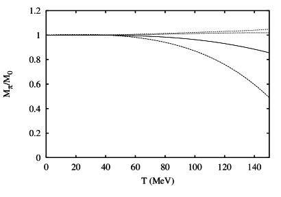
Figure 5: The pion mass, scaled by its value at $T=0$ is shown as a function of the temperature.

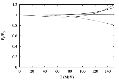
Figure 6: The pion decay constant, scaled by its value at $T=0$ is shown as a function of the temperature.

3 The Nambu–Jona-Lasinio model

The Nambu–Jona-Lasinio (NJL) model has been reviewed in detail by several authors from different viewpoints [8, 9, 10], and consequently I do not wish to present any detail of this model other that a basic introduction here. Rather the purpose of this chapter is to illustrate that with the simple equations requiring little computational time, one can reproduce all the main features of the static properties that have been so arduously extracted from years of labor on the lattice. It is extremely encouraging to have a simple model that can be handled semi-analytically – one gains a tremendous amount of insight into the actual functioning of the mechanism of dynamical symmetry breaking and the consequences thereof.

Nevertheless, the NJL model is simply a model – in contrast to the results of the previous section, which are regarded as “factual”, this section can only give model-dependent results. Accordingly it is only equitable to indicate, in addition to the successes provided by this approach, the failings also. These become obvious when examining bulk thermodynamic properties, such as pressure, energy and entropy densities, and will be discussed in what follows.

We shall then turn to dynamic properties, and examine the temperature dependence of scattering amplitudes in the quark-antiquark channel, which displays a divergence which we term critical scattering, in analogy to the phenomenon of critical opalescence that is observed in light scattering.

3.1 Order parameter

We first consider the order parameter for the chiral transition that is obtained from the NJL Lagrangian, which, for two flavors of quarks, is taken to be

$${\cal L}_{NJL}=\bar{\psi}(x)(i\not\!\partial-m_{0})\psi(x)+G[(\bar{\psi}\psi)^{2}+(\bar{\psi}i\gamma_{5}\tau\psi)^{2}],$$ (75)

where $G$ is a dimensionful coupling strength, and $m_{0}$ denotes the common current quark mass for $u$ and $d$ quarks. For three flavors of quarks, we use

$${\cal L}_{NJL} = \bar{\psi}(x)(i\not\!\partial-m_{f}^{0})\psi(x)+G\sum_{a=0}^{8}[(\bar{\psi}\lambda^{a}\psi)^{2}+(\bar{\psi}\lambda^{a}\gamma_{5}\psi)^{2}]$$ (76)

$$- K\{{\rm det}\bar{\psi}(1+\gamma_{5})\psi+{\rm det}\bar{\psi}(1-\gamma_{5})\psi\}.$$

Here $G$ and $K$ both are dimensionful coupling strengths and $m_{f}^{0}={\rm diag}(m_{0}^{u},m_{0}^{d},m_{0}^{s})$. The self-energy, in the mean field approximation, that corresponds to the lowest order term in an expansion in the inverse number of colors $N_{c}$ [12, 13], is given as

$$m=m_{0}-2G\langle\langle\bar{\psi}\psi\rangle\rangle,$$ (77)

and the condensate is given explicitly as

$$\langle\langle\bar{\psi}\psi\rangle\rangle=\frac{N_{c}N_{f}}{\pi^{2}}\int_{0}^{\Lambda}\frac{p^{2}}{E_{p}}[1-f^{-}(p,\mu)-f^{+}(p,\mu)],$$ (78)

with

$$f^{\pm}(p,\mu)=\frac{1}{[1+\exp\ \beta(E_{p}\pm\mu)]}.$$ (79)

One sees that the condensate is directly proportional to the value of the dynamically generated mass, in the event that the current quark mass is zero. Although the situation is more complicated in SU(3), where the dynamically generated quark masses satisfy coupled equations,

$$m_{i} = m_{i}^{0}-\frac{GN_{c}}{\pi^{2}}m_{i}A(m_{i},\mu_{i})+\frac{KN_{c}^{2}}{\pi^{2}}m_{j}m_{k}A(m_{j},\mu_{j})A(m_{k},\mu_{k}),$$ (80)

$$i\neq j\neq k$$

and the function

$$A(m_{f},\mu_{f})=\frac{16\pi^{2}}{\beta}\sum_{n}e^{i\omega_{n}\eta}\int_{|\vec{p}|<\Lambda}\frac{d^{3}p}{(2\pi)^{3}}\frac{1}{(i\omega_{n}+\mu_{f})^{2}-E_{f}^{2}}$$ (81)

is proportional to the condensate density for a specific flavor,

$$A(m_{f},\mu_{f})\sim\langle\langle\bar{\psi}\psi\rangle\rangle_{f},$$ (82)

the dynamically generated quark masses are equivalently order parameters of the phase transition, and we therefore plot these. They are shown here only for the SU(3) case, in Fig. 7, for a finite value of the current quark mass [30]. As expected, the phase transition that occurs in the chiral limit is washed out and becomes a cross over. Another feature that emerges in this model is that the strange quark mass remains large, even at temperatures $T\sim 300$ MeV, and does not reach its current mass value of 150 MeV until $T>>T_{c}$.

Figure 7: Temperature dependence of the constituent quark masses. The solid line refers to the light quarks, the dashed to the strange quark [30].

3.2 Meson masses

The meson masses for the scalar and pseudosalar sectors are determined via the well-known method of evaluating the quark-antiquark scattering amplitude in the random phase approximation, and searching for poles of this function. This involves knowing only the irreducible polarization function that one can construct from a single quark loop, the details of which can be found, for example, in [9, 10, 30]. One finds the masses that are shown in Figs. 8 and 9 for the pseudoscalar and scalar sectors, respectively. In Fig. 8, $2m_{q}$ is plotted in addition to $m_{\pi}$. The point at which these two curves cross is called the Mott temperature, $T_{M_{\pi}}$. For $T>T_{M_{\pi}}$, the pion is no longer a bound state, but is a resonance, with a finite width that is not shown here. Similarly we have plotted $m_{q}+m_{s}$, from which the kaonic Mott temperature $T_{M_{K}}$ is defined. For $T>>T_{M_{K}}$, the kaon is also a resonance with a finite width

Figure 8: Temperature dependence of the pseudoscalar meson masses, as well as that of $2m_{q}$ and $m_{q}+m_{s}$. [30].

Figure 9: Temperature dependence of the scalar meson masses and $2m_{q}$ [30].

These graphs deserve some comment. Firstly let us compare them with the figure showing the meson masses obtained via lattice gauge theory, Fig. 2. We note first that there are some fundamental differences in obtaining these graphs: (a) Figs. 8 and 9 show so-called pole masses, while Fig. 2 gives screening  masses. Nevertheless, it has been shown that, in the NJL model, the temperature behavior of screening masses and pole masses is qualitatively similar [31], although quantitatively somewhat different. Since we cannot hope for any quantitative agreement at this stage, it is justifiable to make a comparison. (b) The NJL model calculation shown is for SU(3), while the lattice calculation is SU(2). With these points in mind, note that the $\sigma$ and $\pi$ mesons from figures 8 and 9 become degenerate at high temperatures, as observed also in Fig. 2. However, there is no undershooting of the $\sigma$ meson. The meson labelled $m_{\sigma_{\pi}}$ of Fig. 8 corresponds to the $a_{0}$ of Fig. 2. Here one observes qualitatively the same behavior, i.e. that this scalar meson also decreases strongly in the phase transition region. Thus one has an aesthetically pleasing agreement between the NJL model and the results obtained by lattice gauge theory for meson masses at this level.

A direct comparison of Fig. 7 with the results of chiral perturbation theory, i.e. with Fig. 5 is problematic. We simply make some comments: (a) the physics underlying Figs. 5 and 7 is completely different. Fig. 5 is obtained by constructing meson loops (the mesons are regarded as structureless point-like objects), while in Fig. 7, the pion is constructed from a quark-antiquark loop. Meson loops form corrections to this calculation and would be of the next order in $1/N_{c}$. Such corrections have in fact been evaluated, and it has been found that the leading order $T^{2}$ dependence of Eq.(68) is recovered [32]. The fact that in the final analysis the curve of $M_{\pi}$ as a function of temperature is finally decreasing for chiral perturbation theory in Fig. 5, is in strong contradiction to both Figs. 2 and 8.

3.3 Bulk thermodynamic quantities

In the last subsection, we have indicated the successes of the NJL model in calculating the order parameter and masses as a function of temperature. In this subsection, we turn to bulk thermodynamic quantities. Here we will see that the model does not do as well, and that the lack of confinement makes itself strongly evident at low temperatures, while the cutoff of the model is a hindrance at high temperatures. We start with the thermodynamical potential $\Omega$, calculated in the grand canonical ensemble. Given an interaction between fermions that is 4-point in nature such as in Eq.(75), $\Omega$ can be calculated quite generally as [10, 33]

$$\Omega=\Omega_{0}+\int_{0}^{1}\frac{d\lambda}{\lambda}\frac{1}{2}\int\frac{d^{3}p}{(2\pi)^{3}}\frac{1}{\beta}\sum_{n}\exp(i\nu_{n}\eta){\rm Tr}[\Sigma^{\lambda}(\nu_{n},\vec{p})S^{\lambda}(\nu_{n},\vec{p})],$$ (83)

where $\Omega_{0}$ is the thermodynamic potential in the absence of interactions, and $\sum^{\lambda}$ and $S^{\lambda}$ designate the Matsubara self-energy and Green function associated with the system. The superscript $\lambda$ refers to the fact that both $S$ and $\Sigma$ are to be evaluated with the introduction of an artifical coupling that multiplies the interaction Lagrangian ${\cal L}_{int}$. The Matsubara frequencies for fermions are, as required, odd, i.e. $\nu_{n}=(2n+1)\pi/\beta$, with $n=0,\pm 1,\pm 2\pm 3\dots$.

For the NJL Lagrangian of Eq.(75), in the mean field approximation, it is not necessary to apply Eq.(83). A straightforward calculation gives

$$\Omega=\Omega_{q}=-2N_{c}N_{f}\int\frac{d^{3}p}{(2\pi)^{3}}E_{p}-\frac{2N_{c}N_{f}}{\beta}\int\frac{d^{3}p}{(2\pi)^{3}}\ln[1+e^{-\beta(E_{p}+\mu)}][1+e^{-\beta(E_{p}-\mu)}],$$ (84)

with $E^{2}_{p}=\vec{p}^{2}+m^{2}$. As is evident from the label $q$, this appears to be a thermodynamic potential generated solely by the quark degrees of freedom.

We note also that the thermodyamical properties can only be measured relative to the physical vacuum,

$$\Omega^{phys}_{vac}=\Omega(T=0,\mu=0,m(0,0)),$$ (85)

which, for the mean field approximation, corresponds to

$$(\Omega^{phys}_{vac})_{mf}=\frac{(m-m_{0})}{4G}-2N_{c}N_{f}\int\frac{d^{3}p}{(2\pi)^{3}}E_{p}.$$ (86)

To introduce mesonic  degrees of freedom, it is necessary to go beyond the mean field approximation to include the next set of terms in the $1/N_{c}$ expansion. The self-energy in this case includes effective interactions in both the scalar and pseudoscalar channels [34],

$$\Sigma_{fl}^{\lambda}(\nu_{n},\vec{p})= - \frac{1}{\beta}\sum_{n^{\prime}}\int\frac{d^{3}q}{(2\pi)^{3}}[S(\nu_{n^{\prime}},\vec{q})V_{\sigma}^{\lambda}(\nu_{n}-\nu_{n^{\prime}},\vec{p}-\vec{q})$$ (87)

$$+ i\gamma_{5}\vec{\tau}S(\nu_{n^{\prime}},\vec{q})i\gamma_{5}\vec{\tau}V_{\pi}^{\lambda}(\nu_{n}-\nu_{n^{\prime}},\vec{p}-\vec{q})],$$

and is constructed on summing the Fock and infinite RPA series that contribute to the self-energy in this order. Here

$$V_{M}^{\lambda}(\omega,\vec{q})=-2G\lambda[1-2G\lambda\Pi_{M}(\omega,\vec{q})]^{-1},$$ (88)

and the irreducible polarization in the mesonic channel

$$\Pi_{M}(\omega_{m},\vec{p})=\int\frac{d^{3}q}{(2\pi)^{3}}\frac{1}{\beta}\sum_{n}{\rm Tr}\Gamma_{M}S(\nu_{n}+\omega_{m},\vec{q}+\vec{p})\Gamma_{M}S(\nu_{n},\vec{q}),$$ (89)

is determined by the vertex $\Gamma_{M}$ for that channel. Inserting Eq.(87) into Eq.(83) yields the fluctuating part of the thermodynamic potential,

$$\Omega_{fl}=\sum_{m}\frac{N_{M}}{2}\int\frac{d^{3}p}{(2\pi)^{3}}\frac{1}{\beta}\sum_{n}e^{i\omega_{n}\eta}\ln[1-2G\Pi_{M}(\omega_{n},\vec{p})].$$ (90)

The nature of this term is revealed on performing the frequency sum. One has

$$\Omega_{fl}=\Omega_{\pi}+\Omega_{\sigma},$$ (91)

where, for each species $M=\pi$ or $\sigma$,

$$\Omega_{M}= - N_{M}\int\frac{d^{3}p}{(2\pi)^{3}}\int_{0}^{\infty}d\omega[\frac{1}{2}\omega+\frac{1}{\beta}\ln(1-e^{-\beta\omega})]\frac{1}{2\pi i}$$ (92)

$$\times\frac{d}{d\omega}\ln\frac{1-2G\Pi_{M}(\omega+i\epsilon,\vec{p})}{1-2G\Pi_{M}(\omega-i\epsilon,\vec{p})}.$$

Some analysis shows that a simple approximation for the polarization near the pole, i.e.

$$1-2G\Pi_{M}(\omega,\vec{p})=(\omega^{2}-E_{M}^{2})\times{\rm const}$$ (93)

leads to

$$\Omega_{M}=N_{M}\int\frac{d^{3}p}{(2\pi)^{3}}[\frac{1}{2}E_{M}+\frac{1}{\beta}\ln(1-e^{-\beta E_{M}})],$$ (94)

exactly as one would expect for the thermodynamic potential given bosonic degrees of freedom. The pole approximation is however insufficient, as one integrates over all energies, and in practice, the fact that the bound states also become delocalized resonances at the Mott point must also be accounted for. This has been done in introducing phase shifts in each channel [34].

In order to calculate the pressure, the physical vacuum given by Eq.(85) must be reevaluated to include a term from $\Omega_{fl}$. One now has

$$\Omega^{phys}_{vac}=(\Omega^{phys}_{vac})_{mf}+(\Omega^{phys}_{vac})_{fl}.$$ (95)

and the pressure density is now

$$p=-\Omega_{q}-\Omega_{fl}+\Omega^{phys}_{vac}.$$ (96)

In Figs. 10 and 11, the pressure and associated energy densities evaluated from this thermodynamic potential are shown.

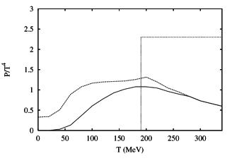
Figure 10: The pressure density, scaled by $T^{4}$, is shown as a function of temperature. The lower curve is for the mean field case only, the upper includes fluctuations (mesons). The vertical line indicates the critical temperature and the horizontal one the Stefan-Boltzmann limit for an ideal quark gas [34].

In Fig. 10, one sees that the lower curve, corresponding to the mean field approximation calculation represents the quark degrees of freedom. There is an appreciable pressure that arises from this term, i.e. from the quark degrees of freedom, for temperatures $T<T_{c}$, which is indicated by the vertical line. Including mesonic degrees of freedom rectifies the behavior at small temperatures, but still leaves a large intermediate range of temperatures $T<T_{c}$ that is dominated by these unphysical quark degrees of freedom. This is thus a direct consequence of the missing feature of confinement. The sharp rise in the pressure density shown in Fig. 3 cannot be modelled by a non-confining theory. At high temperatures, $T>T_{c}$, there is a small contribution from the mesonic degrees of freedom, that exist as correlated states with a finite width in the plasma. The main contribution arises however here from the quark degrees of freedom. The actual value obtained for the pressure density underestimates the Stefan-Boltzmann limit (shown as a horizontal line), since there is a finite cutoff on the quark momenta. Relaxing this constraint would lead to the pressure density approaching a constant.

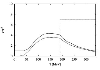
Figure 11: The energy density, scaled by $T^{4}$, is shown as a function of temperature. The lower curve is for the mean field case only, the upper includes fluctuations (mesons). The vertical line indicates the critical temperature and the horizontal one the Stefan-Boltzmann limit for an ideal quark gas [34].

Similar comments can be made for the energy density: the intermediate temperature range $50$MeV$<T<T_{c}$ is dominated by quark degrees of freedom, indicating the lack of confinement. The high temperature values $T>T_{c}$ do not approach the Stefan-Boltzmann limit, due to the cutoff.

In concluding this subsection, one sees that one needs to include confinement in some fashion in order to be able to regain the lattice picture. From a thermodynamic point of view, the high temperature regime about $T\simeq T_{c}$ is probably best described by the model, in the sense that only quark degrees of freedom plus correlated mesonic states are present. In the next subsection, we thus study elastic quark-antiquark scattering about this point and indicate that a divergence occurs in the cross-section at $T=T_{M}$ and that the phenomenon of critical scattering as a consequence of the chiral phase transition is observed.

3.4 Critical opalescence in the quark-antiquark channel

In this section, we examine the behavior of the quark-antiquark scattering amplitude in the NJL model in the vicinity of the Mott temperature, which replaces the critical temperature when finite current quark masses are used. In SU(3), there are seven independent processes out of a total of fifteen for quark-antiquark scattering, taking isospin and charge conjugation symmetry into account. These are listed in Table 3. Mesons that can be exchanged in the $s$ and $t$ channels, as are given by the Feynman diagrams of Fig. 12 are also listed.

Process	Exchanged mesons ($s$ channel)	Exchanged mesons ($t$ channel)
$u\bar{d}\rightarrow u\bar{d}$	$\pi$, $\sigma_{\pi}$	$\pi$, $\eta$, $\eta^{\prime}$, $\sigma_{\pi}$, $\sigma$, $\sigma^{\prime}$
$u\bar{s}\rightarrow u\bar{s}$	$K$, $\sigma_{K}$	$\eta$, $\eta^{\prime}$, $\sigma$, $\sigma^{\prime}$
$u\bar{u}\rightarrow u\bar{u}$	$\pi$, $\eta$, $\eta^{\prime}$, $\sigma_{\pi}$, $\sigma$, $\sigma^{\prime}$	$\pi$, $\eta$, $\eta^{\prime}$, $\sigma_{\pi}$, $\sigma$, $\sigma^{\prime}$
$u\bar{u}\rightarrow d\bar{d}$	$\pi$, $\eta$, $\eta^{\prime}$, $\sigma_{\pi}$, $\sigma$, $\sigma^{\prime}$	$\pi$, $\sigma_{\pi}$
$u\bar{u}\rightarrow s\bar{s}$	$\eta$, $\eta^{\prime}$, $\sigma$, $\sigma^{\prime}$	$K$, $\sigma_{K}$
$s\bar{s}\rightarrow u\bar{u}$	$\eta$, $\eta^{\prime}$, $\sigma$, $\sigma^{\prime}$	$K$, $\sigma_{K}$
$s\bar{s}\rightarrow s\bar{s}$	$\eta$, $\eta^{\prime}$, $\sigma$, $\sigma^{\prime}$	$K$, $\sigma_{K}$

Table 3: Independent processes for $q\bar{q}$ scattering.

Figure 12: Feynman diagrams for elastic $q\bar{q}$ scattering within the NJl model in an expansion to lowest order in $1/N_{c}$.

The transition amplitudes can be written as

$$-i{\cal M}_{s} = \delta_{c_{1},c_{2}}\delta_{c_{3},c_{4}}\bar{v}(p_{2})Tu(p_{1})[i{\cal D}_{s}^{S}(p_{1}+p_{2})]\bar{u}(p_{3})Tv(p_{4})$$

$$+\delta_{c_{1},c_{2}}\delta_{c_{3},c_{4}}\bar{v}(p_{2})(i\gamma_{5}T)u(p_{1})[i{\cal D}_{s}^{P}(p_{1}+p_{2})]\bar{u}(p_{3})(i\gamma_{5}T)v(p_{4}),$$

(97)

and

$$-iM_{t} = \delta_{c_{1},c_{3}}\delta_{c_{2},c_{4}}\bar{u}(p_{3})Tu(p_{1})[i{\cal D}_{t}^{S}(p_{1}-p_{3})]\bar{v}(p_{2})Tv(p_{4})$$

$$\delta_{c_{1},c_{3}}\delta_{c_{2},c_{4}}\bar{u}(p_{3})(i\gamma_{5}T)u(p_{1})[i{\cal D}_{t}^{P}(p_{1}-p_{3})]\bar{v}(p_{2})(i\gamma_{5}T)v(p_{4}),$$

where $T$ selects the isospin eigenvalue for a particular channel, and $D_{s,t}^{S,P}$ is the $s$ or $t$ channel, scalar or pseudoscalar quark-antiquark scattering amplitude, and which can be constructed from the corresponding polarization function. It has a simple form, for example [9]

$${\cal D}_{\pi}(p_{0},\vec{p})=\frac{2G^{eff}}{1-2G^{eff}\Pi^{P}_{u\bar{u}}(p_{0},\vec{p})},$$ (99)

where $G^{eff}$ is an effective SU(3) coupling strength in the pionic channel [9].

The differential cross section is constructed in the usual fashion as

$$\frac{d\sigma}{dt}=\frac{1}{16\pi[s-(m_{u}+m_{s})^{2}][s-(m_{u}-m_{s})^{2}]}\frac{1}{4N_{c}^{2}}\sum_{s,c}|{\cal M}_{s}-{\cal M}_{t}|^{2},$$ (100)

while the total cross section is evaluated as

$$\sigma=\int\ dt\ \frac{d\sigma}{dt}[1-f_{F}(\beta E_{3})][1-f_{F}(\beta E_{4})],$$ (101)

introducing a Fermi blocking factor for the final states. Here $E_{i}^{2}=p_{i}^{2}+m_{i}^{2}$, where $i=3,4$.

In Fig. 13, we show the total cross section for light quarks in the initial state, as a function of $\sqrt{s}$, at a temperature $T=215$ MeV, which lies slightly higher than the pion and kaonic Mott temperatures, $T_{M_{\pi}}=212$MeV and $T_{M_{K}}=210$MeV. Both pions and kaons are sharp resonances now. At higher values of the temperature, these become broader resonances in the cross-section, as shown in Fig. 14. At the Mott temperature itself, when quarks bind into hadrons, the intermediate states in the $s$ channel give rise to infinite cross sections at threshold. This feature, which also appears in other processes like $\pi\pi\rightarrow\pi\pi$ [35], $\pi\gamma\rightarrow\pi\gamma$ [36] or $q\bar{q}\rightarrow\gamma\gamma$ [37, 38] is akin to the phenomenon of critical opalescence. This has been discussed in some detail in Ref.[39], and the interested reader is referred to this.

Figure 13: Total cross section for $q\bar{q}$ scattering with only light quarks in the initial state, shown as a function of $\sqrt{s}$, at $T=215$ MeV.

Figure 14: Total cross section for $q\bar{q}$ scattering with only light quarks in the initial state, shown as a function of $\sqrt{s}$, at $T=250$ MeV.

4 Non-equilibrium formulation and transport equation

The considerations of the first two sections discussed properties of chiral systems in equilibrium. If it were possible to measure any of the associated changes at the phase transition temperature, there would be no need for further discussion. However, because of the nature of confinement, we are unable to observe critical scattering directly, nor any of the other dramatic changes in pion properties. One tool for examining quark matter is via heavy ion collisions, and as such, over the short time scales over which collisions occur, it is unclear whether both thermal and chemical equilibrium can be reached during a collision. For this reason, we wish to investigate what the effects are of a condensate that changes with the medium, as well as medium dependent cross sections in a non equilibrium scenario.

There are several formal aspects that have to be understood before one can attempt actual collision simulations. Firstly one can set up an exact formal description of a relativistic fermionic system that is out of equilibrium via the method of Schwinger and Keldysh. From a heuristic point of view, however, we have a good understanding of the classical Boltzmann equation, so that it is important to establish a link between the two from which one can then go further. In doing so, one generally has a field theory with retarded and advanced Green functions. However, if we examine the collision term of the Boltzmann equation, we see that we require cross sections. However, we only know how to calculate these using causal Green functions. So we have to find a link telling us which level of approximation requires which Feynman graphs.

The content of this lecture is summarized briefly in the next paragraphs. (a) We wish to start from a chosen Lagrangian that gives a microscopically correct description of the world, and to formulate a non-equilibrium theory via a matrix of Green functions $S^{ij}(x_{1},x_{2})$ ($i$ and $j$ will be defined later!). This matrix of Green functions satisfies a matrix form of the Schwinger-Dyson equations, which as usual, cannot be solved exactly. (b) Some technical aid is required at this point. A centre of mass variable $X=(x_{1}+x_{2})/2$ and relative coordinate $u=x_{1}-x_{2}$ are introduced, and one Wigner transforms the matrix of Green functions. This is simply a Fourier transform with respect to the relative coordinate $u$. At this point, the equations are still exact. (c) Now one seeks methods of solution. For a fermionic system, the exact method would involve making a spinor decomposition of the Green functions, and we would have 32 coupled equations to solve! This is simply too difficult, in particular for an expanding system, for which spatial gradients are important, and so we turn rather to making the quasiparticle assumption, which, coupled with an expansion in powers of $\hbar$, leads to the well-known kinetic theory of Boltzmann, here in relativistic form.

All that has been discussed is quite general for any fermionic theory. Using the Lagrange density of the Nambu–Jona-Lasinio Lagrangian with an expansion in $1/N_{c}$ illustrates how extensions to the standard binary collision forms in the Boltzmann equation come about, and clears the issue of the content of Feynman graphs for the cross sections that occur in the Boltzmann equation.

4.1 Closed time path – Schwinger-Keldysh formalism

There are several excellent texts that exist that cover the basics of the Schwinger-Keldysh formalism [40, 41] for Green functions not in equilibrium. Detailed reviews using path integrals can be found in [42], while the more standard operator approach is to be found in [43, 44, 45]. Most confusing in this subject is simply notation: All the listed references use different ones. I shall conform to that of Landau, which is particularly transparent in setting up rules for a perturbative diagrammatic expansion.

Central to the problem of non-equilibrium systems is that the description via a single causal Green function alone, is inadequate. One requires the four Green functions,

$$i\hbar S^{c}(x,y) = \left<T\psi(x)\bar{\psi}(y)\right>=i\hbar S^{--}(x,y)$$

$$i\hbar S^{a}(x,y) = \left<\tilde{T}\psi(x)\bar{\psi}(y)\right>=i\hbar S^{++}(x,y)$$

$$i\hbar S^{>}(x,y) = \left<\psi(x)\bar{\psi}(y)\right>=i\hbar S^{+-}(x,y)$$

$$i\hbar S^{<}(x,y) = -\left<\bar{\psi}(y)\psi(x)\right>=i\hbar S^{-+}(x,y),$$ (102)

i.e. the causal and acausal propagators $S^{c}$ and $S^{a}$, $S^{>}$ and $S^{<}$. In Eq.(102), $T$ is the standard time ordering operator,

$$T(O(x)O(y))=\theta(x_{0}-y_{0})O(x)O(y)-\theta(y_{0}-x_{0})O(y)O(x),$$ (103)

and $\tilde{T}$ the antitime ordering operator,

$$\tilde{T}(O(x)O(y))=\theta(y_{0}-x_{0})O(x)O(y)-\theta(x_{0}-y_{0})O(y)O(x).$$ (104)

On the right hand side of Eq.(102), the superscripts $ij=+,-$ have been introduced (these were mentioned in the introduction to this section). This is an arbitrary but useful convention for constructing a matrix notation for summarizing the Green functions,

$$\underline{S}=\left(\begin{array}[]{cc}S^{--}&S^{-+}\\ S^{+-}&S^{++}\end{array}\right).$$ (105)

It is automatically achieved by introducing the closed time path of Fig. 15, and setting the fields that occur in the Green function $S^{ij}$ on the $i$th or $j$th branch respectively.

Figure 15: Closed time path on which the Green functions are defined

There are many interlinking relationships that follow simply from the definition of the Green functions. For example, $S^{c}$ and $S^{a}$ are related to $S^{>}$ and $S^{<}$ via

$$S^{--}(x,y) = \theta(x_{0}-y_{0})S^{+-}(x,y)+\theta(y_{0}-x_{0})S^{-+}(x,y)$$

$$S^{++}(x,y) = \theta(y_{0}-x_{0})S^{+-}(x,y)+\theta(x_{0}-y_{0})S^{-+}(x,y).$$ (106)

All four Green functions are not independent, since

$$S^{--}(x,y)+S^{++}(x,y) = S^{-+}(x,y)+S^{+-}(x,y)$$ (107)

$$= S^{K}(x,y)=-\frac{i}{\hbar}\langle[\psi(x),\bar{\psi}(y)]\rangle,$$

defining the Keldysh Green function. In addition, one can define the retarded and advanced Green functions

$$i\hbar S^{R}(x,y) = \theta(x_{0}-y_{0})\langle\{\psi(x),\bar{\psi}(y)\}\rangle$$

$$i\hbar S^{A}(x,y) = -\theta(y_{0}-x_{0})\langle\{\psi(x),\bar{\psi}(y)\}\rangle,$$ (108)

which are also related to the $S^{ij}$ via

$$S^{R}(x,y) = S^{--}(x,y)-S^{-+}(x,y)=S^{+-}(x,y)-S^{++}(x,y)$$

$$S^{A}(x,y) = S^{--}(x,y)-S^{-+}(x,y)=S^{-+}(x,y)-S^{++}(x,y),$$ (109)

which can also be verified directly from the definitions of these functions. One could consider working with the matrix of independent functions

$$\underline{S}^{\prime}=\left(\begin{array}[]{cc}0&S^{\rm A}\\ S^{\rm R}&S^{\rm K}\end{array}\right),$$ (110)

but I will not do so in this chapter. Nevertheless, the retarded and advanced Green functions play a special role. Due to their simple analytic structure, plus the fact that the equations of motion that they satisfy (see Eq.(117) later!) are closed, means that one usually can find a simple analytic form for these functions.

The matrix of self-energies is defined now via the Dyson equation,

$$\underline{S}(x,y) = \underline{S^{0}}(x,y)+\int d^{4}zd^{4}w\underline{S^{0}}(x,w)\underline{\Sigma}(w,z)\underline{S}(z,y)$$ (111)

$$= \underline{S^{0}}(x,y)+\int d^{4}zd^{4}w\underline{S}(x,w)\underline{\Sigma}(w,z)\underline{S^{0}}(z,y).$$

Pictorially, one can for example examine one element of this equation – say $S^{++}$. The equation that this function satisfies is given in Fig. 16, using an obvious notation. Thus one sees that all components of the self-energy are in fact required in order to evaluate one single component of $\underline{S}$.

Figure 16: Dyson equation for one component of the matrix of Green functions.

From the Dyson equation, one can derive the equations of motion for the components of ${\underline{S}}$, which are summarized as

$$\left(i\hbar\not\!\partial_{x}-m_{0}\right)\underline{S}(x,y)=\underline{\sigma_{z}}\delta^{4}(x-y)+\int d^{4}z\underline{\sigma_{z}}\underline{\Sigma}(x,z)\underline{S}(z,y),$$ (112)

where

$$\underline{\sigma_{z}}=\left(\begin{array}[]{cc}1&0\\ 0&-1\end{array}\right).$$ (113)

By defining the retarded and advanced self-energies as

$$\Sigma^{R} = \Sigma^{--}+\Sigma^{-+}$$

$$\Sigma^{A} = \Sigma^{--}+\Sigma^{+-},$$ (114)

one finds the corresponding Dyson equations for $\underline{S}^{\prime}$,

$$\underline{S^{\prime}}(x,y)=\underline{S^{\prime}}^{(0)}(x,y)+\int d^{4}zd^{4}w\underline{S^{\prime}}^{(0)}(x,w)\underline{\Sigma^{\prime}}(w,z)\underline{S^{\prime}}(z,y),$$ (115)

from which one sees that the Dyson equations for $S^{R}$ and $S^{A}$ are individually closed,

$$S^{\rm R,A}_{\beta\gamma}(x,y)=S^{\rm R,A(0)}_{\beta\gamma}(x,y)+\int d^{4}zd^{4}wS^{\rm R,A(0)}_{\beta\mu}(x,w)\Sigma^{\rm R,A}_{\mu\nu}(w,z)S^{\rm R,A}_{\nu\gamma}(z,y)$$ (116)

with corresponding equation of motion

$$\left(i\hbar\not\!\partial_{x}-m_{0}\right)_{\alpha\beta}S^{\rm R,A}_{\beta\gamma}(x,y)=\delta_{\alpha\gamma}\delta^{4}(x-y)+\int d^{4}z\Sigma^{\rm R,A}_{\alpha\beta}(x,z)S^{\rm R,A}_{\beta\gamma}(z,y),$$ (117)

while the equation for the Keldysh function is integrodifferential,

$$\left(i\hbar\not\!\partial_{x}-m_{0}\right)S^{K}=\int(\Sigma^{K}S^{A}+\Sigma^{R}S^{K})d^{4}z.$$ (118)

For a free particle, it is useful to note that the solution for the retarded and advanced functions follows immediately as

$$S^{R,A}(p)=\frac{\not p+m_{0}}{p^{2}-m_{0}^{2}\pm i\epsilon p_{0}}.$$ (119)

4.2 Transport and constraint equations

Of the matrix of Green functions, consider only the equation of motion for $S^{-+}(x,y)$ that follows from Eq.(112). This is

$$\left(i\hbar\not\!\partial_{x}-m_{0}\right)_{\alpha\beta}S^{-+}_{\beta\gamma}(x,y)=\int d^{4}z\left\{\Sigma^{--}_{\alpha\beta}(x,z)S^{-+}_{\beta\gamma}(z,y)+\Sigma^{-+}_{\alpha\beta}(x,z)S^{++}_{\beta\gamma}(z,y)\right\}$$ (120)

In a similar fashion, one can derive the equation of motion

$$S^{-+}_{\alpha\beta}(x,y)\left(-i\hbar\overleftarrow{\not\!\partial_{y}}-m_{0}\right)_{\beta\gamma}=\int d^{4}z\{-S^{--}_{\alpha\beta}(x,z)\Sigma^{-+}_{\beta\gamma}(z,y)$$

$$\quad\quad\quad-S^{-+}_{\alpha\beta}(x,z)\Sigma^{++}_{\beta\gamma}(z,y)\}.$$ (121)

It turns out to be slightly more convenient to cast these equations in an alternative form, using the relations Eq.(109) between the Green functions, and similar ones for the self-energies. We write

$$\left(i\hbar\not\!\partial_{x}-m_{0}\right)_{\alpha\beta}S^{-+}_{\beta\gamma}(x,y) = \int d^{4}z\{\Sigma^{-+}_{\alpha\beta}(x,z)S^{+-}_{\beta\gamma}(z,y)-\Sigma^{+-}_{\alpha\beta}(x,z)S^{-+}_{\beta\gamma}(z,y)$$

$$+\Sigma^{\rm A}_{\alpha\beta}(x,z)S^{-+}_{\beta\gamma}(z,y)-\Sigma^{-+}_{\alpha\beta}(x,z)S^{\rm R}_{\beta\gamma}(z,y)\}$$

and

$$S^{-+}_{\alpha\beta}(x,y)\left(-i\hbar\overleftarrow{\not\!\partial_{y}}-m_{0}\right)_{\beta\gamma}=\int d^{4}z\{ - S^{\rm R}_{\alpha\beta}(x,z)\Sigma^{-+}_{\beta\gamma}(z,y)$$ (123)

$$+ S^{-+}_{\alpha\beta}(x,z)\Sigma^{\rm A}_{\beta\gamma}(z,y)\},$$

It is now a tedious technical task to Wigner transform Eqs.(LABEL:s1again) and (123). We illustrate this on a simple example and then simply give the final result. Introducing relative and centre of mass variables $u=x-y$ and $X=\frac{1}{2}(x+y)$, the Wigner transform of $S(x,y)$ is defined to be

$$S(X,p)=\int d^{4}ue^{ip.u/\hbar}S(X+\frac{u}{2},X-\frac{u}{2}).$$ (124)

To Wigner transform say the first term on the left hand side of Eq.(LABEL:s1again) requires an integral of the form

$$\int d^{4}ue^{ipu/\hbar}\partial^{\mu}_{y}f(x,y)$$

$$=\int d^{4}ue^{ipu/\hbar}(\frac{1}{2}\frac{\partial}{\partial X_{\mu}}-\frac{\partial}{\partial u_{\mu}})f(X+\frac{1}{2}u,X-\frac{1}{2}u)$$

$$=\frac{1}{2}\frac{\partial}{\partial X_{\mu}}\int d^{4}ue^{ipu/\hbar}f(X+\frac{1}{2}u,X-\frac{1}{2}u)$$

$$\quad\quad+\int d^{4}u(\frac{\partial}{\partial u_{\mu}}e^{ipu/\hbar})f(X+\frac{1}{2}u,X-\frac{1}{2}u)$$

$$=(\frac{1}{2}\partial_{X}^{\mu}+\frac{ip^{\mu}}{\hbar})f(X,p).$$ (125)

Similarly one can show that

$$\partial_{x}^{\mu}f(x,y) \rightarrow (-i\frac{p^{\mu}}{\hbar}+\frac{1}{2}\partial^{\mu}_{X})f(X,p)$$ (126)

$$f(y)g(x,y) \rightarrow f(X)\exp\left(\frac{i\hbar}{2}\frac{\overleftarrow{\partial}}{\partial X^{\mu}}\frac{\overrightarrow{\partial}}{\partial p_{\mu}}\right)g(X,p)$$ (127)

$$f(x)g(x,y) \rightarrow f(X)\exp\left(-\frac{i\hbar}{2}\frac{\overleftarrow{\partial}}{\partial X^{\mu}}\frac{\overrightarrow{\partial}}{\partial p_{\mu}}\right)g(X,p)$$ (128)

$$\int d^{4}zf(x,z)g(z,y) \rightarrow f(X,p)\exp\left(-\frac{i\hbar}{2}(\frac{\overleftarrow{\partial}}{\partial X^{\mu}}\frac{\overrightarrow{\partial}}{\partial p_{\mu}}-\frac{\overleftarrow{\partial}}{\partial p_{\mu}}\frac{\overrightarrow{\partial}}{\partial X^{\mu}})\right)g(X,p)$$

need be made on Wigner transforming the product functions on the left hand side of the last equations. Applying these relations to Eqs.(LABEL:s1again) and (123) leads to the rather complex forms for the equations of motion,

$$\{i\hbar\gamma^{\mu}(\frac{1}{2}\frac{\partial}{\partial X^{\mu}} - \frac{ip_{\mu}}{\hbar})-m_{0}\}S^{-+}(X,p)=$$

$$\Sigma^{-+}(X,p)\hat{\Lambda}S^{+-}(X,p)-\Sigma^{+-}(X,p)\hat{\Lambda}S^{-+}(X,p)$$

$$+ \Sigma^{A}(X,p)\hat{\Lambda}S^{-+}(X,p)-\Sigma^{-+}(X,p)\hat{\Lambda}S^{R}(X,p)$$

and

$$S^{-+}(X,p)\{-i\hbar\gamma^{\mu}(\frac{1}{2}\frac{\overleftarrow{\partial}}{\partial X^{\mu}}+\frac{ip_{\mu}}{\hbar})-m_{0}\}= - S^{R}(X,p)\hat{\Lambda}\Sigma^{-+}(X,p)$$

$$+ S^{-+}(X,p)\hat{\Lambda}\Sigma^{A}(X,p),$$

$$\hat{\Lambda}=\exp\left(-\frac{i\hbar}{2}(\frac{\overleftarrow{\partial}}{\partial X^{\mu}}\frac{\overrightarrow{\partial}}{\partial p_{\mu}}-\frac{\overleftarrow{\partial}}{\partial p_{\mu}}\frac{\overrightarrow{\partial}}{\partial X^{\mu}})\right).$$ (132)

Now subtracting and adding these resulting equations, one arrives at two futher equations, which we identify as the transport and constraint equations respectively:

$$\frac{i\hbar}{2}\{\gamma^{\mu},\frac{\partial S^{-+}}{\partial X^{\mu}}\}+[\not p,S^{-+}(X,p)]=I_{-}$$ (133)

and

$$\frac{i\hbar}{2}[\gamma^{\mu},\frac{\partial S^{-+}}{\partial X^{\mu}}]+\{\not p-m_{0},S^{-+}\}=I_{+}.$$ (134)

In these equations, the terms that occur on the right hand side are decomposed into three types of contribution, one containing at least one retarded function, one with at least one advanced function and a further term with neither, which in the semi-classical limit is the origin of the collision integral. Explicitly, one has

$$I_{\mp}=I_{{\rm coll}}+I^{A}_{\mp}+I^{R}_{\mp},$$ (135)

with

$$I_{{\rm coll}} = \Sigma^{-+}(X,p)\hat{\Lambda}S^{+-}(X,p)-\Sigma^{+-}(X,p)\hat{\Lambda}S^{-+}(X,p)$$ (136)

$$= I_{{\rm coll}}^{{\rm gain}}-I_{{\rm coll}}^{{\rm loss}},$$

$$I^{R}_{\mp}=-\Sigma^{-+}(X,p)\hat{\Lambda}S^{\rm R}(X,p)\pm S^{\rm R}(X,p)\hat{\Lambda}\Sigma^{-+}(X,p)$$ (137)

and

$$I^{A}_{\mp}=\Sigma^{\rm A}(X,p)\hat{\Lambda}S^{-+}(X,p)\mp S^{-+}(X,p)\hat{\Lambda}\Sigma^{\rm A}(X,p).$$ (138)

Equations (133) and (134) are the central, exact equations that describe the non-equilibrium evolution of a system of interacting quarks. To actually see that these are in fact transport and constrint equations known from Vlasov of Boltmann theory requires some (hard) work. This follows only under certain approximations, and of course one needs some model in order to specify the interactions. For this purpose, we will use the Nambu–Jona-Lasinio model. Before doing this however, note that an exact solution of Eqs.(133) and (134) follows formally on making a spinor decomposition,

$$-i\hbar S^{-+}=F+i\gamma_{5}P+\gamma^{\mu}V_{\mu}+\gamma^{\mu}\gamma_{5}A_{\mu}=\frac{1}{2}\sigma^{\mu\nu}S_{\mu\nu}.$$ (139)

The equations for the projected functions $F\sim{\rm tr}S^{-+}$, $P\sim{\rm tr}\gamma_{5}S^{-+}$, …, form a set of 16 times 2 coupled equations that need to be solved simultaneously. This is not only a formidable task from the computational point of view, it also offers at present little physical insight.

For reasons of simplicity, therefore, we introduce the quasiparticle ansatz that contains the quark and antiquark distribution functions $f_{q}(X,p)$ and $f_{\bar{q}}(X,p)$, and which puts these on their mass shell,

$$S^{-+}(X,p)=2\pi i\frac{\not p+m}{2E_{p}}[\delta(p_{0}-E_{p})f_{q}(X,p)-\delta(p_{0}+E_{p})\bar{f}_{\bar{q}}(X,-p)]$$ (140)

with $\bar{f}_{q,\bar{q}}=1-f_{q,\bar{q}}$. Similar expressions can also be easily written down for the remaining components of the matrix $S^{ij}$.

4.3 The Vlasov equation for the NJL model

At this point, one cannot go futher unless one specifies a theory or model from which the self-energy can be calculated. A four point interaction like that of the SU(2) NJL model is particularly simple to handle because the Feynman rules are particularly simple: (a) a directed line represents a fermion. The signs attributed to the beginning ($i$) and end $(j)$ of the line reflect in the Green function $iS^{ji}$ to be associated with the line. (b) an interaction line can have only a single sign on both of its ends. If the sign is $\pm$, it is to be translated as $\pm iV$, with $V$ being the interaction strength. In the NJL model, this is $V=-2G$.

According to these rules, in the Hartree approximation, it follows immediately that $\Sigma^{+-}=\Sigma^{-+}=0$, so that $I_{\rm coll}=I_{R}=0$. Only $I_{A}\neq 0$. Furthermore $\Sigma^{A}(X,p)=\Sigma^{A}(X)=m(X)$ alone, so that

$$I_{-}^{A} = \Sigma^{A}(X)[1-\frac{i\hbar}{2}(\overleftarrow{\partial}_{x}\overrightarrow{\partial}_{p}-\overleftarrow{\partial}_{p}\overrightarrow{\partial}_{x})]S^{-+}$$

$$- S^{-+}[1-\frac{i\hbar}{2}(\overleftarrow{\partial}_{X}\overrightarrow{\partial}_{p}-\overleftarrow{\partial}_{p}\overrightarrow{\partial}_{X})]\Sigma^{A}(X)+O(\hbar^{2})$$

or

$$I_{-}^{A}=-i\hbar\partial_{\mu}\Sigma^{A}\partial_{p}^{\mu}S^{-+},$$ (142)

and the transport equation becomes

$$\frac{i\hbar}{2}\{\gamma^{\mu}\frac{\partial S^{-+}(X,p)}{\partial X^{\mu}}\}+[\not\!p,S^{-+}(X,p)]=-i\hbar\partial_{\mu}\Sigma^{A}\partial_{p}^{\mu}S^{-+}.$$ (143)

Assuming that the quasiparticle ansatz for $S^{-+}(X,p)$ of Eq.(140) holds and that the mass is to be considered as the dynamically generated Hartree mass that is to be self-consistently determined, one can insert Eq.(140) into Eq.(143), take the trace over spinor indices and integrate over a positive energy interval $\Delta_{+}$ that contains $E_{p}$, to arrive at an equation for the quark distribution function,

$$\frac{\partial}{\partial X^{0}}f_{q}(X,\vec{p})=p_{i}\partial^{i}\frac{f(X,\vec{p})}{E_{p}}+m(X)\partial_{i}m(X)\partial_{p}^{i}(\frac{f_{q}(X,p)}{E_{p}})=0.$$ (144)

On performing the derivatives and extracting a factor of $1/E_{p}$, one can write this as

$$\frac{1}{E_{p}}(p^{\mu}\partial_{\mu}f_{q}(X,\vec{p})+m(X)\partial_{\mu}m(X)\partial_{p}^{\mu}f_{q}(X,\vec{p}))=0,$$ (145)

which is the Vlasov equation for the model. It must be solved concurrently with the gap equation for $m(X)$,

$$m(X)=m_{0}+4GN_{c}m(X)\int\frac{d^{3}p}{(2\pi\hbar)^{3}}\frac{1}{E_{p}(X)}[1-f_{q}(X,p)-f_{\bar{q}}(X,p)],$$ (146)

that is derived directly from the Hartree self-energy. The constraint equation, in this same approximation in the expansion in $\hbar$, is

$$(p^{2}-m^{2}(X))f_{q}(X,p)=0,$$ (147)

which validates our use of the quasiparticle assumption as being exact. Equation (145) indiates that chiral symmetry breaking enters via the condensate or mass already as a spatially varying potential in the Vlasov equation.

4.4 The Boltzmann equation for the NJL model

In principle, the next step from a physical point of view would be to incorporate all self-energy diagrams of the next order in $1/N_{c}$. This would correspond to meson exchange [12]. This has not been done yet formally [47] and we will touch on this briefly in the following subsection. Here we shall rather examine the simpler problem of considering our self-energy with at least two interaction vertices, such as shown in Figs. 17 and 18 for the NJL model. These are the minimal types of diagram that can possibly give rise to an off-diagonal self-energy $\Sigma^{+-}$ say, and therefore to a non-vanishing contribution to the gain and loss terms that comprise $I_{\rm coll}$ in the transport equation, Eq.(133). We will not give details here, but just note the salient features [46].

Figure 17: Direct (a) and exchange (b) graphs that contribute to $\Sigma^{-+}$ and which contain two interaction lines. The vertices can be either all scalar or all pseudoscalar in nature.

Figure 18: Mixed graphs that contribute to $\Sigma^{+-}_{{\rm mixed}}$ and which contain two interaction lines.

Firstly, a direct translation of the off-diagonal graphs, in the scalar channel say,

$$\Sigma_{\sigma}^{+-}(X,p) = -4G^{2}\hbar^{2}\int\frac{d^{4}p_{1}}{(2\pi\hbar)^{4}}\frac{d^{4}p_{2}}{(2\pi\hbar)^{4}}\frac{d^{4}p_{3}}{(2\pi\hbar)^{4}}(2\pi\hbar)^{4}\delta(p-p_{1}+p_{2}-p_{3})$$ (148)

$$\times [S^{+-}(X,p_{1}){\rm tr}\left(S^{-+}(X,p_{2})S^{+-}(X,p_{3})\right)$$

$$-S^{+-}(X,p_{1})S^{-+}(X,p_{2})S^{+-}(X,p_{3})],$$

contains a product of three Green functions. Recalling that this will be multiplied by $S^{-+}$ in the collision integral and also that we must trace and integrate the result first over a positive energy interval, we can easily see that such a procedure will lead to eight terms that each contain some product of four quark or antiquark distribution functions, such as for example

$${\rm coefficient}\times\bar{f}_{q}(p)f_{q}(p_{2})\bar{f}_{q}(p_{3})f_{q}(p_{4})$$ (149)

In a loose sense, if one designates $f_{q,\bar{q}}(p)$ to represent an incoming quark (antiquark) and $\bar{f}_{q\bar{q}}$ to represent an outgoing quark (antiquark), then one can draw diagrams associated with each process. For example, the products listed in Eq.(149) would represent quark-quark scattering. A similar term of the eight possible leads to quark-antiquark scattering, while the remaining six that are not listed (but which are easily worked out), are shown in Fig. 19. Some of these look like the typical vacuum fluctuation processes that would occur in any relativistic theory and in addition to these, there are others that give rise to pair creation and annihilation. All six graphs of this figure can be shown to vanish from energy-momentum conservation due to the quasiparticle assumption! This gives us an indication of the complexity and richness of the theory that would go beyond the standard collision scenario if one relaxes this assumption.

Figure 19: Six graphs that arize from the term $\sim\Sigma^{+-}S^{-+}$. These are heuristic graphs are are not Feynman diagrams.

Secondly, it is important to verify that the coefficient functions in the term of (149) in fact truly give rise to the differential cross section for elastic quark-quark scattering as would be calculated from real Feynman diagrams (and not heuristic graphs of Fig. 16) such as are displayed in Fig. 20. In fact, this has been explicitly demonstrated to be the case [46]. One finds that the contribution from Fig. 17(a) gives rise to the amplitudes squared of both the $s$ or $u$ channels for $qq$ scattering (or $s$ or $t$ channels for $q\bar{q}$ scattering), while Fig. 17(b) is required to produce the interference terms between them. It appears that evaluating nonequilibrium self-energies for the Boltzmann equation leads to scatering processes that can be obtained from all possible combinations of cutting the slef-energy grphas of Fig. 17 vertically, reminiscent of the Wick-Cutkowsky rules [17].

Figure 20: $t$ and $u$ channel Feynman graphs for elastic quark-quark scattering, to lowest order in $1/N_{c}$.

Finally, one arrives at a Boltzmann equation from Eq.(133). It reads

$$p^{\mu}\partial_{\mu}f_{q}(X,\vec{p})+m(X)\partial_{\mu}m(X)\partial_{p}^{\mu}f_{q}(X,\vec{p})=$$

$$\quad N_{c}\int d\Omega\int\frac{d^{3}p_{2}}{(2\pi\hbar)^{3}2E_{p_{2}}}|\vec{v}_{p}-\vec{v}_{2}|2E_{p}2E_{p_{2}}$$

$$\times\{\frac{1}{2}\frac{d\sigma}{d\Omega}|_{qq\rightarrow qq}(p2\rightarrow 13)(f_{q}(p_{1})\bar{f}_{q}((p_{3})\bar{f}_{q}(p)-\bar{f}(p_{1})f_{q}(p_{2})\bar{f}_{q}(p_{3})f_{q}(p))$$

$$+\frac{d\sigma}{d\Omega}|_{q\bar{q}\rightarrow q\bar{q}}(p2\rightarrow 13)(f_{q}(p_{1})\bar{f}_{\bar{q}}(p_{2})f_{\bar{q}}(p_{3})\bar{f}_{q}(p)-\bar{f}_{q}(p_{1})\bar{f}_{\bar{q}}(p_{3})f_{\bar{q}}(p_{2})f_{q}(p))\},$$

(150)

The constraint derived earlier, Eq.(147), however, remains unaltered. From the Boltzmann equation, it is apparent that the changes in the condensate with the medium affect the equation in two possible places: (a) As with the Vlasov equation, a medium dependent potential occurs on the left hand side that is related to the effective quark mass in medium and (b) the cross-sections occurring on the right hand side are medium dependent, and also depend on changes of the quark and meson masses in the medium. As we have seen in the preceding section, the cross section for quark-antiquark scattering diverges at the phase transition.

The actual answer as to what one should expect from numerical simulations is however unclear: since the differential cross-sections are averaged over, one may lose the sharp signal of the divergence. Howver, the force term on the left hand side may still play an essential role. At this stage also, too many physical features are still lacking, in particular, the coupling of the quark degrees of freedom to mesons and their coupling back to the quarks. This must lead to a hadronization scenario. In the final subsection of this chapter, we briefly sketch how this might occur. For numerical simulations thus far, we refer the reader to [48] and other references cited therein.

4.5 Higher orders in $1/N_{c}$ and meson production

As already pointed out earlier, the expansion in the coupling strength that was used for selecting the diagrams of the last section is inadmissable, because $G\Lambda\sim 2$. Going to higher orders in the $1/N_{c}$ expansion is however non-trivial, as a symmetry conserving set of graphs must be chosen. From [12, 13], we know that this comprises firstly the set of graphs of Fig. 21 for the self-energy, where the “F” denotes the new full Green function that must be newly determined in a self consistent fashion.

Figure 21: Self-consistent self-energy that includes meson exchange.

Denoting the two terms in the self-energy as $\Sigma_{1}$ and $\Sigma_{2}$ respectively, one can make an expansion of the new full Green function about that governed by $\Sigma_{1}$,

$$\Sigma=\Sigma_{1}+\Sigma_{2}(k)$$ (151)

$$S^{F} = S_{\Sigma_{1}}+S_{\Sigma_{1}}\Sigma_{2}S^{F}$$ (152)

$$= \frac{1}{\not\!p-\Sigma_{1}}+\frac{1}{\not\!p-\Sigma_{1}}\Sigma_{2}\frac{1}{\not\!p-\Sigma_{1}}+\dots$$

Concomitantly, the irreducible polarization $\Pi^{F}(k)$ now occurring in the quark antiquark scattering amplitude

$$-iD^{F}(k)=\frac{2iG}{1-2G\Pi^{F}(k)}$$ (153)

must contain further terms,

$$\Pi^{F}=\Pi^{0}+\delta\Pi$$ (154)

where $\Pi^{0}$ is the simple quark loop, in order to be symmetry conserving. The graphs required for $\Pi^{F}$ are shown in Fig. 22.

Figure 22: Contributions to the irreducible polarization to next to leading order in the $1/N_{c}$ expansion.

Inserting the expansion of the Green function and the irreducible polarization into the full self-energy of Fig. 21, leads to graphs that contain inter alia diagrams of the form shown in Fig. 23.

Figure 23: Diagrams occurring in $\Sigma$, that lead to the hadronization of a quark into two mesons.

This gives us an intuitive understanding that, on evaluating these diagrams in the non-equilibrium scenario, we should no longer simply obtain a cross-section for elastic quark-quark and quark-antiquark scattering, but also the hadronization process of $q\bar{q}\rightarrow MM^{\prime}$, where $M$ and $M^{\prime}$ are mesons. Much work however, remains to be done in this regard.

5 Concluding comments

In this series of lectures, we have investigated some aspects of chiral symmetry breaking at finite temperatures. We have seen that in the last few years, much information is emerging from the lattice gauge community that tells us about the transition region itself. Chiral perturbation theory, on the other hand, while being excellent in the low temperature regime, cannot adequately describe a phase transition.

In the following section, we have investigated the Nambu–Jona-Lasinio model at finite temperatures. It gives a remarkably good qualitative agreement with the lattice data in the realm of static properties. It fails, however, to describe the bulk thermodynamic properties well, primarily due to the fact that confinement is lacking. The NJL model gives a simple picture for a delocalization rather than a deconfinement transition. Associated with this (physically appealing) picture that bound mesons become delocalized at the transition temperature – now the Mott temperature – and are still correlated states with a finite width in the quark medium, are marked divergences in many functions, such as the pion radius, $\pi$-$\pi$ and $\pi$-$K$ scattering lengths (not discussed here), as well as the phenomenon of critical scattering, observed in the quark-antiquark channel.

Due to the fact that none of the apparent singularities are directly observable experimentally, we have turned to transport theory, in order to investigate what effects are to be expected from a condensate density that is medium dependent. Calculations at this stage indicate that a Boltzmann equation is dependent on the condensate through a force term, and also via the cross-sections that arize from binary collisions among the quarks and antiquarks. Howver, the stage of calculation is still primitive: a consistent physical theory that includes mesons and which overcomes the problems associated with the lack of confinement is required before one can expect to obtain credible results. This, of course, leaves the path open for future research.

6 Acknowledgments

I would like to thank Jean Cleymans for the opportunity of being able to speak in Cape Town and for providing a comfortable and stimulating scientific atmosphere. In preparing this manuscript, I am indebted to both E. Laermann and P. Rehberg for providing some of the figures in postscript form. A hearty thanks also goes to G. Papp for his concerted efforts and timely thinking in nursing a collapsing computer. This work has been supported in part by the Deutsche Forschungsgemeinschaft DFG under the contract number Hu 233/4-4, and by the German Ministry for Education and Research (BMBF) under contract number 06 HD 742.

References

- [1] J. Gasser and H. Leutwyler, Ann. Phys. (N.Y.) 158 (1984) 142.
- [2] J. Gasser and H. Leutwyler, Nucl. Phys. B250 (1985) 517.
- [3] F. Karsch, Nucl. Phys. B (Proc. Suppl.) 60A (1988) 169.
- [4] E. Laerman, Nucl. Phys. B (Proc. Suppl.) 60A (1988) 180.
- [5] P. Gerber and H. Leutwyler, Nucl. Phys. B321 (1989) 387.
- [6] D. Toublan, Phys. Rev. D 56 (1997) 5629.
- [7] I.M. Barbour, S.E. Morrison, E.G. Klepfish, J.B. Kogut and M.-P. Lombardo, Nucl. Phys. B. (Proc. Suppl.) 60A (1998) 220.
- [8] Y. Nambu and G. Jona-Lasinio, Phys. Rev. 122 (1961) 345; ibid. 124 (1961) 246.
- [9] S.P. Klevansky, Rev. Mod. Phys. 64 (1992) 649.
- [10] U. Vogl and W. Weise, Prog. Part. Nucl. Phys. 27 (1991) 195; T. Hatsuda and T. Kunihiro, Phys. Rep. 247 (1994) 221.
- [11] See, for example, F. Karsch, in Quark Gluon Plasma, edited by R.C. Hwa (World Scientific, Singapore, 1990).
- [12] E. Quack and S.P. Klevansky, Phys. Rev. C49 (1994) 3283.
- [13] V. Dmitrasinović, H.-J. Schulze, R. Tegen and R.H. Lemmer, Ann. Phys. (N.Y.) 238 (1995) 332.
- [14] B.-J. Schaefer and H.-J. Pirner, Nucl. Phys. A627 (1997) 481.
- [15] Chr. V. Christov, A. Blotz, H.C. Kim, P. Pobylitsa, T. Watabe, T. Meissner, E. Ruiz Arriola, Prog. Part. Nucl. Phys. 37 (1996) 91.
- [16] J. Goldstone, Nuovo Cimento, 19 (1961) 154. See also S. Coleman, Erice Lectures 1973, Laws of Hadronic Matter (Academic Press, New York, Edited by A. Zichichi), 1975, p139.
- [17] C. Itzykson and J.-B. Zuber, Quantum Field Theory (McGraw-Hill, New York, 1980).
- [18] G. ’t Hooft, Phys. Rev. Lett. 37 (1976) 8; Phys. Rev. D14 (1976) 3432.
- [19] A. Ukawa, Nucl. Phys. B (Proc. Suppl.) 17 (1990) 118 and references cited therein.
- [20] E. Laermann, private communication.
- [21] R. Pisarski and F. Wilczek, Phys. Rev. D29 (1994) 338.
- [22] See, for example, N. Goldenfield, Lectures on Phase Transitions and the Renormalization Group, (Addison-Wesley, USA, 1992).
- [23] M.C. Birse, T.D. Cohen and J.A. McGovern, Phys. Lett. B388 (1996) 137.
- [24] G.E. Brown and M. Rho, Phys. Rev. Lett. 66 (1991) 2720; ibid. Nucl. Phys. A590 (1995) 527c.
- [25] J. Engels, J. Fingberg, F. Karsch, D. Miller and M. Weber, Phys. Lett. B 252 (1990) 625.
- [26] M. Asakawa and T. Hatsuda, Phys. Rev. D55 (1997) 4488.
- [27] M.A. Novak, M. Rho and I. Zahed, Chiral Nuclear Dynamics, (World Scientific, Singapore, 1996)
- [28] M. Gell-Mann, R. Oakes and B. Renner, Phys. Rev. 175 (1968) 2195.
- [29] J.F. Donoghue, E. Golowich and B.R. Holstein, Dynamics of the Standard Model, (Cambridge UP, USA, 1992).
- [30] P. Rehberg, S.P. Klevansky and J. Hüfner, Phys. Rev. C 53 (1996) 410.
- [31] W. Florkowski and B.L. Friman, Acta Phys. Pol. B25 (1994) 271; ibid., Z. Phys. C61 (1994) 171.
- [32] W. Florkowski and W. Broniowski, Phys. Lett. B386 (1996) 62.
- [33] A.L. Fetter and J.D. Walecka, Quantum Theory of Many-particle Systems (McGraw-Hill, New York, 1971).
- [34] P. Zhuang, J. Hüfner and S.P. Klevansky, Nucl. Phys. A 576 (1994) 525.
- [35] E. Quack, P. Zhuang, Y. Kalinovsky, S.P. Klevansky and J. Hüfner, Phys. Lett. B348 (1995) 1.
- [36] A.E. Dorokhov, J. Hüfner, S.P. Klevansky, P. Rehberg and M.K. Volkov, Z. f. Physik C75 (1997) 127.
- [37] S.P. Klevansky, Nucl. Phys. A575 (1994) 605.
- [38] P. Rehberg, Y. Kalinovsky and D. Blaschke, Nucl. Phys. A622 (1997) 478.
- [39] J. Hüfner, S.P. Klevansky and P. Rehberg, Nucl. Phys. A606 (1996) 260.
- [40] J. Schwinger, J. Math. Phys. 2 (1961) 407.
- [41] L.V. Keldysh, JETP 20 (1965) 1018.
- [42] K.-C. Chou, Z.-B. Su, B.-L. Hao and L. Yu, Phys. Rep. 118 (1985) 1.
- [43] W. Botermans and R. Malfliet, Phys. Rep. 198 (1990) 115.
- [44] S.R. de Groot, W.A. van Leeuwen and Ch. G. van Weert, Relativistic Kinetic Theory ,(North Holland, 1980)
- [45] L.D. Landau and E.M. Lifschitz, Physikalische Kinetik , vol 10, (Akademie Verlag, Berlin, 1986).
- [46] S.P. Klevansky, A. Ogura and J. Hüfner, Ann. Phys. (N.Y.) 261 (1997) 37.
- [47] S.P. Klevansky, P. Rehberg, A. Ogura and J. Hüfner, Hirschegg Conference 1997, (GSI, Darmstadt, 1997) p397.
- [48] P. Rehberg and J. Hüfner, Nucl. Phys. A 635 (1998) 511.