University of California - Davis UCD-98-17 hep-ph/9810394 October, 1998

SELECTED LOW-ENERGY SUPERSYMMETRY PHENOMENOLOGY TOPICS^†

J. F. Gunion

Department of Physics, University of California at Davis, Davis, CA 95616

Abstract: I review selected topics in supersymmetry, including: effects of non-universality, high $\tan\beta$ and phases on SUSY signals; a heavy gluino as the LSP; gauge-mediated SUSY signals involving delayed decays; R-parity violation and the very worst case for SUSY discovery; some topics regarding Higgs bosons in supersymmetry; and doubly-charged Higgs and higgsinos in supersymmetric left-right symmetric models. I emphasize scenarios in which detection of supersymmetric particles and/or the SUSY Higgs bosons might require special experimental and/or analysis techniques.

^† Presented at the XXIX International Conference on High Energy Physics, Vancouver, BC, July 23 – July 29, 1998.

SELECTED LOW-ENERGY SUPERSYMMETRY PHENOMENOLOGY TOPICS

I review selected topics in supersymmetry, including: effects of non-universality, high $\tan\beta$ and phases on SUSY signals; a heavy gluino as the LSP; gauge-mediated SUSY signals involving delayed decays; R-parity violation and the very worst case for SUSY discovery; some topics regarding Higgs bosons in supersymmetry; and doubly-charged Higgs and higgsinos in supersymmetric left-right symmetric models. I emphasize scenarios in which detection of supersymmetric particles and/or the SUSY Higgs bosons might require special experimental and/or analysis techniques.

1 Non-universality, $\tan\beta\gg 1$ and phases

Many deviations from universal boundary conditions at the unification or string scale are now being actively considered. Neither the gaugino masses nor the scalar masses are required to be universal. One well-motivated model with non-universal gaugino masses is the O-II orbifold model, $\!{}^{{\bf?}}$ in which supersymmetry breaking (${\rm SUSY}\hskip-18.0pt/\hskip 13.0pt$) is dominated by the overall size modulus (as opposed to the dilaton). It is the only string model where the limit of pure modulus ${\rm SUSY}\hskip-18.0pt/\hskip 13.0pt$ is possible without charge and/or color breaking. One finds.

$$M_{3}:M_{2}:M_{1}\stackrel{{\scriptstyle\scriptstyle O-II}}{{\sim}}-(3+\delta_{GS}):(1-\delta_{GS}):({33\over 5}-\delta_{GS})\,,$$ (1)

The phenomenology of this model changes dramatically as a function of the Green-Schwarz parameter, $\delta_{GS}$; indeed, a heavy gluino is the LSP when $\delta_{GS}\sim-3$ (a preferred range for the model). Another class of models with non-universal gaugino masses are those where ${\rm SUSY}\hskip-18.0pt/\hskip 13.0pt$ arises due to $F$-term breaking with $F\neq$ SU(5) singlet. $\!{}^{{\bf?}}$ Possible representations for $F$ include:

$$F\in({\bf 24}{\bf\times}{\bf 24})_{\rm symmetric}={\bf 1}\oplus{\bf 24}\oplus{\bf 75}\oplus{\bf 200}\,,$$

leading to $\langle F\rangle_{ab}=c_{a}\delta_{ab}$, with $c_{a}$ depending on the representation. Results for the gauginos masses at the grand-unification scale $M_{U}$ and at $m_{Z}$ are given in Table 1.

	$M_{U}$			$m_{Z}$
$F$	$M_{3}$	$M_{2}$	$M_{1}$	$M_{3}$	$M_{2}$	$M_{1}$
${\bf 1}$	$1$	$\;\;1$	$\;\;1$	$\sim\;6$	$\sim\;\;2$	$\sim\;\;1$
${\bf 24}$	$2$	$-3$	$-1$	$\sim 12$	$\sim-6$	$\sim-1$
${\bf 75}$	$1$	$\;\;3$	$-5$	$\sim\;6$	$\sim\;\;6$	$\sim-5$
${\bf 200}$	$1$	$\;\;2$	$\;10$	$\sim\;6$	$\sim\;\;4$	$\sim\;10$
$\stackrel{{\scriptstyle\textstyle O-II}}{{\delta_{GS}=-4}}$	$1$	$\;\;5$	${53\over 5}$	$\sim 6$	$\sim 10$	$\sim{53\over 5}$

Table 1: $M_{a}$ at $M_{U}$ and $m_{Z}$ for the four $F$ irreducible representations and in the O-II model with $\delta_{GS}\sim-4$.

Both $F\in{\bf 200}$ and the O-II model allow for the possibility that $m_{\widetilde{\chi}^{\pm}_{1}}\simeq m_{\widetilde{\chi}^{0}_{1}}$, since $m_{\widetilde{\chi}^{0}_{1}}\sim{\rm min}(M_{1},M_{2})$, $m_{\widetilde{\chi}^{\pm}_{1}}\sim M_{2}$ and $M_{2}<M_{1}$. In this situation, there are two possibilities. (1) The degeneracy is so extreme ($\Delta m_{\widetilde{\chi}}\equiv m_{\widetilde{\chi}^{\pm}_{1}}-m_{\widetilde{\chi}^{0}_{1}}\mathrel{\raisebox{-2.58334pt}{$\stackrel{{\scriptstyle\textstyle<}}{{\sim}}$}}0.1~{}{\rm GeV}$) that the $\widetilde{\chi}^{\pm}_{1}$ is long-lived. In this case, one searches for heavily-ionizing charged tracks. (2) The degeneracy is still small, but large enough that the $\widetilde{\chi}^{\pm}_{1}$ is not pseudo-stable: $0.3\leq\Delta m_{\widetilde{\chi}}\leq 3~{}{\rm GeV}$. One must search for $\widetilde{\chi}^{+}_{1}\widetilde{\chi}^{-}_{1}$ production at an $e^{+}e^{-}$ collider using a photon tag: $e^{+}e^{-}\to\gamma\widetilde{\chi}^{+}_{1}\widetilde{\chi}^{-}_{1}$. In case (1) [(2)], a DELPHI analysis $\!{}^{{\bf?}}$ yields $m_{\widetilde{\chi}^{\pm}_{1}}\geq 84~{}{\rm GeV}$ [$\geq 54~{}{\rm GeV}$, provided $m_{\widetilde{\nu}}$ is large]. In general (but not preferred in the GUT context), there is also a third possibility: $M_{2},M_{1}\gg|\mu|$. In this case, the $\widetilde{\chi}^{+}_{1}$ and $\widetilde{\chi}^{0}_{1}$ are again nearly degenerate, but the $\gamma\widetilde{\chi}^{\pm}_{1}\widetilde{\chi}^{-}_{1}$ cross section is smaller and no limits (beyond the LEP $m_{\widetilde{\chi}^{\pm}_{1}}\geq 45~{}{\rm GeV}$ limit) are possible unless the $\widetilde{\chi}^{\pm}_{1}$ is pseudo-stable. $\!{}^{{\bf?}}$

Scalar mass non-universality can emerge from many sources; a particularly popular source is $D$-term contributions to scalar mass, especially from an anomalous U(1). A typical model is one $\!{}^{{\bf?}}$ which employs U(1)_Y. The result is a Fayet-Illiopoulos $D$-term contribution to the scalar masses at $M_{U}$: $\widetilde{m}_{i}^{2}=m_{0}^{2}+Y_{i}D_{Y}$, where $m_{0}$ is the usual mSUGRA universal mass. (The other mSUGRA parameters are denoted $m_{1/2}$, $A_{0}$, $\tan\beta$, ${\rm sign}(\mu)$.) As $D_{Y}$ is turned on, the scalar masses are altered and the value of $|\mu|$ required for RGE electroweak symmetry breaking (in which $m_{H_{2}^{0}}^{2}$, the scalar mass-squared associated with the Higgs boson that couples to the top quark, becomes negative at low energy scales) to give the correct value of $m_{Z}$ changes. The ‘normal’ mSUGRA relation between gaugino masses, scalar masses and $|\mu|$ is altered so that the LSP need not be the $\widetilde{\chi}^{0}_{1}$. As $D_{Y}$ is changed, it becomes possible for the LSP to be: the $\widetilde{\tau}_{R}$ ($|\mu|>|\mu|_{mSUGRA}$); a higgsino ($|\mu|<|\mu|_{mSUGRA}$); or a sneutrino (in a small band with $|\mu|<|\mu|_{mSUGRA}$). Cosmology suggests these latter are disfavored, but reheating can obviate such constraints and even a stable LSP=$\widetilde{\tau}_{R}$ would then be allowable.

Clearly, such scalar non-universality leads to drastic changes in collider phenomenology. In particular, if the $\widetilde{\tau}_{R}$ is the LSP one should look for a stable $\widetilde{\tau}_{R}$, whereas if a higgsino is the LSP then $m_{\widetilde{\chi}^{\pm}_{1}}\simeq m_{\widetilde{\chi}^{0}_{1}}\simeq m_{\widetilde{\chi}^{0}_{2}}$ and LEP2 constraints will be weakened (see above). Further, in collider events there will be much less missing transverse momentum ($p\hskip-4.0pt/\hskip 0.0pt_{T}$) than for mSUGRA boundary conditions.

Let us next mention the phenomenological implications of high $\tan\beta$ for superparticle discovery. RGE equations cause $\widetilde{\tau}$ to decline in mass relative to $\widetilde{e},\widetilde{\mu}$ (but the $\widetilde{\chi}^{0}_{1}$ is still the LSP). This leads to dominance of $\tau$’s in cascade decays and in the ‘tri-lepton’ signal. Tevatron signals for SUSY become more difficult; it definitely takes TeV33 to probe SUSY if gluino and squarks are $\mathrel{\raisebox{-2.58334pt}{$\stackrel{{\scriptstyle\textstyle>}}{{\sim}}$}}1~{}{\rm TeV}$ with corresponding mass scales for other sparticles. $\!{}^{{\bf?}}$

Normally, the possible phases for the soft-SUSY-breaking parameters have been neglected in studying SUSY collider phenomenology. For example, in mSUGRA, $A_{0}$ and $\mu$ can have phases. More generally, there are 79 masses and real mixing angles and 45 CP-violating phases in the MSSM. These phases appear in mass matrices as well as couplings. EDM and CP-violation constraints do not require that these phases be small; cancellations among different contributions to CP-violating observables are possible. $\!{}^{{\bf?}}$ Extraction of all SUSY parameters from experiment becomes considerably more complex in general, $\!{}^{{\bf?}}$ even at an $e^{+}e^{-}$ collider.

2 A heavy gluino as the LSP

There are several attractive models in which the gluino is heavy and yet is the LSP. These models include: the O-II model discussed earlier $\!{}^{{\bf?}}$ when $\delta_{GS}\sim-3$ (the preferred range); and the GMSB model of Raby. $\!{}^{{\bf?}}$

A detailed study of the phenomenology of a $\widetilde{g}$-LSP has appeared. $\!{}^{{\bf?}}$ First, one must consider constraints coming from the relic density of $R^{0}=\widetilde{g}g$ (almost certainly the lightest) bound states. Taking into account annihilations that continue after freezeout, and allowing for non-perturbative contributions to the annihilation cross section, it is found $\!{}^{{\bf?}}$ that the relic density can be small enough, even at very large $m_{\widetilde{g}}$ and even without including late stage inflation (as might be needed for the Polonyi problem), to avoid all constraints from stable isotope searches, underground detectors, etc. Certainly, the $R^{0}$’s are very unlikely to be the primary halo constituent.

Next, one must consider how the $\widetilde{g}$-LSP manifests itself in a detector and in relevant experimental analyses. This is sensitively dependent upon several ingredients. First, there is the question of how the $\widetilde{g}$ hadronizes. In general, it can pick up quarks and/or a gluon to form either charged $R^{\pm}$ (e.g. $\widetilde{g}u\overline{d}$) or neutral $R^{0}$ (e.g. $\widetilde{g}g,\widetilde{g}u\overline{u},\ldots$) bound states with probabilities $P$ and $1-P$, respectively. ($R^{\pm}$ states that are not pseudo-stable between hadronic collisions are not counted in $P$.) These probabilities are assumed to apply to a heavy $\widetilde{g}$ both as it exits from the initial hard interaction and also after each hadronic collision. (The picture is that the light quarks and gluons are stripped away in each hadronic collision and that the heavy $\widetilde{g}$ is then free to form the $R^{\pm}$ and $R^{0}$ bound states in the same manner as after initial production.) In any reasonable quark-counting model $P<1/2$, in which case the $\widetilde{g}$ spends most of its time as an $R^{0}$ as it passes through the detector. The second critical ingredient is the $\langle\Delta E\rangle$ deposited in a hadronic collision; several models that bracket the known result for a pion are employed. Since, a heavy $\widetilde{g}$ is typically not produced with an ultra-relativistic velocity, it does not deposit very much energy even in its first few hadronic collisions; indeed, it can often penetrate the detector unless it is in an $R^{\pm}$ state a large fraction of the time ($P>1/2$) and is slowed down by ionization energy deposits. Third, the net hadronic energy deposit depends on $\lambda_{T}$, the path length in iron given by the $\widetilde{g}$ total cross section. One popular model $\!{}^{{\bf?}}$ suggests $\lambda_{T}\sim 2\lambda_{T}(\pi)$. Fourth, the effective Fe thickness of instrumented and uninstrumented portions of the relevant detectors (OPAL and CDF) must be known. Fifth, one must account for how a calorimeter treats ionization energy deposits as compared to hadronic collision energy deposits; the latter are measured correctly when the calorimeter is calibrated for a light hadron, but the former are over-estimated by a factor of roughly 1.6 in an iron calorimeter (as employed by OPAL and CDF). Thus, when a calorimeter is calibrated to give correct $\pi$ energy, calorimeter response after one $\lambda_{T}$ is $E_{\rm calorimeter}=rE_{\rm ionization}+E_{\rm hadronic}$, where $r\sim 1.6$ for an iron calorimeter. Sixth, it is necessary to determine if the $\widetilde{g}$-jet is charged at appropriate points in the detector, and other analysis-dependent criteria are satisfied, such that the $\widetilde{g}$-jet is identified as containing a muon. ‘Muonic’ jets are discarded in the CDF jets + missing energy analysis, but retained in the corresponding OPAL analysis. In the latter, the jet energy of a jet that is ‘muonic’ is computed as:

$$E_{\rm jet}=p_{\rm jet}=E^{\rm tot}_{\rm calorimeter}+\theta(\mu\mbox{id})(p_{\rm tracker}-\mbox{2 GeV})\,,$$ (2)

where $\theta(\mu\mbox{id})=1$ or 0, $p_{\rm tracker}=m_{\widetilde{g}}\beta\gamma$ is the momentum as measured by the tracking system, and the $2~{}{\rm GeV}$ subtraction is the energy that would have been deposited by a muon in the calorimeter.

In the end, the $E_{\rm jet}=p_{\rm jet}$ as defined by the experiments is normally quite different from the true gluino jet momentum, and most events will be associated with large missing momentum. Further, for moderately large $P$ (but not too close to 1), there are large fluctuations on an event-by-even basis in how the $\widetilde{g}$-jets are treated. Thus, one $\!{}^{{\bf?}}$ employs an event-by-event model of $\widetilde{g}$ passage through the detector accounting for $P$ at each hadronic collision and the associated calorimeter responses.

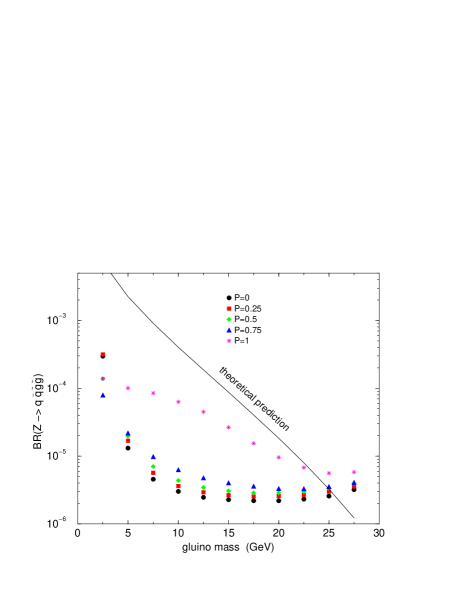
Figure 1: We compare the prediction of $BF(Z\to q\overline{q}\widetilde{g}\widetilde{g})$ compared to the extracted $\!{}^{{\bf?}}$ OPAL 95% CL upper limit as a function of $m_{\widetilde{g}}$ for $P=0,1/4,1/2,3/4,1$. Both smearing and fragmentation effects are included. Results are for the standard $\lambda_{T}$ and $\langle\Delta E\rangle$ (SC1) case. $\!{}^{{\bf?}}$

Figure 2: The cross section (after cuts) in the ${\rm jets}+p\hskip-4.0pt/\hskip 0.0pt_{T}$ channel is compared to (a) the 95% CL upper limit for $L=19~{}{\rm pb}^{-1}$ (which is the same as the $5\sigma$ signal level for $L=100~{}{\rm pb}^{-1}$) at $\sqrt{s}=1.8~{}{\rm TeV}$ and (b) the $S/B=0.2$ level at Run-II ($L\geq 2~{}{\rm fb}^{-1}$, $\sqrt{s}=2~{}{\rm TeV}$) as a function of $m_{\widetilde{g}}$ for $P=1/2$. Standard choices for $\lambda_{T}$ and $\langle\Delta E\rangle$ are employed.

Sample results for OPAL and CDF are illustrated in Figs. 1 and 2. These figures illustrate that, for ‘standard’ choices $\!{}^{{\bf?}}$ of $\lambda_{T}$ and $\langle\Delta E\rangle$, one can use the jets + missing energy OPAL and CDF analyses to exclude any $m_{\widetilde{g}}$ from $\sim 3~{}{\rm GeV}$ up to $\sim 130-150~{}{\rm GeV}$, regardless of the charged fragmentation probability $P$. For $P>1/2$, there is some sensitivity to the $\lambda_{T}$ and $\langle\Delta E\rangle$ scenario choices: limits could be weaker (or stronger). For choices that yield weak limits when $P>1/2$, one can use the OPAL and CDF searches for tracks corresponding to a heavily-ionizing charged particle to eliminate all $m_{\widetilde{g}}$ values up to $\sim 130-150~{}{\rm GeV}$ except in the interval $23\mathrel{\raisebox{-2.58334pt}{$\stackrel{{\scriptstyle\textstyle<}}{{\sim}}$}}m_{\widetilde{g}}\mathrel{\raisebox{-2.58334pt}{$\stackrel{{\scriptstyle\textstyle<}}{{\sim}}$}}50~{}{\rm GeV}$, which is the gap between the OPAL analysis and the current version of the CDF analysis. A refined CDF heavily-ionizing-track analysis should be able to eliminate this gap.

3 Delayed decay signals for gauge-mediated supersymmetry breaking (GMSB)

The two canonical GMSB possibilities are: $\widetilde{\tau}_{R}$=NLSP, with $\widetilde{\tau}_{R}\to\tau\widetilde{G}$; and $\widetilde{\chi}^{0}_{1}=$NLSP followed by $\widetilde{\chi}^{0}_{1}\to\gamma\widetilde{G}$, where the $\widetilde{G}$ is the Goldstino. In either case, the NLSP decay can be either prompt or delayed. In the $\widetilde{\tau}_{R}$-NLSP case, detection of SUSY will be easy, either using heavily ionizing tracks $\!{}^{{\bf?}}$ for long path length of the $\widetilde{\tau}_{R}$ or $\tau$ signals $\!{}^{{\bf?}}$ if the decay is prompt. However, if the $\widetilde{\chi}^{0}_{1}$ is the NLSP, detection of a SUSY signal can be much more challenging, and measurement of the ${\rm SUSY}\hskip-18.0pt/\hskip 13.0pt$ scale, $\sqrt{F}$, requires special attention. $\!{}^{{\bf?}}$ In fact, it is quite possible, and required in some models, that $\sqrt{F}\sim 1000-5000~{}{\rm TeV}$, in which case

$$(c\tau)_{\widetilde{\chi}^{0}_{1}=\widetilde{B}\to\gamma\widetilde{G}}\sim 130\left({100~{}{\rm GeV}\over m_{\widetilde{\chi}^{0}_{1}}}\right)^{5}\left({\sqrt{F}\over 100~{}{\rm TeV}}\right)^{4}\mu{\rm m}$$ (3)

is typically quite large. In particular, in GMSB models with a hidden sector communicating at two-loops with a messenger sector, we have $\!{}^{{\bf?},{\bf?}}$ (to within a factor of 5 or less) $\sqrt{F}>\Lambda\sqrt{f}$, where $f\sim 2.5\times 10^{4}/g_{m}^{4}$ and $\Lambda$ is the parameter that sets the scale of soft-susy-breaking masses. Roughly, $40~{}{\rm TeV}\mathrel{\raisebox{-2.58334pt}{$\stackrel{{\scriptstyle\textstyle<}}{{\sim}}$}}\Lambda\mathrel{\raisebox{-2.58334pt}{$\stackrel{{\scriptstyle\textstyle<}}{{\sim}}$}}150~{}{\rm TeV}$ is required (see below), implying $\sqrt{F}\mathrel{\raisebox{-2.58334pt}{$\stackrel{{\scriptstyle\textstyle>}}{{\sim}}$}}1000-5000~{}{\rm TeV}$. Meanwhile, the gravitino has mass $m_{\widetilde{G}}={F\over\sqrt{3}M_{\rm Planck}}\sim 2.5\left({\sqrt{F}\over 100~{}{\rm TeV}}\right)^{2}~{}{\rm eV}$, and $m_{\widetilde{G}}\mathrel{\raisebox{-2.58334pt}{$\stackrel{{\scriptstyle\textstyle<}}{{\sim}}$}}1$ keV is preferred by cosmology, implying $\sqrt{F}\mathrel{\raisebox{-2.58334pt}{$\stackrel{{\scriptstyle\textstyle<}}{{\sim}}$}}3000~{}{\rm TeV}$. Thus, we should take seriously $1000\mathrel{\raisebox{-2.58334pt}{$\stackrel{{\scriptstyle\textstyle<}}{{\sim}}$}}\sqrt{F}\mathrel{\raisebox{-2.58334pt}{$\stackrel{{\scriptstyle\textstyle<}}{{\sim}}$}}5000~{}{\rm TeV}$ and the possibility of delayed $\widetilde{\chi}^{0}_{1}$ decays. At the very least, one should explore the phenomenology of the model for the full range of possible $\sqrt{F}$ values.

A recent study $\!{}^{{\bf?}}$ has explored Tevatron phenomenology for the full range of $\sqrt{F}$ in a sample model in which the superparticle masses have the relative magnitudes typical of the simpler GMSB models with minimal messenger sector content. In the model employed, the $\widetilde{\chi}^{0}_{1}$ is the LSP and the sparticle masses are: $m_{\widetilde{\chi}^{0}_{1}}\sim 1.35~{}{\rm GeV}\cdot\Lambda$, $m_{\widetilde{\chi}^{+}_{1}}\sim 2.7~{}{\rm GeV}\cdot\Lambda$ ($\sim 2m_{\widetilde{\chi}^{0}_{1}}$), $m_{\widetilde{g}}\sim 8.1~{}{\rm GeV}\cdot\Lambda$ ($\sim 6m_{\widetilde{\chi}^{0}_{1}}$), $m_{\widetilde{\ell}_{R}}\sim 1.7~{}{\rm GeV}\cdot\Lambda$, $m_{\widetilde{\ell}_{L}}\sim 3.5~{}{\rm GeV}\cdot\Lambda$ ($\sim 2m_{\widetilde{\ell}_{R}}$), $m_{\widetilde{q}}\sim 11~{}{\rm GeV}\cdot\Lambda$ ($\sim 6m_{\widetilde{\ell}_{R}}$), with $\Lambda$ in TeV. From these mass formula, we see that if $\Lambda\mathrel{\raisebox{-2.58334pt}{$\stackrel{{\scriptstyle\textstyle<}}{{\sim}}$}}40~{}{\rm TeV}$ then the $\widetilde{\ell}_{R}$ would have been seen at LEP or LEP2, while if $\Lambda\mathrel{\raisebox{-2.58334pt}{$\stackrel{{\scriptstyle\textstyle>}}{{\sim}}$}}150~{}{\rm TeV}$ the $\widetilde{g}$ and the $\widetilde{q}$’s becomes so heavy that naturalness problems for the Higgs sector would certainly be substantial. For the above hierarchy of masses, the primary normal SUSY signal at the Tevatron is the tri-lepton signal. It is found $\!{}^{{\bf?}}$ that this signal is viable for $\Lambda\mathrel{\raisebox{-2.58334pt}{$\stackrel{{\scriptstyle\textstyle<}}{{\sim}}$}}65~{}{\rm TeV}$ for any $\sqrt{F}$; but it does not distinguish a SUGRA-like model from a GMSB model. In order to distinguish between the two model possibilities, one must detect the photon(s) that result from the $\widetilde{\chi}^{0}_{1}$ decays.

One possibility is to detect a prompt photon in association with the tri-lepton signal. One finds that this will be possible only if $\sqrt{F}$ is not very large. Additional associated-photon signals that can be considered include: observation of a photon with non-zero impact-parameter ($b$); decay of the $\widetilde{\chi}^{0}_{1}$ leading to an isolated energy deposit in an outer-hadronic-calorimeter cell (OHC); a photon signal in a specially designed roof-array detector placed on the roof of the detector building (RA); and the appearance of two prompt (emergence before the electromagnetic calorimeter) photons ($2\gamma$). The first three are present only if the $\widetilde{\chi}^{0}_{1}\to\gamma\widetilde{G}$ decay is delayed, while the latter signal will be very weak if the decay is substantially delayed. After imposing strong cuts that hopefully reduce backgrounds to a negligible level (detailed detector studies being needed to confirm), the regions in $(\sqrt{F},\Lambda)$ parameter space for which these signals are viable at the D0 detector for Run-I, Run-II and Tev33 luminosities at the Tevatron are illustrated in Fig. 3.

Figure 3: $\sigma$ contours in the $(\sqrt{F},\Lambda)$ parameter space for the (a) impact-parameter ($b$), (b) outer-hadronic (OHC), (c) roof-array (RA), and (d) prompt-two-photon ($2\gamma$) signals. Contours are given at $\sigma=0.16$, 2.5, and $50~{}{\rm fb}$ — these correspond to 5 events at $L=30,2,0.1~{}{\rm fb}^{-1}$ as for Tev33, Run-II and Run-I, respectively.

We can summarize as follows. If both $\sqrt{F}$ and $\Lambda$ are large, then we will not see either the tri-lepton signal or the prompt $2\gamma$ signal. However, Fig. 3 shows that the large impact parameter photon signal from delayed decays of the $\widetilde{\chi}^{0}_{1}$ can cover most of the preferred parameter space region not accessible by the former two modes. The roof-array detector also provides an excellent signal at large $\sqrt{F}$. Putting all the signals together, the portion of $(\sqrt{F},\Lambda)$ parameter space for which a GMSB $\widetilde{\chi}^{0}_{1}=$NLSP SUSY signal can be seen at the Tevatron is greatly expanded by delayed $\widetilde{\chi}^{0}_{1}$ decay signals. We re-emphasize the fact that one needs the $b$, RA and/or OHC delayed-decay signals to distinguish GMSB from a SUGRA model with GMSB-like boundary conditions when $\sqrt{F}$ is too large for a viable prompt photon signal. Finally, if delayed-decay signatures are seen, an absolutely essential goal will be to determine $\sqrt{F}$ (the most fundamental SUSY parameter of all): the $b$ and RA signals provide the information needed to do so.

4 The nightmare R-parity violating (RPV) scenario

This scenario $\!{}^{{\bf?}}$ is designed as a warning against complacency regarding SUSY discovery. The first ingredient in the nightmare scenario is a non-zero B-violating RPV coupling (often denoted $\lambda^{\prime\prime}$), which leads to LSP decay to three jets: $\widetilde{\chi}^{0}_{1}\to 3j$. This means that the $\widetilde{\chi}^{0}_{1}$’s, resulting from chain decay of a pair of produced supersymmetric particles, do not yield missing energy. The standard jets + $p\hskip-4.0pt/\hskip 0.0pt_{T}$ signal is absent. Of course, for universal gaugino masses at the GUT scale this is not a problem since $m_{\widetilde{\chi}^{\pm}_{1}}\sim 2m_{\widetilde{\chi}^{0}_{1}}$ (at energy scales $<1~{}{\rm TeV}$). For such large $m_{\widetilde{\chi}^{\pm}_{1}}-m_{\widetilde{\chi}^{0}_{1}}$, a robust signal for supersymmetry is provided $\!{}^{{\bf?}}$ by the like-sign dilepton signal that arises when two $\widetilde{\chi}^{+}_{1}$’s (or two $\widetilde{\chi}^{-}_{1}$’s) are produced in the decay chains and both decay leptonically: e.g. $\widetilde{\chi}^{+}_{1}\widetilde{\chi}^{+}_{1}\to\ell^{+}\ell^{+}\nu_{\ell}\nu_{\ell}\widetilde{\chi}^{0}_{1}\widetilde{\chi}^{0}_{1}$. Since the leptons have significant momentum and the neutrinos yield some missing momentum, the like-sign lepton events are typically quite easily isolated at the LHC, and for lower SUSY mass scales, also at the Tevatron. $\!{}^{{\bf?},{\bf?}}$

However, as discussed in an earlier section, if gaugino masses are not universal it is very possible to have $M_{2}<M_{1}\ll|\mu|$ (at energy scales $<1~{}{\rm TeV}$), leading to both $\widetilde{\chi}^{\pm}_{1}$ and $\widetilde{\chi}^{0}_{1}$ being SU(2) winos with $m_{\widetilde{\chi}^{\pm}_{1}}\simeq m_{\widetilde{\chi}^{0}_{1}}$. Also, in the models with $|\mu|\ll M_{1,2}$ the lightest two neutralinos and the lightest chargino are all closely degenerate: $m_{\widetilde{\chi}^{0}_{1}}\simeq m_{\widetilde{\chi}^{\pm}_{1}}\simeq m_{\widetilde{\chi}^{0}_{2}}$. In either case, the leptons in $\widetilde{\chi}^{\pm}_{1}\to\ell^{\pm}\nu\widetilde{\chi}^{0}_{1}$ decays are very soft. The like-sign dilepton signal would be very weak (after necessary cuts requiring reasonable momenta for the leptons). The implications of these scenarios are the following. At LEP2 one would need to use the $e^{+}e^{-}\to\gamma\widetilde{\chi}^{+}_{1}\widetilde{\chi}^{-}_{1}$ photon-tag signal, but, unlike the case where the $\widetilde{\chi}^{0}_{1}$’s from $\widetilde{\chi}^{\pm}_{1}$ decays yield missing energy, the $\widetilde{\chi}^{+}_{1}\widetilde{\chi}^{-}_{1}$ would decay to a final state containing six (relatively soft) jets. Perhaps, such a signal can be shown to be viable over backgrounds up to some reasonable value of $m_{\widetilde{\chi}^{\pm}_{1}}$. To go beyond this value would require a viable signal at the Tevatron and/or LHC. However, at the hadron colliders, leptonic signals will be very weak. Aside from $W$ decays, energetic leptons can emerge only from decays of the heavy gauginos (e.g. the higgsino states in the $M_{2}<M_{1}\ll|\mu|$ case) that are present by virtue of either being directly produced or arising in decays of still heavier produced supersymmetric particles. If the leptonic signals turn out to be too weak, the only signal with a substantial rate will be spherical events containing an extra large number of jets. This signal might prove very difficult to isolate from backgrounds.

5 Two topics regarding Higgs bosons in SUSY.

The first topic concerns the use of experimental limits on the lightest SUSY Higgs boson, $h^{0}$, to exclude parameter regions in various SUSY models. The second topic is the construction of a truly difficult scenario for SUSY (or any) Higgs detection.

5.1 Model constraints from limits on the $h^{0}$

To illustrate the possibilities, I present a brief discussion of two representative papers. The first is that of de Boer et al.. $\!{}^{{\bf?}}$ They assume universal mSUGRA CMSSM (constrained MSSM) boundary conditions and impose radiative electroweak symmetry breaking and gauge coupling unification with $\alpha_{s}(m_{Z})=0.122$ and $m_{t}=173.9\pm 5.2~{}{\rm GeV}$. They also require $b-\tau$ Yukawa unification, with $m_{b}(m_{b})=4.2\pm 0.15~{}{\rm GeV}$ (do we really know it so well?). Additional input data is the current combined ALEPH/CLEO result for $b\to s\gamma$ (including combined errors) and Higgs mass limits from LEP2. Regarding the latter, the CMSSM approach with RGE electroweak symmetry breaking implies that $m_{A^{0}}$ is large and that the $h^{0}$ is very SM-like. Thus, they require $m_{h^{0}}\mathrel{\raisebox{-2.58334pt}{$\stackrel{{\scriptstyle\textstyle>}}{{\sim}}$}}89~{}{\rm GeV}$ at 95% CL. Finally, they require $\Omega h^{2}<1$ for the relic neutralinos of the model. With this input, including a systematic treatment of experimental errors, they compute the $\chi^{2}$ for different parameter choices in the CMSSM context.

They find significant constraints on the allowed parameter space. It is convenient to think of the allowed parameter regions as follows. First, by imposing $b-\tau$ unification they end up with only 4 good $\tan\beta$ and sign($\mu$) solution scenarios: two at low $\tan\beta$ and two at high $\tan\beta$. These 4 possibilities are then restricted by other constraints as shown in the following Table.

Constraint	$\tan\beta=1.65$	$\tan\beta=1.65$
	$\mu<0$	$\mu>0$
$b\to s\gamma$	OK	OK
$m_{h^{0}}>90$?	No	$m_{1/2}>400$
$\Omega h^{2}<1$?	$m_{0}<300$	$m_{0}<300$
Constraint	$\tan\beta=35$	$\tan\beta=64$
	$\mu<0$	$\mu>0$
$b\to s\gamma$	$m_{1/2}>700$	$m_{1/2}>500$
$m_{h^{0}}>90$?	Yes	Yes
$\Omega h^{2}<1$?	$m_{0}>300$	$m_{0}>300$

The Higgs limits are most restrictive for the low-$\tan\beta$ solutions. First, for low $\tan\beta$, $\mu<0$ is pretty much excluded unless one allows $m_{0},m_{1/2}>1~{}{\rm TeV}$. Second, low $\tan\beta$ and $\mu>0$ will soon be excluded if no Higgs is seen at LEP200: for $\mu>0$ and $m_{0},m_{1/2}<1~{}{\rm TeV}$, the other constraints imply $m_{h^{0}}^{\rm max}=97\pm 6~{}{\rm GeV}$ (error dominated by uncertainty in $m_{t}$). If $\tan\beta$ is large, then $m_{h^{0}}^{\rm max}=120\pm 2~{}{\rm GeV}$, which will hopefully be testable at TeV33. The best $\chi^{2}$ solutions have large squark masses $>1~{}{\rm TeV}$ and fine-tuning problems.

Many other studies, especially in the fixed-point context, reach very similar conclusions. For example, Carena et al. $\!{}^{{\bf?}}$ show that $m_{h^{0}}>89~{}{\rm GeV}$ implies a lower bound on $\tan\beta$ well above the perturbativity bound unless the stop mass matrix is carefully chosen. In particular, the fixed-point value of $\tan\beta\sim 1.5$ is allowed only if the heavier stop is not too heavy (i.e. there is an implicit upper bound on $m_{\widetilde{t}_{2}}$). If the bound on $m_{h^{0}}$ increases to $m_{h^{0}}\mathrel{\raisebox{-2.58334pt}{$\stackrel{{\scriptstyle\textstyle>}}{{\sim}}$}}103~{}{\rm GeV}$ (as expected at LEP200), the low-$\tan\beta$ fixed point scenario will be ruled out. Of course, one should keep in mind that the low-$\tan\beta$ fixed point solution is ruled out in mSUGRA and CMSSM if we require $\Omega h^{2}<1$ $\!{}^{{\bf?}}$ and/or no charge/color breaking. $\!{}^{{\bf?}}$ This means, that we can only have a low-$\tan\beta$ fixed-point solution with $m_{h^{0}}>89~{}{\rm GeV}$ that is consistent with $\Omega h^{2}<1$ if we disconnect the slepton, Higgs and squark soft-supersymmetry-breaking mass parameters by not requiring a universal value at the GUT scale. Finally, we recall that adequate electroweak baryogenesis in the MSSM requires $m_{h^{0}}$ in the LEP2 range, a light $\widetilde{t}_{1}$, and small stop mixing. Imposing these constraints in conjunction with the fixed-point low-$\tan\beta$ solution requires $m_{\widetilde{t}_{2}}>2~{}{\rm TeV}$.

Of course, all these constraints depend greatly upon the fact that the MSSM contains exactly two doublets and no other Higgs representations. For example, the constraints found in these studies are obviated if one adds extra singlet(s) $S$ with $\lambda SH_{1}H_{2}$ style coupling.

5.2 A very difficult Higgs scenario: is there a no-lose theorem?

An interesting question that has emerged in several different models is the question of whether there is a no-lose theorem for Higgs discovery at a $\sqrt{s}=500~{}{\rm GeV}$ $e^{+}e^{-}$ collider. Typically, $\!{}^{{\bf?},{\bf?}}$ if one adds just one or two Higgs bosons to the spectrum the answer is yes: one or more of the scalar Higgs bosons will be discovered in the $Zh$ production mode. However, the situation could be much more complicated. A very difficult case $\!{}^{{\bf?}}$ is one in which there are many Higgs bosons, as could arise in a string model with many U(1)’s, $\!{}^{{\bf?}}$ and they share the $ZZ$-Higgs coupling-strength-squared ($g_{ZZh}^{2}$) fairly uniformly. Further, assume these Higgs bosons are spread out such that the experimental resolution is insufficient to resolve the separate peaks, in which case the only signal is an unresolved continuum excess over background. Finally, assume the Higgs bosons all decay into a variety of channels, including invisible decays, various $q\overline{q}$ channels, etc., in which case identification of the $h$ decay final state would not be useful because of the large background in any one channel. In particular, in $e^{+}e^{-}\to Zh$, there would be no guarantee we can use $Z\to q\overline{q}$ or $\nu\overline{\nu}$ decays because of the large number of possible channels in the recoil state and, thus, small signal relative to background in any one channel. The only clearly reliable signal would be an excess in the recoil $M_{X}$ distribution in $e^{+}e^{-}\to ZX$ (with $Z\to e^{+}e^{-}$ and $\mu^{+}\mu^{-}$).

To describe this scenario quantitatively, one $\!{}^{{\bf?}}$ employs a continuum description in which there are Higgs bosons from $m_{h}^{\rm min}$ to $m_{h}^{\rm max}$. Defining $K(m_{h})$ as the $g_{ZZh}^{2}$ strength (relative to SM strength) as a function of $m_{h}$, one then can write two sum rules:

$$\int dm_{h}K(m_{h})\geq 1$$ (4)

$$\int dm_{h}K(m_{h})m_{h}^{2}\leq\langle M^{2}\rangle\,,$$ (5)

where the former becomes an equality if only Higgs singlet and doublet representations are involved. The key to a no-lose theorem is to limit $\langle M^{2}\rangle$. In the context of supersymmetry one can write $\langle M^{2}\rangle\equiv m_{B}^{2}=\lambda v^{2}$, where $v=246~{}{\rm GeV}$ and $\lambda$, a typical quartic Higgs coupling at low energy scales, is limited by requiring perturbativity for $\lambda$ up to some high scale $\Lambda$. In the most general SUSY model, one finds $m_{B}\leq 200~{}{\rm GeV}$ for $\Lambda\sim 10^{17}~{}{\rm GeV}$. Alternatively, independently of a SUSY context, the success of fits to precision electroweak data using $m_{h_{SM}}\mathrel{\raisebox{-2.58334pt}{$\stackrel{{\scriptstyle\textstyle<}}{{\sim}}$}}200~{}{\rm GeV}$ implies, in a multi-Higgs model, that the Higgs bosons with large $K(m_{h})$ must have average mass $\mathrel{\raisebox{-2.58334pt}{$\stackrel{{\scriptstyle\textstyle<}}{{\sim}}$}}200~{}{\rm GeV}$, which would imply $m_{B}\mathrel{\raisebox{-2.58334pt}{$\stackrel{{\scriptstyle\textstyle<}}{{\sim}}$}}200~{}{\rm GeV}$.

Taking $K(m_{h})=K$, a constant, Eq. (4) leads to $K=1/(m_{h}^{\rm max}-m_{h}^{\rm min})$ (assuming only singlet and doublet representations), and Eq. (5) implies

$$m_{B}^{2}\equiv\langle M^{2}\rangle \geq {1\over 3}\left([m_{h}^{\rm max}]^{2}+m_{h}^{\rm max}m_{h}^{\rm min}+[m_{h}^{\rm min}]^{2}\right)\,.$$ (6)

The maximal spread is achieved for $m_{h}^{\rm min}=0$, in which case Eq. (6) requires $m_{h}^{\rm max}\leq\sqrt{3}m_{B}\leq 340~{}{\rm GeV}$.

To analyze this situation, $\!{}^{{\bf?}}$ assume $\sqrt{s}=500~{}{\rm GeV}$, for which $\sigma(Zh)$ for a SM-like $h$ is substantial out to $m_{h}\sim 200~{}{\rm GeV}$. [$\sigma(Zh_{SM})$ falls from $70~{}{\rm fb}$ at low $m_{h}$ to $42~{}{\rm fb}$ at $m_{h}\sim 200~{}{\rm GeV}$.] Confining the signal region to $70\leq m_{h}\leq 200~{}{\rm GeV}$, a fraction $f\sim 0.4$ of the uniform $K(m_{h})$ spectrum would lie in this region. If LEP2 data can eventually be used to show that $K(m_{h})$ is small for $m_{h}\mathrel{\raisebox{-2.58334pt}{$\stackrel{{\scriptstyle\textstyle<}}{{\sim}}$}}70~{}{\rm GeV}$ (i.e. $m_{h}^{\rm min}=70~{}{\rm GeV}$) then $m_{h}^{\rm max}=300~{}{\rm GeV}$ [from Eq. (6) with $m_{B}=200~{}{\rm GeV}$] and a fraction $f\sim 0.55$ would lie in the $70-200~{}{\rm GeV}$ region. Alternatively, one can consider only the $100-200~{}{\rm GeV}$ interval (to avoid the large background in the vicinity of $m_{h}\sim m_{Z}$), in which case $f\sim 0.3$ for $m_{h}^{\rm min}=0$ and $f\sim 0.43$ for $m_{h}^{\rm min}=70~{}{\rm GeV}$, respectively.

The results for the overall excess in $Zh$, with $Z\to e^{+}e^{-}+\mu^{+}\mu^{-}$, integrated over the $70-200~{}{\rm GeV}$ and $100-200~{}{\rm GeV}$ intervals, assuming $\int K(m_{h})=1$ over the interval, are given in Table 2, assuming an integrated luminosity of $L=500~{}{\rm fb}^{-1}$ (which is very optimistic). Including the factor $f$, one finds $S\sim 1350f$ with a background of either $B=6340$ or $B=2700$, for the $70-200~{}{\rm GeV}$ or $100-200~{}{\rm GeV}$ windows, respectively. Correspondingly, one must detect the presence of a broad $\sim 21\%f$ or $\sim 50\%f$ excess over background, respectively. For $f\sim 0.4-0.55$ in the 1st case and $f\sim 0.3-0.43$ in the 2nd case, this would probably be possible. Nominally, $S/\sqrt{B}\sim 17f$ and $\sim 26f$ for the $70-200~{}{\rm GeV}$ and $100-200~{}{\rm GeV}$ windows in $M_{X}$, respectively. However, if $L\mathrel{\raisebox{-2.58334pt}{$\stackrel{{\scriptstyle\textstyle<}}{{\sim}}$}}200~{}{\rm fb}$, the detection of the excess will become quite marginal. As an aside, we note $\!{}^{{\bf?}}$ that $e^{+}e^{-}\to e^{+}e^{-}h$ via $ZZ$-fusion is not useful because of very small $S/B$.

Table 2: Approximate $S$, $B$ and $S/\sqrt{B}$ values for $Zh$ (with $Z\to e^{+}e^{-}+\mu^{+}\mu^{-}$) after integrating the $M_{X}$ recoil mass spectrum from (a) 70 GeV to 200 GeV and (b) 100 GeV to 200 GeV, assuming that many Higgs bosons are distributed evenly throughout the interval with uniform $K(m_{h})$. Results are for $\sqrt{s}=500~{}{\rm GeV}$, $L=500~{}{\rm fb}^{-1}$.

$M_{X}$	$Zh$, $Z\to e^{+}e^{-}+\mu^{+}\mu^{-}$
Interval	$S$	$B$	${S/\sqrt{B}}$
$70-200$	1350	6340	17
$100-200$	1356	2700	26

Table 3: Approximate $S$, $B$ and $S/\sqrt{B}$ values for $Zh$ (with $Z\to e^{+}e^{-}+\mu^{+}\mu^{-}$) in each of the thirteen 10 GeV bins in $M_{X}$ from 70 to 200 GeV, assuming that $S\sim 1350$ events are distributed equally among these bins. We assume $\sqrt{s}=500~{}{\rm GeV}$, $L=500~{}{\rm fb}^{-1}$.

Bin No.	1	2	3	4
$S$	104	104	104	104
$B$	1020	1560	1440	734
$S/\sqrt{B}$	3.3	2.6	2.7	3.8
Bin No.	5	6	7	8–13
$S$	104	104	104	104
$B$	296	162	125	$\sim 130$
$S/\sqrt{B}$	6.0	8.2	9.3	9.1

Of course, if an excess is observed, the next interesting question is whether we can analyze the amount of this excess on a bin-by-bin basis. The situation is illustrated in Table 3 assuming that the roughly 1350 (i.e. $f=1$ for the moment) signal events are distributed equally in the thirteen 10 GeV bins from 70 to 200 GeV. Table 3 gives $S$ for $f=1$, $B$ and the corresponding $S/\sqrt{B}$ value for each bin. Both $S$ and $S/\sqrt{B}$ must be reduced by $f$. One sees that $L=500~{}{\rm fb}^{-1}$ would yield $S/\sqrt{B}>3$ only for the $M_{X}\mathrel{\raisebox{-2.58334pt}{$\stackrel{{\scriptstyle\textstyle>}}{{\sim}}$}}120~{}{\rm GeV}$ bins when $f\sim 0.5$. Further, with only $L=100~{}{\rm fb}^{-1}$ (as might be achieved after a few years of running at a ‘standard’ luminosity design), this bin-by-bin type of analysis would not be possible for 10 GeV bins if $f\sim 0.5$; one really needs $L=500~{}{\rm fb}^{-1}$.

A final question is how many Higgs force us into the continuum scenario? In the inclusive $e^{+}e^{-}\to ZX$ mode, with $Z\to e^{+}e^{-},\mu^{+}\mu^{-}$, the electromagnetic calorimeter and tracking resolutions planned for electrons and muons imply $\Delta m\sim 20~{}{\rm GeV}$ at $\sqrt{s}=500~{}{\rm GeV}$. As a result, something like five Higgs bosons distributed from 70 to 200 GeV would put us into the continuum scenario unless a specific Higgs decay final state (for which resolutions are expected to be below $10~{}{\rm GeV}$ and backgrounds would be smaller) could be shown to be dominant.

6 Doubly-charged Higgs and higgsinos in supersymmetric L-R models

In supersymmetric L-R symmetric models, the Lagrangian cannot contain terms that explicitly violate R-parity. The presence or absence of RPV is determined by whether or not there is spontaneous RPV. There are two generic possibilities. $\!{}^{{\bf?}}$

If certain higher dimensional operators are small or absent, then the scalar field potential must be such that L-R symmetry breaking induces RPV through some combination of non-zero $\langle\widetilde{\nu}^{c}_{i}\rangle$’s. In this case, the $W_{R}$ mass scale is low and, of course, there are lots of new phenomena associated with RPV. In this scenario, the triplet Higgs and higgsinos, including $\Delta^{--}_{L,R}$ and their fermionic partners, are not necessarily light. Considerable phenomenological discussion of the resulting RPV signatures for this case has appeared. $\!{}^{{\bf?}}$

If the above-mentioned higher-dimensional operators are present and are of full strength (but, of course, $\propto 1/M_{U}$ or $1/M_{\rm Planck}$), then L-R symmetry breaking does not require RPV. In this case, the $W_{R}$ mass scale must be very large. Further, the $\Delta_{L}$ triplet members and their superpartners must be very heavy unless one removes the (naturally present) parity-odd singlet from the theory (which is normally included in order to avoid $v_{L}\neq 0$ vacua). However, when the R-sector Higgs mechanism comes in at high scale (assumed to be above the SUSY breaking scale) to give $v_{R}\neq 0$ and generate $W_{R}$ mass, one is breaking a U(3) symmetry and there are 4 surviving massless (goldstone) fields, which are the $\Delta^{--}$ superfield and its charge conjugate, whose component fields only become massive via the higher-dimensional operators. In this case, it is natural for the mass scales of the $\Delta^{--}_{R}$ and $\widetilde{\Delta}^{--}_{R}$, $\sim v_{R}^{2}/M_{\rm Planck}$, to be at the $\sim 100~{}{\rm GeV}$ level.

The phenomenology of doubly charged Higgs bosons has a long history. $\!{}^{{\bf?}}$ The above $\Delta^{--}_{R}$ (hereafter we drop the $R$ subscript) would generally be narrow. Noting that $\Delta^{--}\to W^{-}\Delta^{-}$ is expected to be kinematically forbidden, its primary decay modes would most probably be via the Majorana couplings associated with the see-saw mechanism for neutrino mass generation:

$${\cal L}_{Y}=ih_{ij}\psi^{T}_{i}C\tau_{2}\Delta\psi_{j}+{\rm h.c.}\,,$$ (7)

where $i,j=e,\mu,\tau$ are generation indices, and $\Delta$ is the $2\times 2$ matrix of Higgs fields:

$$\Delta=\pmatrix{\Delta^{+}/\sqrt{2}&\Delta^{++}\cr\Delta^{0}&-\Delta^{+}/\sqrt{2}\cr}\,.$$ (8)

Limits on the $h_{ij}$ by virtue of the $\Delta^{--}\to\ell^{-}\ell^{-}$ couplings include: Bhabbha scattering, $(g-2)_{\mu}$, muonium-antimuonium conversion, and $\mu^{-}\to e^{-}e^{-}e^{+}$. Adopting the convention

$$|h^{\Delta^{--}}_{\ell\ell}|^{2}\equiv c_{\ell\ell}m_{\Delta^{--}}^{2}(~{}{\rm GeV})\,,$$ (9)

one finds $c_{ee}<10^{-5}$ (Bhabbha) and $\sqrt{c_{ee}c_{\mu\mu}}<10^{-7}$ (muonium-antimuonium) are the strongest of the limits. There are no limits on $c_{\tau\tau}$ which is, naively, expected to be the largest. If all the $c$’s are very tiny, virtual versions of $\Delta^{--}\to\Delta^{-}W^{-}$ could be important.

Regarding production, because of the very large $W_{R}$ mass, the doubly-charged Higgs bosons would be primarily produced at hadron colliders via $\gamma^{*},Z^{*}\to\Delta^{--}\Delta^{++}$. At an $e^{-}e^{-}$ or $\mu^{-}\mu^{-}$ collider they could be produced directly as an $s$-channel resonance via the lepton-number-violating couplings $h_{ee}$ and $h_{\mu\mu}$, respectively. The strategy for discovering and studying the $\Delta^{--}$ would be the following. First, one would discover the $\Delta^{--}$ in $p\overline{p}\to\Delta^{--}\Delta^{++}$ with $\Delta^{--}\to\ell^{-}\ell^{-},\Delta^{++}\to\ell^{+}\ell^{+}$ ($\ell=e,\mu,\tau$) at TeV33 or LHC. $\!{}^{{\bf?}}$ One finds that $\Delta^{--}$ detection at the Tevatron ($\sqrt{s}=2~{}{\rm TeV}$, $L=30~{}{\rm fb}^{-1}$) is possible for $m_{\Delta^{--}}$ up to $300~{}{\rm GeV}$ for $\ell=e$ or $\mu$ and up to $180~{}{\rm GeV}$ for $\ell=\tau$. At the LHC, $\Delta^{--}$ discovery is possible up to roughly $925~{}{\rm GeV}$ ($1.1~{}{\rm TeV}$) for $\ell=e,\mu$ and $475~{}{\rm GeV}$ ($600~{}{\rm GeV}$) for $\ell=\tau$, for $L=100~{}{\rm fb}^{-1}$ ($L=300~{}{\rm fb}^{-1}$). Thus, TeV33 + LHC will tell us if such a $\Delta^{--}$ exists in the mass range accessible to the next linear collider or a first muon collider, and, quite possibly, its decays will indicate if it has significant coupling to $e^{-}e^{-}$ and/or $\mu^{-}\mu^{-}$ (unless $\tau^{-}\tau^{-}$ is completely dominant, as is possible). Whether or not these decays are seen, we will wish to determine the strength of these couplings by studying $e^{-}e^{-}$ and $\mu^{-}\mu^{-}$ $s$-channel production of the $\Delta^{--}$. We note that if the $\Delta^{--}$ is observed at the LHC, we will know ahead of time what final state to look in and have a fairly good determination of $m_{\Delta^{--}}$.

At the NLC, taking $L=50~{}{\rm fb}^{-1}$ and defining $R$ to be the beam energy spread in percent,

$$N(\Delta^{--})\sim 3\times 10^{10}\left({c_{ee}\over 10^{-5}}\right)\left({0.2\%\over R}\right)\,,$$ (10)

implying an enormous event rate if $c_{ee}$ is near its upper bound. The ultimate sensitivity to $c_{ee}$ when $\Gamma_{\Delta^{--}}$ is much smaller than the beam energy spread can be estimated by supposing that 100 events are required. From Eq. (10), we predict 100 $\Delta^{--}$ events for

$$\left.c_{ee}\right|_{\rm 100~{}events}\sim 3.3\times 10^{-14}(R/0.2\%)\,,$$ (11)

independent of $m_{\Delta^{--}}$, which is dramatic sensitivity. Because of the much smaller $R$ values possible at a $\mu^{-}\mu^{-}$ collider ($R\sim 0.003\%$ is possible), comparable or greater sensitivity to $c_{\mu\mu}$ could be achieved there despite the lower expected integrated luminosity.

In the L-R symmetric models the phenomenology of the doubly-charged Higgsinos would be equally interesting. $\!{}^{{\bf?}}$ The basic experimental signatures always involve $\tau$’s. In non-GMSB SUSY, if $h_{\tau\tau}$ is full strength ($\sim 0.5$) then it influences the RGE’s so that the $\widetilde{\tau}$’s (especially $\widetilde{\tau}_{R}$) are lighter than $\widetilde{e}$ and $\widetilde{\mu}$, even if $\tan\beta$ is not large. Further, starting with a common mass at the $v_{R}$ scale, evolution leads to $m_{\Delta^{--}}<m_{\widetilde{\Delta}^{--}}$ and the $\Delta^{--}$ would be easily visible as described above. Less attention has been paid to $\widetilde{\Delta}^{--},\widetilde{\Delta}^{++}$, which could be produced at the Tevatron in pairs. Indeed, for $m_{\Delta^{--}}=m_{\widetilde{\Delta}^{--}}$, the $\widetilde{\Delta}^{--}\widetilde{\Delta}^{++}$ pair cross section is bigger than that for $\Delta^{--}\Delta^{++}$ due to the fact that the former is not $p$-wave suppressed. Normally, $\widetilde{\Delta}^{--}\to\widetilde{\tau}_{R}\tau$ is kinematically allowed and will dominate over all other lepton channels because of larger coupling. The dominant $\widetilde{\tau}_{R}$ decay would be $\widetilde{\tau}_{R}\to\widetilde{\chi}^{0}_{1}\tau$. Thus, a typical signature would be $p\overline{p}\to\widetilde{\Delta}^{--}\widetilde{\Delta}^{++}\to\tau^{-}\tau^{-}\tau^{+}\tau^{+}+p\hskip-4.0pt/\hskip 0.0pt_{T}$. Note that the presence of $p\hskip-4.0pt/\hskip 0.0pt_{T}$ would make reconstruction of the $\Delta^{--}$ and $\Delta^{++}$ masses difficult.

In the GMSB context there are some alterations to the above scenario. First, one finds that the $\widetilde{\Delta}^{--}$ is now lighter than the $\Delta^{--}$. In fact, the $\widetilde{\Delta}^{--}$ could even be the NLSP. If not, the $\widetilde{\tau}_{R}$ very probably is (even for minimal messenger sector content), with $\widetilde{\tau}_{R}\to\tau\widetilde{G}$ being its dominant decay. The typical signature would be the same as above except the $p\hskip-4.0pt/\hskip 0.0pt_{T}$ would now be due to the $\widetilde{G}$’s rather than $\widetilde{\chi}^{0}_{1}$’s. In the small portion of parameter space where the $\widetilde{\chi}^{0}_{1}$ is the NLSP, the signature for $\widetilde{\Delta}^{--}\widetilde{\Delta}^{++}$ production changes to $4\tau 2\gamma+p\hskip-4.0pt/\hskip 0.0pt_{T}$, where the $\gamma$’s come from the $\widetilde{\chi}^{0}_{1}\to\gamma\widetilde{G}$ decays.

Overall, a supersymmetric L-R symmetric model would give rise to a very unique phenomenology with many exciting ways to explore the content and parameters of the model.

7 Conclusion

I have tried to give an overview of recent results in supersymmetry phenomenology with emphasis on unusual scenarios that one might encounter, especially ones for which detection of supersymmetric particles and/or the SUSY Higgs bosons might require special experimental/analysis techniques. Experimentalists should pay attention to these special cases to make sure that their detector designs, triggering algorithms and analysis techniques do not discard these possibly important signals.

References

References

- [1] The phenomenology is discussed in C.H. Chen, M. Drees and J.F. Gunion, Phys. Rev. Lett. 76, 200 (1996); Phys. Rev. D 55, 330 (1997).
- [2] G. Anderson, C.H. Chen, J.F. Gunion, J. Lykken, T. Moroi, Y. Yamada, in New Directions for High-Energy Physics, Proceedings of the 1996 DPF/DPB Summer Study on High Energy Physics, Snowmass ’96, edited by D.G. Cassel, L.T. Gennari and R.H. Siemann (Stanford Linear Accelerator Center, Stanford, CA, 1997) pp. 669–673, hep-ph/9609457.
- [3] DELPHI Collaboration, http://delphiwww.cern.ch/delfig/figures/search/chadeg172/char_dege.html.
- [4] A. de Gouvea, A. Friedland and H. Murayama, hep-ph/9803481.
- [5] H. Baer, C.H. Chen and X. Tata, Phys. Rev. D 35, 075008 (1998).
- [6] This is exemplified by the work of T. Ibrahim and P. Nath, hep-ph/9807501, in the ‘mSUGRA’ context.
- [7] M. Brhlik and G. Kane, hep-ph/9803391.
- [8] S. Raby, Phys. Rev. D 56, 2852 (1997); Phys. Lett. B 422, 158 (1998); S. Raby and K. Tobe, hep-ph/9807281.
- [9] H. Baer, K. Cheung and J.F. Gunion, hep-ph/9806361.
- [10] J.F. Gunion and D. Soper, Phys. Rev. D 15, 2617 (1977).
- [11] J. Feng and T. Moroi, Phys. Rev. D 58, 035001 (1998).
- [12] B. Dutta, D.J. Muller and S. Nandi, hep-ph/9807390; K. Cheung and D. Dicus, Phys. Rev. D 58, 057705 (1998).
- [13] C.-H. Chen and J.F. Gunion, Phys. Lett. B 420, 77 (1998) and Phys. Rev. D 58, 075005 (1998).
- [14] J.F. Gunion, in Future High Energy Colliders, Proceedings of the ITP Symposium, U.C. Santa Barbara, October 21–25, 1996, AIP Press, ed. Z. Parsa, pp. 41–64.
- [15] A. de Gouvea, T. Moroi and H. Murayama, Phys. Rev. D 56, 1281 (1997).
- [16] J.F. Gunion, under study.
- [17] P. Binetruy and J.F. Gunion, in Heavy Flavors and High Energy Collisions in the 1—100 TeV Range, Proceedings of the INFN Eloisatron Project Workshop, Erice, Italy, June 10–27, 1988, edited by A. Ali and L. Cifarelli (Plenum Press, New York, 1989) p. 489.
- [18] H. Dreiner and G.G. Ross, Nucl. Phys. B 365, 597 (1991); H. Dreiner, M. Guchait and D.P. Roy, Phys. Rev. D 49, 3270 (1994); V. Barger, M.S. Berger, P. Ohmann, R.J.N. Phillips, Phys. Rev. D 50, 4299 (1994); H. Baer, C. Kao and X. Tata, Phys. Rev. D 51, 2180 (1995); H. Baer, C.-H. Chen and X. Tata, Phys. Rev. D 55, 1466 (1997); A. Bartl et al., Nucl. Phys. B 502, 19 (1997).
- [19] Example: W. de Boer et al., hep-ph/9805378.
- [20] M. Carena, P. Chankowski, S. Pokorski and C. Wagner, hep-ph/9805349.
- [21] J. Ellis, T. Falk, K. Olive and M. Schmitt, Phys. Lett. B 413, 355 (1977).
- [22] S.A. Abel and B.C. Allanach, Phys. Lett. B 431, 339 (1998).
- [23] J. Kamoshita, Y. Okada and M. Tanaka, Phys. Lett. B328 67 1994 ; B.R. Kim, S.K. Oh and A. Stephan, Proceedings of the 2nd International Workshop on “Physics and Experiments with Linear Colliders”, edited by F. Harris, S. Olsen, S. Pakvasa and X. Tata, Waikoloa, HI, (World Scientific, Singapore, 1993) p. 860; B.R. Kim, G. Kreyerhoff and S.K. Oh, hep-ph/9711372.
- [24] J.R. Espinosa and J.F. Gunion, hep-ph/9807275.
- [25] K.R. Dienes, Phys. Rep. 287, 447 (1997).
- [26] See, for example, K. Kuchimanchi and R.N. Mohapatra, Phys. Rev. Lett. 75, 3989 (1995); and Z. Chacko and R.N. Mohapatra, Phys. Rev. D 58, 015001 (1998).
- [27] For a brief review and references, see K. Huitu, J. Maalampi and K. Puolamaki, hep-ph/9708491, in Proceedings of the 5th International Conference on Physics Beyond the Standard Model, Balholm, Norway, 1997, p. 500.
- [28] J.F. Gunion, Int. J. Mod. Phys. A 11, 1551 (1996) and Int. J. Mod. Phys. A 13, 2277 (1998).
- [29] J.F. Gunion, C. Loomis and K. Pitts, in New Directions for High-Energy Physics, Proceedings of the 1996 DPF/DPB Summer Study on High Energy Physics, Snowmass ’96, edited by D.G. Cassel, L.T. Gennari and R.H. Siemann (Stanford Linear Accelerator Center, Stanford, CA, 1997) p. 603, hep-ph/9610237.
- [30] B. Dutta and R. Mohapatra, hep-ph/9804277.