TMU-HEL-9807
hep-ph/9810387
Current Status of the Solar Neutrino Problem with Super-Kamiokande

Abstract

We perform an updated model-independent analysis using the latest solar neutrino data obtained by ³⁷Cl and ⁷¹Ga radiochemical experiments, and most notably by a large water-Cherenkov detector SuperKamiokande with their 504 days of data taking. We confirm that the astrophysical solutions to the solar neutrino problem are extremely disfavored by the data and a low-temperature modification of the standard solar model is excluded by more than 5 $\sigma$. We also propose a new way of illuminating the suppression pattern of various solar neutrino flux without invoking detailed flavor conversion mechanisms. It indicates that the strong suppression of ⁷Be neutrinos is no more true when the neutrino flavor conversion is taken into account.

I Introduction

The existence of the solar neutrino problem [1, 2] is now established more or less independently of any details of solar models. It was first recognized by Bahcall and Bethe [3] that the observed rate in the ³⁷Cl experiment [4] is lower than the lower limit imposed by the ⁸B neutrino flux observed in the Kamiokande experiment [5]. The similar argument has been repeated [6, 7] with the ⁷¹Ga experiments [8, 9]. The outcome of these analyses can be phrased as the “missing ⁷Be neutrinos” because there left little room for ⁷Be neutrinos.

The analysis has been made more systematic by a series of works that is categorized now as the “model-independent analysis”. This type of analysis was first attempted by Spiro and Vignaud [10] and was established by Hata, Bludman and Langacker [11]. In both works the first use is made of the luminosity constraint which will be reviewed in Appendix. An incomplete list of the subsequent relevant references are given in [12, 6, 13, 14, 15, 16, 17]. The type of analysis was further refined by many people; Hata et al. [11, 14] and Parke [15] used the luminosity constraint to obtain the allowed region on two-dimensional (e.g., ⁷Be $-$ ⁸B flux) plane. Then, the most elaborated version of the luminosity constraint was formulated by Bahcall and Krastev [16] who also obtained a parameter-independent constraint on various neutrino flux within the MSW [18] as well as the just so solutions [19] of the solar neutrino problem. A detailed model-independent analysis without the luminosity constraint which also includes the effects of the $pep$ and the CNO neutrinos was carried out by Heeger and Robertson [17].

The most important message from these model-independent analyses is that the solar neutrino problem cannot be accounted for by astrophysical mechanisms unless some assumptions in the standard electroweak theory or solar neutrino experiments are grossly incorrect.

In this paper, we update the model-independent analysis of the solar neutrino problem by including the newest data of the high-statistics water Cherenkov detector, SuperKamiokande [20, 21], as well as those of the latest ³⁷Cl [4] and the ⁷¹Ga experiments [8, 9]. We also use the new values of the expected event rates in the solar neutrino experiments obtained in the latest standard solar model (SSM) calculation by Bahcall and Pinsonneault (BP98) [22] which was made available quite recently. Our analysis will indicate that sensible astrophysical modifications of the solar model such as the low-temperature ($T$) model [1] is convincingly excluded by the present data.

We also try to develop a new method for illuminating the suppression pattern of various solar neutrino flux originated from different fusion reactions in a less model-dependent fashion. It is aimed to bridge between the aforementioned model-independent analysis and the detailed analyses [16, 23, 24, 25, 26, 27, 28, 29] of the solar neutrino data based on the particular neutrino flavor conversion mechanisms such as the MSW mechanism or the just-so solution. We will observe that the statement of the missing ⁷Be neutrinos is no more true in the presense of neutrino flavor conversion.

II The Data

TABLE I.: Observed solar neutrino event rates used in this analysis and corresponding predictions from the reference standard solar model [22]. The quoted errors are at $1\sigma$.

Experiment	Data $\pm$(stat.) $\pm$(syst.)	Ref.	Theory [22]	Units
Homestake	$2.56\pm 0.16\pm 0.15$	[4]	$7.7^{+1.2}_{-1.0}$	SNU
SAGE	$69.9^{+8.0}_{-7.7}{}^{+3.9}_{-4.1}$	[8]	$129^{+8}_{-6}$	SNU
GALLEX	$76.4\pm 6.3^{+4.5}_{-4.9}$	[9]	$129^{+8}_{-6}$	SNU
SuperKam	$2.44\pm 0.05{}^{+0.09}_{-0.07}$	[21]	$5.15^{+0.98}_{-0.72}$	$10^{6}$ cm-2s-1

We tabulate in Table 1 the latest solar neutrino data which we will use in our analysis in this paper. The table includes the ⁸B neutrino flux measured during 504 days in the SuperKamiokande experiment [21] (assuming the conventional $\beta$ decay spectrum of ⁸B neutrinos). In the present analysis we will use only the SuperKamiokande data without including the Kamiokande data because of the larger statistics and the smaller systematic error in the SuperKamiokande.

Our analysis in the present work is based only upon the total rate of each experiment, and the information of the energy spectrum of ⁸B neutrinos, which is made available by the water Cherenkov experiments, is not taken into account. Therefore, it is to illuminate the global features of the suppression of the solar neutrino spectrum. We hope that this analysis is complementary with the ones that constrain allowed parameter regions in a stringent way with such full informations and by using the particular mechanism of flavor transformation, e.g., the MSW mechanism.

For the purpose of our analysis we assume that the statistical and the systematic errors are independent with each other so that they can be combined quadratically. We found, from the values presented in Table I,

$$S^{obs}_{Cl} = 2.56\pm 0.23\ \ \ \mbox{SNU},$$ (1)

$$S^{obs}_{Ga} = 72.4\pm 6.6\ \ \ \mbox{SNU},$$ (2)

$$S^{obs}_{SK} = (2.44\pm 0.10)\ \times\ 10^{6}\ \mbox{cm}^{-2}\mbox{s},$$ (3)

where, to be conservative, we always take the larger values of statistical and systematic errors, whenever errors are asymmetric, in each experiment before we combine.

The number for ${}^{71}\mbox{Ga}$ experiment, however, requires some comments. In order to determine the combined central value, we first combine the statistical and the systematic errors quadratically in each experiment, and then take the weighted average of SAGE [8] and GALLEX [9] results following the method described in [30]. The associated error for the combined (central) value for the ⁷¹Ga  experiment is determined by the following equation,

$$\sigma^{obs}_{Ga}\equiv\sqrt{\sigma_{stat}^{2}+\sigma_{syst}^{2}}$$ (4)

where

$$\sigma_{stat}=\left[\sum_{i}\frac{1}{(\sigma_{stat}^{i})^{2}}\right]^{-1/2}$$ (5)

and we take the largest value, 4.7 SNU, among the systematic errors in GALLEX and SAGE, for $\sigma_{syst}$ in Eq. (4).

Sometimes we need in our analysis the ratios of these experimental values to the expected ones by the SSM. If we use the latest standard solar model calculation by Bahcall and Pinsonneault (BP98) [22], the ratio for the SuperKamiokande is given as,

$$R^{obs}_{SK}\equiv\frac{\Phi^{obs}_{SK}(^{8}\mbox{B})}{\Phi^{SSM}(^{8}\mbox{B})}=\frac{2.44\pm 0.11}{5.15}\simeq 0.47\pm 0.021,$$ (6)

where we used the central value of BP98 in the denominator of (6). Hereafter, we always take the flux values and the event rate given in BP98 as reference values of SSM.

III Model-Independent Analysis

In this section we perform model-independent analysis of the solar neutrino data.

A fundamental assumptions

The fundamental assumption behind the analyses in this paper is as follows:

(i) The sun shines due to the nuclear fusion reactions from which and only from which the solar neutrinos come.

(ii) The relevant reactions which are responsible for generating neutrinos in the sun are assumed to be those postulated in the SSM.

(iii) The sun is quasi-stable during the time scale of 0.1-1 million years, an order of magnitude of time difference between those required to neutrinos and photons to exit the sun after created at its central part.

These assumptions allows us to relate the solar neutrino flux to the present solar luminosity. Note, however, that we will discuss in Sec. IV the case in which this constraint effectively does not apply.

As will be described in detail in Appendix the fundamental assumptions (i) to (iii) given in Sec.I imply that the solar neutrino flux generated by various nuclear fusion reactions must obey the luminosity constraint [10, 11, 15, 16],

$$\frac{L_{\odot}}{4\pi R^{2}}=\sum_{\alpha}\left(\frac{Q}{2}-\left\langle E\right\rangle_{\alpha}\right)\Phi(\alpha)$$ (7)

where $R$ = 1 A.U. ($1.469\times 10^{13}$ cm), $\left\langle E\right\rangle_{\alpha}$ and $\Phi(\alpha)$ ($\alpha=pp$, ⁷Be, ⁸B,…) denote the average energy loss by neutrinos and the neutrino flux, respectively.

We normalize the neutrino flux to those of the SSM of BP98 [22] in this work and define fractional flux $\phi^{\alpha}$ as

$$\phi^{\alpha}=\frac{\Phi(\alpha)}{\Phi(\alpha)_{SSM}},\ \ (\alpha=pp,^{7}\mbox{Be},^{8}\mbox{B},...)$$ (8)

where

$$\Phi(pp)_{SSM} = 5.94\times 10^{10}\ \ \mbox{cm}^{-2}\mbox{sec}^{-1},$$ (9)

$$\Phi(^{7}\mbox{Be})_{SSM} = 4.80\times 10^{9}\ \ \mbox{cm}^{-2}\mbox{sec}^{-1},$$ (10)

$$\Phi(^{8}\mbox{B})_{SSM} = 5.15\times 10^{6}\ \ \mbox{cm}^{-2}\mbox{sec}^{-1}.$$ (11)

Using these numbers the luminosity constraint is simply given by,

$$1=0.907\phi^{pp}+0.0755\phi^{{}^{7}Be}+4.97\times 10^{-5}\phi^{{}^{8}B},$$ (12)

where we used the value, $L_{\odot}=3.844\times 10^{33}$ (erg/s) [31]. The reason why the right hand side of Eq. (12) does not give unity for the SSM flux (for all $\phi^{i}=1$) is that we have neglected the contribution from CNO and $pep$ neutrinos.

In this section we make the following more specific assumptions (1) and (2) in addition to the fundamental assumptions (i) - (iii):

(1) The energy spectra of the solar neutrinos are not modulated.

(2) Neutrino flavor transformation does not occur inside the sun and the earth, as well as in the space between the sun and the earth.

It follows from these two assumptions that the luminosity constraint is effective, and the flux $\Phi$ is the real flux to be detected by the terrestrial detectors. The basic physical picture of the cases we try to test in this section are the astrophysical solution of the solar neutrino problem, such as the low-temperature model of the solar core. Once particle physics mechanisms beyond the standard electroweak theory are involved, generally speaking, the shape of the solar neutrino energy spectra can be altered from those predicted by the SSM.

B analysis

The expected solar neutrino signal to the ³⁷Cl, ⁷¹Ga and SuperKamiokande solar neutrino experiments are given in terms of neutrino flux by,

$$S^{th}_{Cl} = 5.9\phi^{{}^{8}B}+1.15\phi^{{}^{7}Be}\ \ \ \mbox{SNU},$$ (13)

$$S^{th}_{Ga} = 12.4\phi^{{}^{8}B}+34.4\phi^{{}^{7}Be}+69.6\phi^{pp}\ \ \ \ \mbox{SNU},$$ (14)

$$R^{th}_{SK} = \phi^{{}^{8}B},$$ (15)

where we have neglected the contribution from the $pep$ and the CNO neutrinos. We believe that inclusion of them does not affect our conclusion in this section, because the results barely change unless their flux is extremely large compared with those predicted by SSM.

Using Eqs. (13-14) as well as the observed solar neutrino data summarized in Table I we perform a simple $\chi^{2}$ analysis. We used the luminosity constraint (12) to eliminate $\phi^{pp}$ in favor of $\phi^{{}^{7}Be}$ and $\phi^{{}^{8}B}$. We then freely vary the two flux, $\phi^{{}^{8}B}$ and $\phi^{{}^{7}Be}$. Since the minimum $\chi^{2}$ is reached when $\phi^{{}^{7}Be}$ takes a negative value as in the previous analyses we impose the condition $\phi^{{}^{7}Be}\geq 0$ because the flux must be positive.

FIG. 1.: Contour plot of the $\chi^{2}$ values in the $\Phi_{{}^{8}B}-\Phi_{{}^{7}Be}$ plane for different combinations of the solar neutrino experiments. The solid curves correspond to 1 $\sigma$ to 5 $\sigma$, with step size 1, from inside to outside. We also indicate the 1,2 and 3 $\sigma$ theoretical range predicted by BP98, by the solid, dotted and dashed lines, respectively. Along the dashed curve, $\phi^{{}^{7}Be}=(\phi^{{}^{8}B})^{10/24}$, the crosses indicate, from left to right, the point where the central temperatures are 0.85, 0.9,0.95,0.98,1 and 1.01 with respect to the prediction by the SSM.

We plot in Figs. 1 the contours of $\chi^{2}\equiv\chi^{2}_{min}+\Delta\chi^{2}$ where $\Delta\chi^{2}$ = 2.3, 6.2, 11.8, 19.4 and 28.7, correspond to 1$\sigma$, 2$\sigma$, … 5 $\sigma$, respectively, for two free parameters. In Fig. 1 also plotted is the curve $\phi^{{}^{7}Be}=(\phi^{{}^{8}B})^{10/24}$ which corresponds to the case where the central temperature of the sun $T_{c}$ is varied freely. There is a relationship between the two flux as represented by the curve because of approximate power-law dependences of the flux [32],

$$\phi^{{}^{7}Be} \propto T_{c}^{10}$$ (16)

$$\phi^{{}^{8}B} \propto T_{c}^{24},$$ (17)

hence, the power law relation as indicated in Fig. 1 . (Note that the flux $\Phi(\alpha)_{SSM}$ in the denominator of (8) is the BP98 flux with the fixed temperature predicted by the SSM. We hope that no confusion arises.) We also note that additional flux constraint in Eq. (9) in ref. [16] is obeyed.

As in the previous analyses [11, 12, 6, 13, 14, 15, 16, 17] the minimum $\chi^{2}$ is achieved by vanishing ⁷Be flux. It is true not only in Fig. 1 (a) where all the ³⁷Cl , ⁷¹Ga  , and SuperKamiokande data are taken into account, but is also true in Fig. 1 (b-d) where only two of them are analyzed. It is obvious, by comparing Fig. 1 (a) with those of [11] and by [15], or by comparing Figs. 1 (b),(d) with Fig. 1 (c), that widths of the contours have been greatly shrunk along the $\phi^{{}^{8}B}$ axis. This is a clear indication of how strongly the analysis is affected by the high statistics data from SuperKamiokande.

From Fig. 1 we conclude that the standard solar model is strongly in disagreement with the data as was also concluded recently in ref. [33]. We can see from Fig. 1 that BP98 SSM is ruled out by the current solar neutrino data at the significance level much higher than 5$\sigma$ under our fundamental assumptions (i)-(iii) and the additional ones (1)-(2). We have confirmed that the astrophysical solution of the solar neutrino problem is strongly disfavored by the data. In particular, the low-$T$ model is excluded by a confidence level more than 5 $\sigma$. This is the level at which one can safely claim that the hypothesis is rejected [30]. It is also clear from Figs. 2-4 that removing one of the three types of the solar neutrino experiments cannot save the SSM. The low-$T$ model is still excluded by confidence levels of more than 3 $\sigma$.

IV Suppression Pattern of Neutrino Flux implied by the current Solar Neutrino Data

In this section we describe a new way of illustrating the suppression pattern of neutrino flux from major nuclear reactions in the sun that is required to explain the current solar neutrino experiments. We do this by taking into account the possibility that $\nu_{e}$’s produced in the solar core are converted into either different flavor active neutrinos ($\nu_{\mu}$ and/or $\nu_{\tau}$) or sterile ones $\nu_{s}$ in their journey to the terrestrial detectors.

To obtain global understanding of the suppression pattern we propose to combine the $pep$ and the CNO neutrinos into the ⁷Be neutrinos and denote them as the intermediate energy neutrinos. In the context of the model-independent analysis performed in Sec.III it is more reasonable to combine the $pep$ neutrinos with the ${pp}$’s because they are competing partners in the ${pp}$ I chain reaction. But, here we are interested in knowing the preferred suppression pattern and it is more conceivable to combine the flux when their energy regions overlap.

Therefore, we try to determine the reduction rate of the flux of low energy ${pp}$ neutrinos, intermediate energy ⁷Be+CNO+$pep$ neutrinos, and the high energy ⁸B neutrinos at the earth by adjusting their survival probabilities such that the experimental data can be fitted. Since the luminosity constraint is not very effective with neutrino flavor transformations we disregard it in this section.

We assume, in this section (except in Subsec. IV.C), that neutrino production rates from each source are the same as the ones predicted by the BP98 SSM. Then the expected signal in each experiment in the presence of neutrino conversion, $\nu_{e}\to\nu_{\mu,\tau}$, is given by,

$$S^{th}_{Cl} = 5.9\langle{P_{B}}\rangle+1.83\langle{P_{I}}\rangle\ \ \ \mbox{SNU},$$ (18)

$$S^{th}_{Ga} = 12.4\langle{P_{B}}\rangle+46.9\langle{P_{I}}\rangle+69.6\langle{P_{pp}}\rangle\ \ \ \ \mbox{SNU},$$ (19)

$$R^{th}_{SK} = \langle{P_{B}}\rangle+r(1-\langle{P_{B}}\rangle),$$ (20)

where $\langle{P_{B}}\rangle$, $\langle{P_{I}}\rangle$ and $\langle{P_{pp}}\rangle$ are the average survival probabilities for ⁸B, intermediate energy and $pp$ neutrinos, respectively. The symbol $\langle...\rangle$ has to be regarded as the average over the neutrino flux times the cross section, and as well as the detection efficiency in the case of the SuperKamiokande experiment. In Eq. (20) $r$ is essentially given by the ratio of the scattering cross section of $\nu_{\mu(\tau)}$ to that of $\nu_{e}$ off electron,

$$r\equiv\frac{\langle\sigma_{\nu_{\mu}e}\rangle}{\left\langle\sigma_{\nu_{e}e}\right\rangle}\simeq 0.16,$$ (21)

where the cross sections are averaged over by the SSM ⁸B neutrino spectrum multiplied by the SuperKamiokande detection efficiency as adopted in ref. [34]. When we consider (in Subsec. IV.B) the case where the ⁸B $\nu_{e}$’s are converted into some sterile state, we will drop the 2nd term in (20).

In eqs. (18-20) we simply assume that the average survival probability for all the intermediate energy $pep$, CNO and ⁷Be neutrinos are the same and denoted it as $\langle{P_{I}}\rangle$ so that the coefficient of $\langle{P_{I}}\rangle$ in eqs. (18) and (19) now includes the contribution not only from ⁷Be but also from $pep$ and CNO neutrinos (cf. eqs. (13) and (14)). Furthermore, we take, as an approximation, $\langle{P_{i}}\rangle$ ($i=$ $pp$, $I$, ⁸B) to be equal for all the experiments despite the fact that, in general, the neutrino conversion can distort the neutrino energy spectra, and therefore, $\langle{P_{i}}\rangle$ can be different depending upon experiments. Such an approximation is reasonable because the energy dependences of the flux times cross section (times the detection efficiency for the SuperKamiokande) are rather similar among different experiments, as first noticed by Kwong and Rosen [13].

Other than these assumptions, we do not consider any specific mechanism of neutrino flavor transformation in this analysis but aim at illuminating global features of the modification of the solar neutrino spectrum. In this sense it is complementary with thorough analyses based on the MSW mechanism [23, 24, 16, 26, 27, 28, 29], or the vacuum oscillation [25, 16].

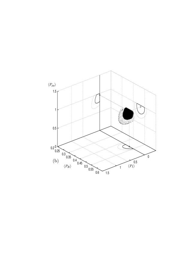
FIG. 2.: Allowed range of neutrino flux determined by all the solar neutrino experiments with the condition $\chi^{2}=\chi^{2}_{min}+\Delta\chi^{2}$ where $\Delta\chi^{2}$ = 3.5 (1$\sigma$) and 8.0 (2$\sigma$) (for three free parameters) assuming the neutrino conversion (a) $\nu_{e}\to\nu_{\mu,\tau}$ and (b) $\nu_{e}\to\nu_{s}$. The allowed ranges are projected into each plane, indicated by the solid curves (1$\sigma$) and the dotted curves (2$\sigma$). The best fitted reduction rates of the neutrino fluxes are, ($\langle P_{B}\rangle$, $\langle P_{I}\rangle$, $\langle P_{pp}\rangle$) = (0.37, 0.19, 0.84) with $\chi^{2}_{min}\sim 0$ for the active conversion and =(0.47, 0, 0.96) $\chi^{2}_{min}\sim 0.8$ for the sterile conversion.

A The case of active neutrinos

We present our results in Fig. 2 (a) for the case of active conversion. We note that $\langle P_{B}\rangle$ is determined most accurately, as is expected from the large statistics of the SuperKamiokande experiment. On the other hand, the other two, $\langle P_{I}\rangle$ and $\langle P_{pp}\rangle$, have larger uncertainties at the present stage of the solar neutrino data. We also tabulate the range of allowed values of the survival probabilities with their 1 $\sigma$ uncertainties in Table 2.

From Fig. 2 (a) and Table 2 we can see that strong suppression of intermediate energy neutrinos, the one best fit by negative flux, is no more true when the neutrino flavor conversion is taken into account. This feature is in sharp contrast with the results of the model-independent analysis in Sec.III and of the flavor conversion into sterile neutrinos to be discussed below.

TABLE II.: The range of reduction rates of each neutrino flux with respect to the prediction by BP98 SSM implied by the solar neutrino data. We present the both cases with (a) and without (b) pep and CNO contribution.

Case	$\langle P_{B}\rangle$	$\langle P_{I}\rangle$	$\langle P_{pp}\rangle$
Active (a)	$0.33-0.42$	$0-0.46$	$0.6-1$
Active (b)	$0.33-0.42$	$0-0.74$	$0.55-1$
Sterile (a)	$0.43-0.50$	$0-0.16$	$0.77-1$
Sterile (b)	$0.43-0.50$	$0-0.26$	$0.76-1$

We stress that the proposed experiments such as Borexino [35], Hellaz [36] and Heron [37] are needed in order to determine the ⁷Be and $pp$ neutrino flux with smaller uncertainties, especially when the conversion mechanism is not unknown. For example, once ⁷Be neutrino flux is determined by Borexino then the $pp$ neutrino flux would also be well determined by combining the results of the other solar neutrino experiments and vice versa.

We also mention that the suppression rate of the intermediate-energy neutrinos depends rather sensitively on the presense or absence of the $pep$ and CNO neutrinos. If we ignore their contribution the best fit value of $\langle P_{I}\rangle$ (=$\langle P_{Be}\rangle$) becomes larger by a factor of 2 (see Table II).

B The case of sterile neutrinos

We next consider the case where the neutrinos are converted into sterile species. Since only the water-Cherenkov experiment can be sensitive to the difference between conversions into active and sterile neutrinos any change in our result from the active case solely comes from ⁸B neutrinos. The results for the sterile neutrino conversion is presented in Fig. 2 (b) and in Table 2. By comparing Fig. 2 (a) and (b), we can clearly see that the stronger suppression of ⁷Be neutrinos is required than in the case of active conversion with unsuppressed ⁸B flux, $\phi^{{}^{8}B}=1$. We note that the best fit is obtained when the flux of intermediate energy neutrino is negative. One can interpretate Fig. 2 (b) as presenting in a novel style of 3 dimensional plot the updated result of the model-independent analysis without the luminosity constraint [17]. From this viewpoint our result indicates that the feature of strong suppression of ⁷Be neutrinos is insensitive to switching on and off the luminosity constraint.

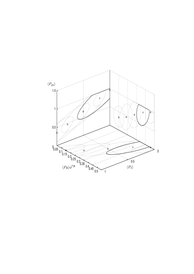
FIG. 3.: Two sigma allowed range of neutrino flux, projected into each plane, assuming the neutrino conversion $\nu_{e}\to\nu_{\mu}$ or $\nu_{\tau}$, for different values of $\phi^{{}^{8}B}$ are plotted by the dotted curves (except for the $\phi^{{}^{8}B}$ = 1 case). The five curves in the each plane correspond, from left to right, to the case where $\phi^{{}^{8}B}$ = 2.5, 2.0, 1.5, 1.0 and 0.5. The corresponding best fitted reduction rates, indicated by open diamonds are, also from left to right, ($\langle P_{B}\rangle\phi^{{}^{8}B}$, $\langle P_{I}\rangle$, $\langle P_{pp}\rangle$) = (0.1, 1.0, 0.35), (0.18, 0.81, 0.46), (0.28, 0.50, 0.65), (0.37, 0.19, 0.84) and (0.46, 0.0, 0.96).

C Varying ⁸B flux

Finally, we discuss the sensitivity of our results against the change in the neutrino flux from those of the SSM. Since the $pp$ neutrino flux is essentially fixed by the solar luminosity and also the ⁷Be neutrino flux are better determined compared to the ⁸B flux which is subject to the uncertainty of the nuclear cross section $S_{17}$, we only vary the ⁸B flux and examine the sensitivity of the required reduction rates against its change.

We will perform this exercise only for the active neutrino conversion case since for the sterile case the result presented in Fig. 2 (b) still holds if $\langle{P_{B}}\rangle$ is regarded as $\langle{P_{B}}\rangle\phi^{{}^{8}B}$ even if we vary $\phi^{{}^{8}B}$, whereas for the active case, this is not true, because in the water-Cherenkov experiment, the event rate depends not only on $\phi^{{}^{8}B}\langle{P_{B}}\rangle$ but also on $\phi^{{}^{8}B}$ itself because the experiment is sensitive also to the neutral current reactions. This implies that we need 4-dimensional plot when ⁸B flux is varied, for the active conversion case.

In Fig. 3 we plot the allowed range of the reduction rates of the neutrino flux by (artificially) varying the ⁸B neutrino flux prediction of the SSM, which can be regarded as the “sections” of this 4-dimensional plot mentioned above. The result of the exercise indicates that as the $\phi^{{}^{8}B}$ gets larger, preferred value of $\langle P_{I}\rangle$ becomes larger, while $\langle P_{pp}\rangle$ gets smaller as seen in Fig. 3. This feature is consistent with the result of the similar analysis by Smirnov given in Table I of ref. [38].

We note that in the extreme case where the “bare” flux of ⁸B neutrino become very large, $\phi^{{}^{8}B}>3$, for e.g., the product $\phi^{{}^{8}B}\langle{P_{B}}\rangle$ has to be strongly suppressed to explain the SuperKamiokande data and at the same time, $\phi^{I}\langle{P_{I}}\rangle$ has to be enhanced, even larger than the SSM prediction to explain the ³⁷Cl data, and consequently, $\phi^{pp}\langle{P_{pp}}\rangle$ is required to be strongly suppressed to be consistent also with the ⁷¹Ga  data. It is nothing but, within our approximate treatment, the results that correspond to the dominance of either the ⁷Be [39] or the CNO [40] neutrino flux as consistent explanations of all the solar neutrino data.

Let us note that the arbitrariness of the interpretation of which $\phi^{{}^{8}B}$ or $\langle P_{B}\rangle$ are changed from the standard theory can be removed if we combine the results of the SuperKamiokande and either one of charged or (preferably) neutral current data from the SNO experiment [41]. One can separately estimate the flux of ⁸B neutrinos and the survival probability by combining these two experiments.

V Conclusions

We have performed the updated model-independent analysis of the current solar neutrino data assuming the three main components of the solar neutrino flux, i.e., $pp$, ⁷Be and ⁸B neutrinos. We confirmed, with current data of any two sets out of the three, the ³⁷Cl , the ⁷¹Ga  and the SuperKamiokande experiments that:

(1) the SSM prediction can be convincingly rejected, and

(2) the ⁷Be neutrinos is strongly suppressed unless ⁸B neutrinos are converted into another active flavor.

We have shown that the low-$T$ model is excluded by more than 5 $\sigma$ (3 $\sigma$) with data of the three (two out of the three) experiments. The best fitted value of ⁷Be neutrino flux is always negative even if we do not impose the luminosity constraint.

On the other hand, if we assume that neutrino flavor conversion of $\nu_{e}\to\nu_{\mu}$ or $\nu_{\tau}$ is occurring, the best fitted flux of ⁷Be (or intermediate energy) neutrino is no longer negative. The current solar neutrino data suggest, as the best fit in our analysis, that ($\langle P_{B}\rangle,\langle P_{I}\rangle,\langle P_{pp}\rangle$) $\sim$(0.4, 0.2, 0.8). While it is still suppressed the value of the intermediate energy neutrinos makes most notable difference between cases with and without neutrino flavor conversion. We hope that this point is resolved by the future solar neutrino experiments.

Appendix

Our fundamental assumptions (i) to (iii) stated in Sec.III A imply that the solar neutrino flux generated by various nuclear fusion reactions must obey the luminosity constraint. For completeness, let us explain what is it in this Appendix to some details because the relationship between the various descriptions in the literature are not always transparent.

The chain of nuclear fusion reactions in the sun results in net production of one ⁴He nucleus and two neutrinos out of four protons as,

$$4p\to\alpha+2e^{+}+2\nu_{e}$$ (22)

The real situation in the sun is, however, a bit more complicated; it organizes itself as several chains of nuclear reaction network as described in Table 3.1 of [1]. Let us call the four branches of $pp$ reactions in the Table 3.1 in ref. [1], from above, as $pp$ I, $pp$ II, $pp$ III and $pp$ IV. The relevant neutrino reactions as well as the termination of each branch is shown in Table III.

TABLE III.: The branches of $pp$ reactions. In the table we only indicate the reaction which produce $\nu_{e}$ in each branch

branch	reaction	termination(%)
I	$p+p\to^{2}$H + $e^{+}+\nu_{e}$	85
II	7Be + $e^{-}$ $\to\ ^{7}$ Li + $\nu_{e}$	15
III	8B $\to^{8}$Be${}^{*}+e^{+}+\nu_{e}$	0.02
IV	3He + $p$ $\to$ 4He + $e^{+}$ + $\nu_{e}$	0.00002

For simplicity let us neglect the $pep$ reaction and only consider the main $pp$ reaction. One can justify the treatment because it has small termination of 0.4 % and furthermore it can be ”renormalized” into the $pp$ I chain defined above. Irrespective of the termination of the each branch we can say that the total energy release (or the luminosity) must be proportional to the following quantity,

$$\left(Q-2\langle E\rangle_{pp}\right)\Phi(pp,\mbox{I})+(Q-\langle E\rangle_{Be}-\langle E\rangle_{pp})\Phi(pp,\mbox{II})$$ (23)

$$+(Q-\langle E\rangle_{B}-\langle E\rangle_{pp})\Phi(pp,\mbox{III})$$ (24)

$$+(Q-\langle E\rangle_{hep}-\langle E\rangle_{pp})\Phi(pp,\mbox{IV}),$$ (25)

where $Q$ = 26.731 MeV is the energy released by the net reactions (22) and $\Phi(pp,i)$ (i=I-IV) denotes the neutrino flux produced through the termination of the corresponding chain. In Eq. (25) the energies carried away by neutrinos in each reaction chain are subtracted. The coefficient of $\langle E\rangle_{pp}$ is twice because two $pp$ neutrinos are produced per termination of $\Phi(pp,\mbox{I})$ chain.

The $pp$, ⁷Be, ⁸B and $hep$ neutrino flux are obtained by collecting the contributions from the chains I-IV as

$$\Phi(pp) = 2\Phi(pp,\mbox{I})+\Phi(pp,\mbox{II})+\Phi(pp,\mbox{III})+\Phi(pp,\mbox{IV}),$$ (26)

$$\Phi(^{7}\mbox{Be}) = \Phi(pp,\mbox{II}),$$ (27)

$$\Phi(^{8}\mbox{B}) = \Phi(pp,\mbox{III}),$$ (28)

$$\Phi(hep) = \Phi(pp,\mbox{IV}).$$ (29)

Using Eq.(29) we can rewrite Eq. (25) as

$$\left(\frac{Q}{2}-\langle E\rangle_{pp}\right)\Phi(pp)+\left(\frac{Q}{2}-\langle E\rangle_{Be}\right)\Phi(^{7}\mbox{Be})+\left(\frac{Q}{2}-\langle E\rangle_{B}\right)\Phi(^{8}\mbox{B})+\left(\frac{Q}{2}-\langle E\rangle_{hep}\right)\Phi(hep),$$ (30)

The Eq. (30) leads to the luminosity constraint (7) presented in Sec.III of this paper. If we include all the flux from known fusion reactions in the sun the luminosity constraint can be written as [16]

$$\frac{L_{\odot}}{4\pi R^{2}}=13.10\Phi(pp)+11.92\Phi(pep)+12.50\Phi(^{7}Be)+$$ (31)

$$6.66\Phi(^{8}B)+3.46\Phi(^{13}N)+21.57\Phi(^{15}O)+$$ (32)

$$2.36\Phi(^{17}F)+10.17\Phi(hep).$$ (33)

- [1] J. N. Bahcall, Neutrino Astrophysics, Cambridge Univ. Press, Cambridge, 1989.
- [2] For recent reviews, see for e.g., V. Berezinsky, astro-ph/9710126; J. N. Bahcall, nucl-th/9802050.
- [3] J. N. Bahcall and H. A. Bethe, Phys. Rev. Lett. 65, 2233 (1990).
- [4] B. T. Cleveland et al., Astrophys. J. 496, 505 (1998); K. Lande (Homestake Collaboration), Talk given at Neutrino ’98 available at the URL http://www-sk.icrr.u-tokyo.ac.jp/nu98/scan/index.html, hereafter abbreviated as Neutrino ’98.
- [5] K. S. Hirata et al., Phys. Rev. Lett. 65, 1297 (1990); 65, 1301 (1990); Phys. Rev. D44, 2241 (1991); Y. Fukuda et al., Phys. Rev. Lett. 77, 1683 (1996).
- [6] J. N. Bahcall, Phys. Lett. B338, 276 (1994).
- [7] M. Fukugita, Talk at Oji International Seminar on Elementary Processes in Dense Plasma, Tomakomai, Japan, June 27-July 1, 1994; preprint YITP-K-1086, August, 1994.
- [8] V. N. Gavrin (SAGE Collaboration) in Neutrino ’98. [4].
- [9] T. Kristen (GALLEX Collaboration), in Neutrino ’98 [4].
- [10] M. Spiro and D. Vignaud, Phys. Lett. B242, 279 (1990).
- [11] N. Hata, S. Bludman and P. Langacker, Phys. Rev. D49, 3622 (1994).
- [12] S. Bludman, D. Kenneday, N. Hata and P. Langacker, Phys. Rev. D47, 2220 (1993); V. Castellani, S. Degl’Innocenti, G. Fiorentini, Astron. Astrophys. 271, 601 (1993); V. Berezinsky, Comm. Nucl. Part. Phys. 21, 249 (1994); S. Degl’Innocenti, G. Fiorentini and M. Lissia, Nucl. Phys. Proc. Suppl. 43, 66 (1995); V. Castellani et. al., Phys. Rep. 281, 309 (1997); V. Castellani, S. Degl’Innocenti and G. Fiorentini, Phys. Lett. B303, 68 (1993);
- [13] W. Kwong and S. P. Rosen, Phys. Rev. Lett, 73, 369 (1994).
- [14] N. Hata and P. Langacker, Phys. Rev. D52, 420 (1995).
- [15] S. Parke, Phys. Rev. Lett, 74, 839 (1995).
- [16] J. N. Bahcall and P. I. Krastev, Phys. Rev. D53, 4211 (1996).
- [17] K. H. Heeger and R. G. H. Robertson, Phys. Rev. Lett. 77, 3270 (1996).
- [18] M. Mikheyev, A. Smirnov, Sov. J. Nucl. Phys. 42, 913 (1986); L. Wolfenstein, Phys. Rev. D 17, 2369 (1978); Phys. Rev. D 20, 2634 (1979).
- [19] S. L. Glashow and L. M. Krauss, Phys. Lett. B190, 199 (1987).
- [20] Y. Fukuda, et al. (SuperKamiokande Collaboration), Phys. Rev. Lett. 81, 1158 (1998).
- [21] Y. Suzuki (SuperKamiokande Collaboration), in Neutrino ’98.
- [22] J. N. Bahcall, S. Basu and M.H. Pinsonneault, Phys. Lett. B 433, 1 (1998).
- [23] N. Hata and P. Langacker, Phys. Rev. D50, 632 (1994).
- [24] P. I. Krastev and A. Yu. Smirnov, Phys. Lett. B338, 282 (1994).
- [25] P. I. Krastev and S. T. Petcov, Phys. Rev. Lett. 72, 1960 (1994); Phys. Rev. D53, 1665 (1996).
- [26] G. L. Fogli, E. Lisi, and D. Montanino, Phys. Rev. D54, 2048 (1996).
- [27] N. Hata and P. Langacker, Phys. Rev. D56, 6107 (1997).
- [28] G. L. Fogli, E. Lisi, and D. Montanino, Astropart. Phys. 9, 119 (1998).
- [29] G. Fiorentini and B. Ricci, astro-ph/9801185.
- [30] C. Caso et al., The European Physical Journal C3, 1 (1998).
- [31] J. N. Bahcall and M.H. Pinsonneault, Rev. Mod. Phys. 67, 781 (1995).
- [32] J. N. Bahcall and A. Ulmer, Phys. Rev. D53, 4202 (1996).
- [33] J. N. Bahcall, P. I. Krastev and A. Yu. Smirnov, Phys. Rev. D58, 096016 (1998).
- [34] J. N. Bahcall, P. I. Krastev and E. Lisi, Phys. Rev. C55, 494 (1997).
- [35] C. Arpesella et al., BOREXINO proposal, Vols. 1 and 2, edited by G. Bellin et al. (University of Milano, Milano, 1992); S. Raghavan, Science 267, 45 (1995).
- [36] G. Laurenti et al., in Proceedings of the Fith International Workshop on Neutrino Telescopes, Venice, Italy, 1993, edited by M. Baldo Ceolin (Padua University, Padua, Italy, 1994), p. 161; G. Bonvicini, Nucl. Phys. B35, 438 (1994).
- [37] S.R. Bandler et al., J. Low Temp. Phys. 93, 785 (1993); R.E. Lanou, H.J. Maris and G.M. Seidel, Phys. Rev. Lett. 58, 2498 (1987).
- [38] A. Yu. Smirnov, in the proceedings of XVII International conference on Neutrino Physics and Astrophysics, (Neutrino ’96) Helsinki, Finland, 1996, June, p38.
- [39] L. Wolfenstein and P. I. Krastev, Phys. Rev. D55. 4411 (1997).
- [40] J. N. Bahcall, M. Fukugita and P. I. Krastev, Phys. Lett. B374, 1 (1996).
- [41] SNO collaboration, G. T. Ewan, et al., Sudbury Neutrino Observatory Proposal, SNO-87-12 (1987).