IC/98/177

hep-ph/9810381

Information Content in $B\to VV$ Decays and the Angular Moments Method

Amol Dighe

The Abdus Salam International Centre for Theoretical Physics
34100 Trieste, Italy
Śaunak Sen

Department of Statistics, Stanford University,
Stanford, CA 94305, USA

The time-dependent angular distributions of decays of neutral $B$ mesons into two vector mesons contain information about the lifetimes, mass differences, strong and weak phases, form factors, and CP violating quantities. A statistical analysis of the information content is performed by giving the “information” a quantitative meaning. It is shown that for some parameters of interest, the information content in time and angular measurements combined may be orders of magnitude more than the information from time measurements alone and hence the angular measurements are highly recommended. The method of angular moments is compared with the (maximum) likelihood method to find that it works almost as well in the region of interest for the one-angle distribution. For the complete three-angle distribution, an estimate of possible statistical errors expected on the observables of interest is obtained. It indicates that the three-angle distribution, unraveled by the method of angular moments, would be able to nail down many quantities of interest and will help in pointing unambiguously to new physics.

1 Introduction

Among the available methods for studying CP violation, the decay modes of $B$ mesons into two vector mesons, both of which decay into two particles each, are very promising mainly because of the larger number of observables at one’s disposal through the angular distributions of the decays [1]. A disadvantage of having a large number of observables may be the difficulty in separating them from one another because of the correlations between them. The method of angular moments [2, 3] helps in extracting the observables from the angular distributions by using judiciously chosen weighting functions. From the time evolutions of these observables, it is then possible to extract the information about the lifetimes, mass differences, strong and weak phases, form factors, and CP violating quantities.

Here we will concentrate on the decays of the type $B\to V_{1}(\to X_{1}Y_{1})V_{2}(\to X_{2}Y_{2})$, where $B$ is a neutral $B$ meson, $V_{1}$ and $V_{2}$ are vector mesons and $X_{1},X_{2},Y_{1},Y_{2}$ are the four final state particles. We shall illustrate the technique by using the particular decay $B_{s}\to J/\psi(\to\ell^{+}\ell^{-})\phi(\to K^{+}K^{-})$. The other decay modes of the form $B\to VV$ might have different angular distributions, and the method of angular moments will need corresponding different weighting functions (which can always be found [3]), but the observables in all these decay modes are the same. In addition, $B_{s}\to J/\psi\phi$ decay holds the promise of being able to measure the lifetimes of $B_{s}^{H}$ and $B_{s}^{L}$ separately, and, if this lifetime difference is sizeable (as estimated in [4]), the prospect of measuring CP-violating quantities even without tagging [5]. By quantifying the information content in the data we can judge the relative importance of the measurement of various possible quantities. The approach we have used to analyze the information content may be used in modes of decay other than the one we have considered here.

Generally speaking, in any experiment the amount of information obtained depends on

• what quantities are recorded

• what numerical summaries of the recorded data were used

• the number of data points

• the parameter values governing the outcome of the experiment

Since only the first two are under the direct control of the experimentalist, we will address those two issues in this paper. We argue that the expected information per observation available in the $B_{s}\to J/\psi\phi$ decay is substantially more when both time and angular information are used instead of using the time information alone. Moreover, we show that the method of angular moments, when used to summarize and estimate the parameters, is computationally easy to implement and efficient (in the statistical sense) in extracting information from the data.

In Sec. 2, we give the angular distribution and the time evolutions of the observables for the decay $B_{s}\to J/\psi\phi$. The definition of information in the data about a parameter value that we will use is standard in the statistical literature and will be described briefly in Appendix A. Sec. 3 outlines why the angular information may be useful and then follows up with an analytic investigation of the additional information in the transversity angle over and above the time information. In Sec. 4, we discuss the efficiency of the method of angular moments by comparing it with the the maximum likelihood method in the case of the transversity angle distribution. In Sec. 5 we carry out a simulation study of the method of angular moments for extracting the relevant parameters from the three angle distribution. Sec. 6 concludes.

2 Angular Distributions and Time Evolutions of Observables

The most general decay amplitude for $B\to VV$ takes the form [6, 7]

$$A(B_{q}(t)\to V_{1}V_{2})=\frac{A_{0}(t)}{x}{\epsilon}^{*L}_{V_{1}}{\epsilon}^{*L}_{V_{2}}-A_{\|}(t){\epsilon}^{*T}_{V_{1}}\cdot{\epsilon}^{*T}_{V_{2}}/\sqrt{2}-iA_{\perp}(t){\epsilon}^{*}_{V_{1}}\times{\epsilon}^{*}_{V_{2}}\cdot\hat{\bf p}_{V_{2}}/\sqrt{2}~{},$$ (1)

where $x\equiv p_{V_{1}}\cdot p_{V_{2}}/(m_{V_{1}}m_{V_{2}})$ and $\widehat{\bf p}_{V_{2}}$ is the unit vector along the direction of motion of $V_{2}$ in the rest frame of $V_{1}$. Here the time dependences originate from $B_{q}-\overline{B}_{q}$ mixing. In our notation only a $B_{q}$ meson is present at $t=0$.

For angles, we will use the same conventions as in Ref. [7], i.e. $\phi$ moves in the $x$ direction in the $J/\psi$ rest frame, the $z$ axis is perpendicular to the decay plane of $\phi\to K^{+}K^{-}$, and $p_{y}(K^{+})\geq 0$. The coordinates $(\theta,\varphi)$ describe the decay direction of $l^{+}$ in the $J/\psi$ rest frame and $\psi$ is the angle made by $\vec{p}(K^{+})$ with the $x$ axis in the $\phi$ rest frame. With this convention,

$${\bf x}={\bf p}_{\phi}, {\bf y}=\frac{{\bf p}_{K^{+}}-{\bf p}_{\phi}({\bf p}_{\phi}\cdot{\bf p}_{K^{+}})}{|{\bf p}_{K^{+}}-{\bf p}_{\phi}({\bf p}_{\phi}\cdot{\bf p}_{K^{+}})|}, {\bf z}={\bf x}\times{\bf y},$$

$$\sin\theta\;\;\cos\varphi={\bf p}_{\ell^{+}}\cdot{\bf x}, \sin\theta\;\;\sin\varphi={\bf p}_{\ell^{+}}\cdot{\bf y}, \cos\theta={\bf p}_{\ell^{+}}\cdot{\bf z}~{}~{}.$$ (2)

Here boldface characters represent unit 3-vectors and everything is measured in the rest frame of $J/\psi$. Also

$$\cos\psi=-{\bf p}^{\prime}_{K^{+}}\cdot{\bf p}^{\prime}_{J/\psi},$$ (3)

where the primed quantities are unit vectors measured in the rest frame of $\phi$.

With this convention, the three angle distribution is given by [3, 7]

$$\frac{d^{3}\Gamma[B_{s}(t)\to J/\psi(\to l^{+}l^{-})\phi(\to K^{+}K^{-})]}{d\cos\theta~{}d\varphi~{}d\cos\psi}\propto\frac{9}{32\pi}\Bigl{[}~{}2|A_{0}(t)|^{2}\cos^{2}\psi(1-\sin^{2}\theta\cos^{2}\varphi)\hfill{}$$

$$+\sin^{2}\psi\{|A_{\parallel}(t)|^{2}(1-\sin^{2}\theta\sin^{2}\varphi)+|A_{\perp}(t)|^{2}\sin^{2}\theta-\mbox{ Im }(A_{\parallel}^{*}(t)A_{\perp}(t))\sin 2\theta\sin\varphi\}~{}~{}~{}$$

$$+\frac{1}{\sqrt{2}}\sin 2\psi\{{\mbox{ Re }}(A_{0}^{*}(t)A_{\parallel}(t))\sin^{2}\theta\sin 2\varphi+\mbox{ Im }(A_{0}^{*}(t)A_{\perp}(t))\sin 2\theta\cos\varphi~{}\}~{}\Bigr{]}~{}~{}.$$ (4)

The time evolutions of the coefficients of the angular terms are given in Table 1. Here $\Gamma_{L}$ and $\Gamma_{H}$ are the widths of the light and heavy $B_{s}$ mass eigenstates, $B_{s}^{L}$ and $B_{s}^{H}$ respectively, and $\Delta m$ is the mass difference between them. $\overline{\Gamma}$ is the average of $\Gamma_{L}$ and $\Gamma_{H}$. Here $\delta_{1}\equiv Arg(A_{\|}^{\ast}(0)A_{\perp}(0))$ and $\delta_{2}\equiv Arg(A_{0}^{\ast}(0)A_{\perp}(0))$ are the strong phases, and $\delta\phi\approx 2\lambda^{2}\eta$ is related to an angle of a (squashed) unitarity triangle [8], which is very small in the standard model ($\approx 0.03$). We will denote the values of $A_{X}(0)$ (where $X\in\{0,\|,\perp\}$) simply as $A_{X}$ in the rest of the paper.

The ‘transversity angle’ $\theta$ separates the CP-even and CP-odd decays. If we integrate over the remaining two angles and include the time dependence explicitly, the angular distribution in Eq. (4) becomes

$$\frac{d^{2}\Gamma}{d\cos\theta~{}dt}\propto(|A_{0}|^{2}+|A_{\parallel}|^{2})(1+\cos^{2}\theta)e^{-\Gamma_{L}t}+|A_{\perp}|^{2}\sin^{2}\theta~{}e^{-\Gamma_{H}t}~{}~{}~{},$$ (5)

or, in the form of a normalized probability distribution,

$$p(u,t|\beta,\Gamma_{H},\Gamma_{L})=\frac{3}{8}\beta\Gamma_{L}(1+u^{2})e^{-\Gamma_{L}t}+\frac{3}{4}(1-\beta)\Gamma_{H}(1-u^{2})e^{-\Gamma_{H}t}~{}~{},$$ (6)

where $u\equiv\cos\theta$ and

$$\beta\equiv\left(1+\frac{1}{2}\frac{\Gamma_{L}}{\Gamma_{H}}\frac{|A_{\perp}|^{2}}{|A_{0}|^{2}+|A_{\parallel}|^{2}}\right)^{-1}~{}~{}.$$ (7)

The corresponding value of $\beta$ in the $B_{d}\to J/\psi K^{\ast}$ mode is measured [9, 10] to be $0.93\pm 0.03$, so with conservative estimates for the breaking of flavour SU(3) symmetry, the value of $\beta$ is expected to lie between 0.8 and 1.0.

3 Information in the transversity angle distribution

By considering the case when the time ($t$) and transversity angle ($\theta$) measurements are available, we will argue, in this section, that the additional information in $\theta$ is substantial and worth the extra effort put into the angular measurements. In Section 3.1 we will explain what makes the estimation of $\Gamma_{L}-\Gamma_{H}$ hard and why gathering the transversity angle data in addition to time is attractive. In Section 3.2 we will analyze the information content analytically and determine the numerical magnitude of the information gain.

3.1 Why collect angular information?

If the objective is to estimate $\Gamma_{L}-\Gamma_{H}$, which is the difference between the reciprocal of mean lifetimes, one may ask: how is it possible that the angular data is useful?

Let us first consider the estimation of the parameters when we have only time information available. In that case the distribution of the lifetime ($t$) is given by

$$p(t|\beta,\Gamma_{H},\Gamma_{L})=\beta\Gamma_{L}e^{-\Gamma_{L}t}+(1-\beta)\Gamma_{H}e^{-\Gamma_{H}t}~{}~{},$$ (8)

which is a mixture of the two lifetimes. With probability $\beta$ we observe the lifetime of a particle with mean lifetime $1/\Gamma_{L}$ and with probability $(1-\beta)$ we observe the lifetime of a particle with lifetime $1/\Gamma_{H}$. The expectation of the observed (mixed) lifetime is $\beta/\Gamma_{L}+(1{-}\beta)/\Gamma_{H}$. Since

$$\left(\frac{\beta}{\Gamma_{L}}+\frac{(1-\beta)}{\Gamma_{H}}\right)\times\Big{(}\beta\Gamma_{L}+(1{-}\beta)\Gamma_{H}\Big{)}=1-\beta(1{-}\beta)\left(\sqrt{\frac{\Gamma_{H}}{\Gamma_{L}}}-\sqrt{\frac{\Gamma_{L}}{\Gamma_{H}}}\right)^{2}~{}~{},$$ (9)

the derived parameter $\beta\Gamma_{L}+(1{-}\beta)\Gamma_{H}$ (which we will later call $\theta_{1}$) is, to the first order (when the $\Gamma$’s are close to each other), the reciprocal of the expected mean observed lifetime. Thus the estimation of $\beta\Gamma_{L}+(1{-}\beta)\Gamma_{H}$ which is a “mean” parameter is not hard even if we cannot “guess” the decay type.

If we knew what type of decay each time measurement was coming from, then we could estimate $\Gamma_{L}$ and $\Gamma_{H}$ separately by using the reciprocal of the sample mean lifetimes of the two kinds of decays. We can then construct an estimate for $\Gamma_{L}-\Gamma_{H}$. Given enough observations of both types, we can get good estimates for the difference of the lifetimes. However, the identity of the decay type is not known in real data and statistical procedures have to, at least indirectly, guess it as well as possible from the available data. When the two component lifetimes are widely different, then the observed lifetime is a good clue as to the identity of the decay type. However, when the lifetimes are close to each other, the clues in the time signature alone are not decisive.

If only the transversity angle, $\theta$, is measured, then the density of the data $u=\cos(\theta)$ is given by

$$p(u|\beta)=\frac{3}{8}\beta(1+u^{2})+\frac{3}{4}(1-\beta)(1-u^{2})~{}~{}.$$ (10)

The distribution of the angles is very dependent on the type of the decay; therefore, by observing the angle alone one can have a fair idea as to what kind of decay has been observed. This is why the angular information is useful, even though it is not directly about lifetimes.

As an illustrative example, consider the case when the two lifetimes are equally likely, i.e. $\beta=0.5$ (see Fig. 1). If $\Gamma_{H}/\Gamma_{L}=1$ and only time measurements are available, then we have no way of “guessing” what kind of decay we have observed. This is reflected in the fact that the a priori probability (the probability before making the measurement) that the decay is of the first type is the same as the a posteriori probability (the probability after making the measurement) and equal to 0.5. On the other hand, if the decay widths are dramatically different, say $\Gamma_{H}/\Gamma_{L}=20$, then the time measurement provides a good clue: if the time observation is very large, then it is more likely that the decaying particle is the one with the smaller decay width and if the time measurement is very small, then it is more likely that the decaying particle has the larger decay width.

If only angular measurements are available, then when $u=\cos(\theta)$ is very small or very large, there is a higher chance that the particle measured was of the first type because it has the angular distribution of $\frac{3}{8}(1+u^{2})$ which implies more probability for large values of $|u|$. Note that the power to discriminate between the two kinds of decay by observing the transversity angle is not affected by the ratio of the decay widths. When we have both time and angular information, we will be able to benefit from the information contained in both which will be at least as much as the information in the angle alone.

The heuristic ideas above are graphically presented in Fig. 1. The x-axis was chosen to be the the percentile of the observed data (time or angle, as the case may be) so that we can plot the different scenarios on the same scale. Additionally the plot has the desirable property that all points along the x-axis occur with equal probability for all the four scenarios considered. (This is because the percentile of the observed data is just 100 times the probability integral transform of the data point.) Thus we can visually look at the four curves and compare how much they deviate away in either direction from the line $y=0.5$ to get an idea as to how well the data predicts the kind of decay.

The curve corresponding to $\Gamma_{H}/\Gamma_{L}=1.2$ when only time is measured, is closer to the line $y=0.5$ than the curve corresponding to when only angular measurements are taken. This implies that when the decay widths are close (for example when the ratio is 1.2), the information in the angular data alone is greater than that in the time data alone. Only in extreme cases, such as when the ratio of the decay widths is 20, can we predict well on the basis of time alone.

3.2 A theoretical investigation of information content

In this subsection, we will consider the problem of extracting information from a mixture of two distributions with the density of observations of the form

$$p(x|\lambda_{1},\lambda_{2},\beta)=\beta g_{1}(x|\lambda_{1})+(1-\beta)g_{2}(x|\lambda_{2}).$$ (11)

The data with or without angular information has this form ($x$ denotes the data from a single observation and may be a vector). According to the equation above, the data comes from the distribution $g_{1}(x|\lambda_{1})$ with probability $\beta$ and from the distribution $g_{2}(x|\lambda_{2})$ with probability $(1-\beta)$. This setup is more general than the one we have, but it enables us to analyze the phenomenon with greater clarity and it is also applicable to data-collection scenarios other than $B\rightarrow VV$. For the $B\to VV$ case, $\lambda_{1}=\Gamma_{L}$ and $\lambda_{2}=\Gamma_{H}$.

When only time information is available,

$$x\equiv t,\;\;g_{1}(x|\lambda_{1})\equiv\lambda_{1}\exp(-\lambda_{1}t),\;\;g_{2}(x|\lambda_{2})\equiv\lambda_{2}\exp(-\lambda_{2}t).$$ (12)

When both time and angular information are available,

$$x \equiv (t,u),$$

$$g_{1}(x|\lambda_{1}) \equiv \frac{3}{8}(1+u^{2})\lambda_{1}\exp(-\lambda_{1}t),$$ (13)

$$g_{2}(x|\lambda_{1}) \equiv \frac{3}{4}(1-u^{2})\lambda_{2}\exp(-\lambda_{2}t).$$ (14)

When only time information is collected, the functions $g_{1}(\cdot)$ and $g_{2}(\cdot)$ are the same. When both time and angular information are recorded, they will be different.

The expected information matrix (See Appendix A) for the parameters $\lambda=(\lambda_{1},\lambda_{2},\beta)$ can be found to be

$$I(\lambda) = \left(\begin{array}[]{ccc}\beta^{2}{\int}A^{2}d\mu&\beta(1{-}\beta){\int}ABd\mu&\beta{\int}ACd\mu\\ \beta(1{-}\beta){\int}ABd\mu&(1{-}\beta)^{2}{\int}B^{2}d\mu&(1{-}\beta){\int}BCd\mu\\ \beta{\int}ACd\mu&(1{-}\beta){\int}BCd\mu&{\int}C^{2}d\mu\\ \end{array}\right)$$ (18)

$$= \int[v,v]\,d\mu$$ (19)

where $A=g_{1}^{\prime}(x|\lambda_{1})$, $B=g_{2}^{\prime}(x|\lambda_{2})$, $C=g_{1}(x|\lambda_{1})-g_{2}(x|\lambda_{2})$,

$$v=\left(\begin{array}[]{c}\beta A\\ (1-\beta)B\\ C\end{array}\right),$$

$[\cdot,\cdot]$ denotes outer product and ${\int}d\mu$ denotes integration with respect to the measure $dx/p(x|\lambda_{1},\lambda_{2},\beta)$.

If we are interested in the difference of the two $\lambda$’s then we may be interested in the following derived parameterization of the problem :

$$\theta=\left(\begin{array}[]{c}\theta_{1}\\ \theta_{2}\\ \theta_{3}\\ \end{array}\right)=\left(\begin{array}[]{c}\beta\lambda_{1}+(1{-}\beta)\lambda_{2}\\ \lambda_{1}-\lambda_{2}\\ \beta\\ \end{array}\right)~{}~{}.$$

In that case the information matrix for $\theta$ will be

$$I(\theta)=\int[w,w]\;d\mu$$ (20)

$$= \left({\scriptsize\begin{array}[]{ccc}{\int}(\beta A+(1{-}\beta)B)^{2}d\mu&\ast&\ast\\ \ast&(\beta(1{-}\beta))^{2}{\int}(A{-}B)^{2}d\mu&\ast\\ \ast&\ast&{\int}((\lambda_{2}-\lambda_{1})(\beta A+(1{-}\beta)B)+C)^{2}d\mu\\ \end{array}}\right),$$ (24)

where

$$w=\left(\begin{array}[]{c}\beta A+(1-\beta)B\\ \beta(1-\beta)(A-B)\\ (\lambda_{2}-\lambda_{1})(\beta A+(1-\beta)B)+C\end{array}\right).$$

The entries marked with a $\ast$ are important, they are omitted for the sake of brevity since the qualitative features of the information matrix are clear without them. Careful inspection of the entries in the above matrix in (LABEL:thetadef) reveals some qualitative features of the dependence of the information content in the data on the parameter values.

The information on $\theta_{2}=\lambda_{1}-\lambda_{2}$ is low when $A\simeq B$ or if $\beta(1{-}\beta)\simeq 0$. If $g_{1}\equiv g_{2}$ and $\lambda_{1}\simeq\lambda_{2}$, then $A\simeq B$. This is what happens when we have only time data and the two $\Gamma$’s are close to each other. If $\lambda_{1}\simeq\lambda_{2}$, but $g_{1}\not\equiv g_{2}$, then this problem does not occur. In fact, if $g_{1}$ and $g_{2}$ are very different functions then even if $\lambda_{1}\simeq\lambda_{2}$, we can recover information about $\lambda_{1}-\lambda_{2}$ from the data. When both time and angle data are collected, the component densities as in (13) and (14) are well-separated and there is a lot more information on $\Gamma_{H}-\Gamma_{L}$ than what would have been with time data alone. If most of the observations are from one component of the mixture, the information on $\lambda_{1}-\lambda_{2}$ is small, since $\beta(1-\beta)\simeq 0$.

The estimation of $\beta\Gamma_{L}+(1{-}\beta)\Gamma_{H}$, on the other hand, is not affected much by the separation of densities since it is a “mean” parameter, as shown in Sec. 3.1.

As mentioned in Appendix A, the inverse of the expected information matrix also gives the approximate variance matrix of the maximum likelihood estimates in large samples. If $I(\theta)$ is the expected information matrix from a single sample, $nI(\theta)$ is the expected information matrix based on a sample of size $n$. Hence the diagonal elements of the matrix

$$\frac{V(\theta)}{n}=\frac{1}{n}[I(\theta)]^{-1}$$ (26)

will give us the approximate variance, $V(\hat{\theta_{i}})$, of the maximum likelihood estimates, $\hat{\theta_{i}}$ ($i=1,2,3$), in samples of size $n$ when $n$ is large.

Let $\hat{\theta}_{i}(t)$ denote the maximum likelihood estimate of $\theta_{i}$ given time data alone and let $\hat{\theta}_{i}(t,u)$ denote the estimate using both time and angular information. By calculating the inverses of the corresponding expected information matrices, one can calculate the ratios

$$\frac{V(\hat{\theta}_{i}(t))}{V(\hat{\theta}_{i}(t,u))},$$

for $i=1,2,3$. Figs. 2-4 show the plots of these ratios for various values of $\beta$ and $\Gamma_{H}/\Gamma_{L}$.

Whereas most of the information about $\theta_{1}$ is indeed in the time measurements as expected, it can be seen that the variance of the parameters $\lambda_{1}-\lambda_{2}$ and $\beta$ is orders of magnitude higher if we have only the time information than if we had both the time and angle information. The physical region of interest lies around $0.8<\beta$ and $0.8<\Gamma_{H}/\Gamma_{L}$, where the disparity in the two values of variances is striking. The width of confidence intervals is proportional to the standard error which is the square root of the variance of the estimator. Since the variance of maximum likelihood estimates and the moment estimates are inversely proportional to the number of data points, the ratio of the number of data points needed to have confidence intervals of a given length, with time data alone instead of time and angle data, is equal to the levels of the contours in Figs. 2-4. Looking at the upper right hand corner of the plot in Fig. 3, we can see that with the inclusion of the angular information, the sample sizes required for estimation of $\Gamma_{L}-\Gamma_{H}$ to a desired level of accuracy will be smaller by a factor of at least 10 times or even more than 100 times compared to those required with the time information alone.

The analysis of the data using the angular information available is, therefore, highly recommended.

4 The method of angular moments for extracting information

Because of the optimality properties that the maximum likelihood estimates enjoy in large samples, the method of maximum likelihood is widely used. The likelihood function, indeed, contains all the information available in the data, and is the most efficient method for summarizing the information in the data when the form of the probabilistic model for the data is known [11]. However, there are some practical limitations to the likelihood method. When the number of parameters is large, exploring the likelihood surface is problematic. Finding the maximum is also difficult. In addition, if proper care is not taken, misleading results may be obtained (see for example, [12], chapter on “Non-Linear Statistical Methods”), and when there are random errors in the measurement process, the likelihood function may not be computable (see section 4.2).

We, therefore, propose the method of angular moments, which sacrifices on some information (as compared to the likelihood function), but can give consistent and reliable estimates of the parameters in a clear way.

In the following section, we will show that in the case of one angle distribution at least, the angular moments method is almost as efficient as the maximum likelihood method. In sections 4.2 and 4.3 we will discuss the effects of imperfections in the measurement process on both the method of angular moments and the likelihood method.

4.1 The efficiency of the method of angular moments

The method of angular moments is described in [3]. It involves finding a set of weighting functions $w_{i}(\underline{u})$ such that, given an angular distribution $\sum_{i}b_{i}f_{i}(\underline{u})$, where $\underline{u}$ is the vector of angular variables,

$$E(w_{i}(\underline{u}))=b_{i},$$ (27)

where $E$ stands for the expectation value. Such a set of weighting functions always exists [3] if the angular distribution is of the form mentioned above. An estimate of $b_{i}$ is then

$$\hat{b}_{i}=\frac{1}{n}\sum_{j=1}^{n}w_{i}(\underline{u}_{j})~{}~{}.$$ (28)

The estimate is unbiased, i.e. $E(\hat{b}_{i})=b_{i}$ and its standard error is equal to $\sigma_{i}/\sqrt{n}$, where

$$\sigma_{i}^{2} = \int(w_{i}(\underline{u})-b_{i})^{2}\,f(\underline{u})d\underline{u}$$ (29)

$$= \left(\int(w_{i}(\underline{u}))^{2}\,f(\underline{u})d\underline{u}\right)\;-\;\left(\int w_{i}(\underline{u})\,f(\underline{u})d\underline{u}\right)^{2}~{}~{}.$$

The information in a sample of size $n$, on $b_{i}$ can be measured by the inverse of the variance of $\hat{b}_{i}$ and is equal to $n/\sigma_{i}^{2}$. The information per observation is then $1/\sigma_{i}^{2}$. To compare the angular moments method with the likelihood method we will compare the information per observation with that of the likelihood method, as defined in the previous section.

Let us take the example of the transversity angle distribution without any time information. The density is given by (10). We shall see that in this case, the method of angular moments performs almost as well as the maximum likelihood estimate in the region of interest to us.

The information content in the maximal likelihood method is as given in Eq. (35). For the method of angular moments, the density of $u=\cos(\theta)$ is

$$p(u)=(3/8)[\beta(3u^{2}-1)+2(1-u^{2})]~{}~{}.$$

The weighting function for $\beta$ may be chosen to be $w(u)=5u^{2}-1$, so that $E(w)=\beta$ and $E(w^{2})=(24/7)\beta+(8/7)(1-\beta)$. The ratio

$$I(\beta|u)_{AM}/I(\beta|u)_{ML}$$

(where AM represents the method of angular moments and ML represents the maximal likelihood method) is plotted in Figure 5.

The plot shows that for $\beta>0.3$, the ratio of variances is more than 0.9. The expected value of $\beta$ ($0.8<\beta<1.0$) is well within this range. Thus, in the physical region of interest, the method of angular moments seems to perform almost as well as the maximal likelihood fit.

When we move to a higher number of parameters, the maximum likelihood method will try to maximize the multidimensional likelihood function and the complexity of the method increases rapidly with the number of dimensions. The dimension of the parameter space does not affect the implementation of angular moment method. Therefore it is useful, at the least, as a method for providing good initial estimates. Additionally, if it is as efficient compared to the full likelihood method as the one-angle case suggests, it could render the maximum likelihood method unnecessary.

4.2 The effect of measurement discretization

So long we have assumed that the data are measured to the maximum precision available. In practice, that is not the case and the data are usually reported as the midpoint of the interval in which the measurement actually fell. For example, if we are measuring a random variable $X$ to a precision $h$, that means that all observations falling in the interval $(x^{*}-h/2,x^{*}+h/2]$ are reported as $x^{*}$. The resulting discretization of measurements can lead to a systematic bias in measurements, because instead of recording the random variable $X$, we are recording the derived random variable $X^{*}$ with the probability distribution given by

$${\rm P}(X^{*}=x^{*})=\int_{x^{*}-h/2}^{x^{*}+h/2}f(x)dx.$$

Let us compare the difference the means of the true and derived random variable, i.e., $E(X)$ and $E(X^{*})$. It suffices to compare terms of the form

$$\int_{x^{*}-h/2}^{x^{*}+h/2}xf(x)dx\;\;\hbox{ and }\;\;x^{*}\int_{x^{*}-h/2}^{x^{*}+h/2}f(x)dx.$$

Now,

$$\int_{x^{*}-h/2}^{x^{*}+h/2}tf(t)dt-x^{*}\int_{x^{*}-h/2}^{x^{*}+h/2}f(t)dt$$

$$= \int_{x^{*}-h/2}^{x^{*}+h/2}(t-x^{*})f(t)dt$$

$$= \int_{x^{*}-h/2}^{x^{*}+h/2}(t-x^{*})(f(x^{*})+(t-x^{*})f^{\prime}(x^{*})+O((t-x^{*})^{2})dt$$

$$\simeq \int_{-h/2}^{+h/2}(tf(x^{*})+t^{2}f^{\prime}(x^{*}))dt=f^{\prime}(x^{*})\frac{h^{3}}{6}.$$

Thus, the error in discretization is of the order of the cube of the length of the interval length of discretization if the density is “well-behaved”. If the (effective) support of the distribution of $X$ is $[a,b]$, and the precision is $h$, then using a crude bound we would get

$$|E(X)-E(X^{*})|\leq\frac{(b-a)}{h}\;\;\frac{h^{3}}{6}\left(\sup_{x\in[a,b]}|f^{\prime}(x)|\right)=(b-a)\frac{h^{2}}{6}\left(\sup_{x\in[a,b]}|f^{\prime}(x)|\right)$$ (30)

The bound has obvious modifications when the discretization is done over intervals of varying length.

Thus the bias due to discretization is of the order of the square of the bin widths. If the bin widths are sufficiently small, neither the moment method nor the likelihood method will be affected significantly.

4.3 The effect of random error in measurements

Another source of error in measurements comes from errors in the measuring instruments. Suppose the true variable we want to measure is $X$, but instead, due to random error we measure

$$Y=X+E,$$

where the error distribution has density $f_{E}(\cdot)$ and is independent of $X$. It is reasonable to assume that the random error has mean 0. Suppose its variance is $\sigma^{2}_{E}$. Then, $E(Y)=E(X)$, but $V(Y)=V(X)+\sigma^{2}_{E}$. In other words, the mean of our measurements is unchanged by the random error, but the variance is increased. The implication is that the method of angular moments is unaffected by random error as far as the estimation goes. However, the standard errors of the estimates will be increased.

The effect of random error on the likelihood method is more serious, because it relies on the exact mathematical form of the density of the observed measurements. For example, when we are measuring time and the transversity angle, the density of the data will no longer be (6) but

$$p(u,t|\beta,\Gamma_{H},\Gamma_{L})=\int\int\left(\frac{3}{8}\beta\Gamma_{L}(1+u_{*}^{2})e^{-\Gamma_{L}t_{*}}+\frac{3}{4}(1-\beta)\Gamma_{H}(1-u_{*}^{2})e^{-\Gamma_{H}t_{*}}\right)\times$$

$${\hphantom{p(u,t|\beta,\Gamma_{H},\Gamma_{L})=\int\int}}\times f_{E}(u-u_{*},t-t_{*})du_{*}dt_{*}$$ (31)

In general, the likelihood function in the presence of random noise is in the form of an integral with respect to the noise terms which may be analytically intractable unless the distribution of the noise term is known and is in a simple form.

If the noise term is believed to be significant, then it may be better to use the method of moments because it is robust to the presence of additional random noise.

5 Three-angle distribution

Given the enormous additional amount of information available in the angular data $\theta$ as compared to the time data alone, we expect that the information embedded in the measurements of the two additional physical angles $\psi$ and $\varphi$ would be useful in reducing the uncertainty on the parameters which can in principle be measured by the time and transversity angle data. Moreover, the additional terms available for measurement in the three angle case [See Table 1] allow us the access to additional parameters. The quantities $A_{\|}/A_{0},~{}A_{\perp}/A_{0}$ (both magnitudes and phases), $\Delta m$ and the CP-violating parameter $\delta\phi$ need the measurement of these two extra angles. The CP asymmetry

$$(e^{-\Gamma_{H}t}-e^{-\Gamma_{L}t})\cos(\delta_{i})\delta\phi$$ (32)

can be measured even without tagging (without knowing whether the initial particle was a $B_{s}$ or $\overline{B_{s}}$) as long as we have this information. Using all the angular data, therefore, is highly recommended. Here, we perform some monte-carlo simulations to estimate how well the above parameters will be known in the next few years.

At the end of CDF run II (expected integrated luminosity $\approx 2~{}fb^{-1}$), we should have around 9000 fully reconstructed $B_{s}\to J/\psi(\to l^{+}l^{-})\phi(\to K^{+}K^{-})$ events [13], whereas this number is expected to increase by a factor of at least 15 (just due to the integrated luminosity improvement) with TeV33. Sets of 10,000 and 100,000 events were generated, with the accuracy in the measurements of time and angles taken at $\Delta t=0.1/\Gamma_{L}$ and $\Delta\theta=0.005$. The method of angular moments and time moments was used to recalculate all the input parameters (with only the data, without any external information) and histograms were plotted for the recalculated parameters. The simulations use the following set of parameters :

$$\frac{\Gamma_{H}}{\Gamma_{L}}=0.8,~{}~{}|\frac{A_{\|}}{A_{0}}|=0.55,~{}~{}|\frac{A_{\perp}}{A_{0}}|=0.45,~{}~{}\frac{\delta m}{\overline{\Gamma}}=10.0,~{}\delta_{1}=0.5,~{}\delta_{2}=2.5.$$

This choice of parameters is consistent with the corresponding ones reported in [10] for $B\to J/\psi K^{\ast}$ and flavor $SU(3)$ (except for the lifetime difference). It is seen that varying these parameters does not change the essential conclusions.

Figures 6-9 show the results of these simulations. The Y-axis has been normalized to get the ‘relative frequency density’, such that the area under each histogram is equal. The following observations should be noted.

• As can be seen from Fig. 6, the values of $\Gamma_{H}$ and $\Gamma_{L}$ are well-separated in the first stage (10,000 events) itself. With 100,000 events, the difference $\Gamma_{L}-\Gamma_{H}$ can be determined to nearly $\pm 0.05\Gamma_{L}$ to more than 95% confidence level. By virtue of the Central Limit Theorem, the method of moment estimates are approximately Gaussian in large samples. The visual appearance of the histograms is consistent with this theoretical property. The width of the Gaussian distribution $\Gamma_{L}-\Gamma_{H}$ is then (approximately) inversely proportional to $\beta(1-\beta)$ [See Sec. 3] and has a weak dependence on the actual value of $\Gamma_{L}-\Gamma_{H}$ as long as $\Gamma_{L}-\Gamma_{H}$ is small, which is the case here. So the above quantitative inferences from this histogram should stay valid even with a smaller value of $\Gamma_{L}-\Gamma_{H}$. Determination of $1-\Gamma_{H}/\Gamma_{L}$ to 0.05 is thus within reach. Even the small lifetime difference predicted recently in [14] may be probed with this.

• The accuracy in the measurements of $|A_{\|}/A_{0}|$, $|A_{\perp}/A_{0}|$ is as indicated in figures 7 and 8 respectively. The predictions of form factor models [15] can thus be directly tested here.

• The signs of $\cos(\delta_{1})$ and $\cos(\delta_{2})$ are important in order to resolve a discrete ambiguity in the CKM angle $\beta$, as pointed out recently [16]. In fact, if $\delta\phi$ is small $(\approx 0.03)$ as predicted by the standard model, these signs may be obtained without any time measurements as follows. With $\delta\phi$ neglected, the time integrated angular moments of the “Im” terms in Table 1 give

  $$-|A_{X}||A_{\perp}|~{}\cos(\delta_{i}+\kappa)~{}\overline{\Gamma}/\sin\kappa~{}~{},$$ (33)

  where $\kappa=\tan^{-1}(\overline{\Gamma}/\Delta m)$ and $X\in\{0,\|\}$. Since $\sin\kappa$ is positive, the sign of these moments immediately give the sign of $\cos(\delta_{i}+\kappa)$, and given an upper limit (of $\approx 0.1$) on the value of $\kappa$, will give the sign of $\cos(\delta_{i})$ as long as the value of this moment (33) is not close to zero. Thus, just the sign of the angular moments of the “Im” terms in Table 1 would be sufficient to resolve a discrete ambiguity in $\beta$. The relevant angular moments (time integrated) are shown in Fig. 9. The widths of these moment histograms depend only weakly on the actual parameter values and the plot can be used as a guide to estimate the errors on the values of these moments for any other parameter values.

• When $\Gamma_{H}\approx\Gamma_{L}$,

  $$\int_{0}^{\infty}(e^{-\Gamma_{H}t}-e^{-\Gamma_{L}t})\approx(\Gamma_{L}-\Gamma_{H})/\overline{\Gamma}^{2}~{}~{}.$$ (34)

  The ability to measure $\Gamma_{L}-\Gamma_{H}$, combined with the measurement of the time-integrated CP asymmetry in Eq. (32) (even without tagging) would give a lower bound on $\delta\phi$. A high value of $\delta\phi$ would be a clear signal of physics beyond the standard model. In the next generation of experiments (TeV33 or LHC), accurate values of $\delta_{i}~{}~{}(i=1,2)$ will be obtained and $\delta\phi$ can be pinpointed.

Feasibility studies for the measurement of $\Delta m/\Gamma$ and the asymmetries in this decay mode using the angular moments method and weighting functions have been made in [17] for the CMS detector, which claim that with $L\approx 10fb^{-1}$, reasonable sensitivity on the oscillations will be obtained at $\Delta m/\Gamma<40$. The angular moments method has also been used for the analysis of $B^{0}\to D^{*-}\rho^{+}$ and $B^{+}\to\overline{D}^{*0}\rho^{+}$ [18] and the error estimation (Tables III and IV) indicates that the angular moments method is almost as efficient as the best fit method in estimating the observables, even with the three angle distribution.

6 Summary and Conclusions

Using a ‘reasonable’ method for quantifying the information in the data, we have shown that the information content in the data may increase by orders of magnitude in the region of interest if angular information is added to the time information. This is true even if the quantity to be measured, e.g. the lifetime difference between $B_{s}^{L}$ and $B_{s}^{H}$, has no direct angular dependence. We have also isolated ‘averaged’ quantities for which this increase of information is small, which means that their measurements are not helped much by the angular data.

The actual use of the angular data involves the choice of a statistical method to summarize the data. The standard maximum likelihood method is theoretically the “best” when the number of data points is very large. However, when the number of parameters to be estimated is large, the numerical maximization of the likelihood may be difficult, and if proper care is not taken, misleading results may be obtained. Also, if there are random errors in the measurement process, then the likelihood function would be an integral that may not be mathematically known or, if known, not evaluable in a closed form.

The method of angular moments is very straightforward to implement, and the connections to the parameters to be determined are more transparent. It is consistent in the statistical sense that, with infinite data, it will nail the parameters down. Unlike the maximum likelihood method, it is robust under random errors of measurement. In the one angle case at least, as we have shown explicitly, it is almost as efficient as the maximum likelihood method in the region of interest. Both methods are subject to discretization errors which will be small if the interval of discretization is small. We therefore recommend the use of the method of angular moments for extracting information, at least for the initial estimates. If necessary, they can be refined with the likelihood method. Even if the maximum likelihood method is used, optimization routines require consistent starting values which can be provided by the method of angular moments.

We have used the angular moments method on simulated sets of data to estimate the accuracy to which it may determine the quantities of interest. In the case of the decay $B_{s}\to J/\psi(\to\ell^{+}\ell^{-})\phi(\to K^{+}K^{-})$, we find that in the first stage of experiments (CDF II), this method should be sufficient to give reliable values of $\Gamma_{L}-\Gamma_{H}$, $|A_{\|}/A_{0}|$ and $|A_{\perp}/A_{0}|$. This, combined with the untagged CP asymmetry measured through the same decay, would give a lower bound for $\delta\phi$, which is expected to be very small in the standard model. The signs of $\cos(\delta_{1})$ and $\cos(\delta_{2})$, which are useful in resolving a discrete ambiguity in the CKM angle $\beta$, can be determined in the next stage (TeV33), along with more accurate determination of $\delta\phi$, which may point unambiguously to new physics.

Appendix

Appendix A Quantifying information in an experiment

The notion of “information” that we have used in this paper is derived from statistical theory. A good reference is [11]. Suppose an experiment is performed to determine the value of the parameter $\alpha$. The (average) information in the experiment to discriminate between different possible values of the parameter when the true value of the parameter is $\alpha_{0}$, is measured by

$$I(\alpha_{0},X)=-\int\ddot{\ell}(\alpha_{0})\,p(x|\alpha_{0})\;dx~{}~{},$$ (35)

often called the expected Fisher information. Here $X$ is the random variable denoting the data used from the experiment, $p(x|\alpha)$ is the probability of $X$ given the parameter value $\alpha$, and $\ell(\alpha)=\log(p(x|\alpha))$ is the log likelihood function. Note the dependence of the expected information in the experiment on the true value of the parameter, $\alpha_{0}$ and on the data used, $X$. Both $\alpha$ and $X$ may be vector-valued. This measure of information possesses the additivity property, i.e. if $X_{1}$ and $X_{2}$ denote data from two independent experiments about the same parameters, then

$${\rm I}(\alpha_{0},(X_{1},X_{2}))={\rm I}(\alpha_{0},X_{1})+{\rm I}(\alpha_{0},X_{2})~{}~{}.$$

In particular this implies that if $n$ independent and identically distributed data points, $X_{1},X_{2},\ldots,X_{n}$, are collected from an experiment, the expected information in the whole experiment is $n$ times the expected information in one observation.

$${\rm I}(\alpha_{0},(X_{1},X_{2},\ldots,X_{n}))=n\,{\rm I}(\alpha_{0},X_{1}).$$

Additionally, it can be shown that for any estimator of $\alpha$, say $\hat{\alpha}_{n}$, based on a sample $X_{1},X_{2},\ldots,X_{n}$, (the Cramér-Rao inequality)

$$V(\hat{\alpha}_{n})\geq\frac{1}{{\rm I}(\alpha_{0},(X_{1},X_{2},\ldots,X_{n}))}=\frac{n}{{\rm I}(\alpha_{0},X_{1})}~{}~{},$$ (36)

where $V$ is the variance and $\hat{\alpha}_{n}$ is based on a sample of size $n$. When the sample size is large and certain regularity conditions hold, the lower bound in the variance is achieved by the maximum likelihood estimate. It is in this sense that the maximum likelihood estimate is the “best”.

It can also be shown that when we have independent and identically distributed data points, for large samples,

$$\ell(\alpha)\simeq\ell(\widehat{\alpha})+(\alpha-\widehat{\alpha})\dot{\ell}(\widehat{\alpha})+(\alpha-\widehat{\alpha})^{2}\ddot{\ell}(\widehat{\alpha})$$ (37)

where $\widehat{\alpha}$ denotes the maximum likelihood estimate of $\alpha$. By construction, $\dot{\ell}(\hat{\alpha})=0$ and hence

$$\ell(\alpha)\simeq\ell(\widehat{\alpha})+(\alpha-\widehat{\alpha})^{2}\ddot{\ell}(\widehat{\alpha}).$$ (38)

In other words, the log likelihood surface is approximately quadratic and its shape can be described by the position of the maximum ($\widehat{\alpha}$) and the curvature of the log likelihood in the neighbourhood of the maximum ($\ddot{\ell}(\widehat{\alpha})$). The latter describes how fast the log likelihood falls off; the larger the value of $\ddot{\ell}(\widehat{\alpha})$, the steeper the fall and stronger is the evidence in favour of values near the maximum. For this reason, $\ddot{\ell}(\widehat{\alpha})$, is also used as a measure of information, but since it varies from sample to sample, it is called the observed Fisher information. Its average value is the expected Fisher information mentioned above.

While we have defined the information for a scalar parameter, the general idea can be extended to vector-valued parameters. When there are two or more parameters, the appropriate measure of expected information is the expected information matrix which is the expected value of the hessian of the log likelihood as in (35). See [11] for details and additional references.

Table Captions

Table 1.   :   Time evolution of the decay $B_{s}\to J/\psi(\to l^{+}l^{-})\phi(\to K^{+}K^{-})$ of an initially (i.e. at $t=0$) pure $B_{s}$ meson.

Figure Captions

Fig. 1.  :   The ability to guess the decay type in four scenarios: Plots of the posterior probability that a decay is of the first type (with mean lifetime $1/\Gamma_{L}$) given

• only angular information, $u=\cos(\theta)$, (solid line)

• only time data, $\Gamma_{H}/\Gamma_{L}=1$, (dotted line)

• only time data, $\Gamma_{H}/\Gamma_{L}=1.2$, (narrowest dashed line)

• only time data, $\Gamma_{H}/\Gamma_{L}=20$. (broad dashed line)

Fig. 2.  :   The ratio of the variances, $V(\hat{\theta}_{i}(t))/V(\hat{\theta}_{i}(u,t))$ of the estimates of $\theta_{1}=\beta\Gamma_{L}+(1-\beta)\Gamma_{H}$.

Fig. 3.  :   The ratio of the variances, $V(\hat{\theta}_{i}(t))/V(\hat{\theta}_{i}(u,t))$ of the estimates of $\theta_{2}=\Gamma_{L}-\Gamma_{H}$.

Fig. 4.  :   The ratio of the variances, $V(\hat{\theta}_{i}(t))/V(\hat{\theta}_{i}(u,t))$ of the estimates of $\theta_{3}=\beta$.

Fig. 5.  :   The ratio of information content about $\beta$ extracted through the angular moments method and the maximal likelihood method. The X-axis is the actual value of $\beta$.

Fig. 6.  :   Determination of $\Gamma_{H}$ and $\Gamma_{L}$. The X-axis has been normalized to $\Gamma_{L}\mbox{\it(actual)}=1.0$.

Fig. 7.  :   Determination of $|A_{\|}/A_{0}|$. The solid line is for 10,000 events and the dashed line is for 100,000 events.

Fig. 8.  :   Determination of $|A_{\perp}/A_{0}|$.The solid line is for 10,000 events and the dashed line is for 100,000 events.

Fig. 9.  :   The moments of the “Im” terms in eq. 33. mom5 is the value of $-|A_{\|}||A_{\perp}|\cos(\delta_{1}+\kappa)\overline{\Gamma}/\sin\kappa$ and mom6 is the value of $-|A_{0}||A_{\perp}|\cos(\delta_{2}+\kappa)\overline{\Gamma}/\sin\kappa$.

Observables	Time evolutions
$|A_{0}(t)|^{2}$	$|A_{0}(0)|^{2}\left[e^{-\Gamma_{L}t}-e^{-\overline{\Gamma}t}\sin(\Delta mt)\delta\phi\right]$
$|A_{\|}(t)|^{2}$	$|A_{\|}(0)|^{2}\left[e^{-\Gamma_{L}t}-e^{-\overline{\Gamma}t}\sin(\Delta mt)\delta\phi\right]$
$|A_{\perp}(t)|^{2}$	$|A_{\perp}(0)|^{2}\left[e^{-\Gamma_{H}t}+e^{-\overline{\Gamma}t}\sin(\Delta mt)\delta\phi\right]$
Re$(A_{0}^{*}(t)A_{\|}(t))$	$|A_{0}(0)||A_{\|}(0)|\cos(\delta_{2}-\delta_{1})\left[e^{-\Gamma_{L}t}-e^{-\overline{\Gamma}t}\sin(\Delta mt)\delta\phi\right]$
Im$(A_{\|}^{*}(t)A_{\perp}(t))$	$|A_{\|}(0)||A_{\perp}(0)|\left[e^{-\overline{\Gamma}t}\sin(\delta_{1}-\Delta mt)+\frac{1}{2}\left(e^{-\Gamma_{H}t}-e^{-\Gamma_{L}t}\right)\cos(\delta_{1})\delta\phi\right]$
Im$(A_{0}^{*}(t)A_{\perp}(t))$	$|A_{0}(0)||A_{\perp}(0)|\left[e^{-\overline{\Gamma}t}\sin(\delta_{2}-\Delta mt)+\frac{1}{2}\left(e^{-\Gamma_{H}t}-e^{-\Gamma_{L}t}\right)\cos(\delta_{2})\delta\phi\right]$

Table 1: Time evolution of the decay $B_{s}\to J/\psi(\to l^{+}l^{-})\phi(\to K^{+}K^{-})$ of an initially (i.e. at $t=0$) pure $B_{s}$ meson.

Figure 1: The ability to guess the decay type given time or angular data.

Figure 2: The ratio of the variances, $V(\hat{\theta}_{i}(t))/V(\hat{\theta}_{i}(u,t))$ of the estimates of $\theta_{1}=\beta\Gamma_{L}+(1-\beta)\Gamma_{H}$.

Figure 3: The ratio of the variances, $V(\hat{\theta}_{i}(t))/V(\hat{\theta}_{i}(u,t))$ of the estimates of $\theta_{2}=\Gamma_{L}-\Gamma_{H}$.

Figure 4: The ratio of the variances, $V(\hat{\theta}_{i}(t))/V(\hat{\theta}_{i}(u,t))$ of the estimates of $\theta_{3}=\beta$.

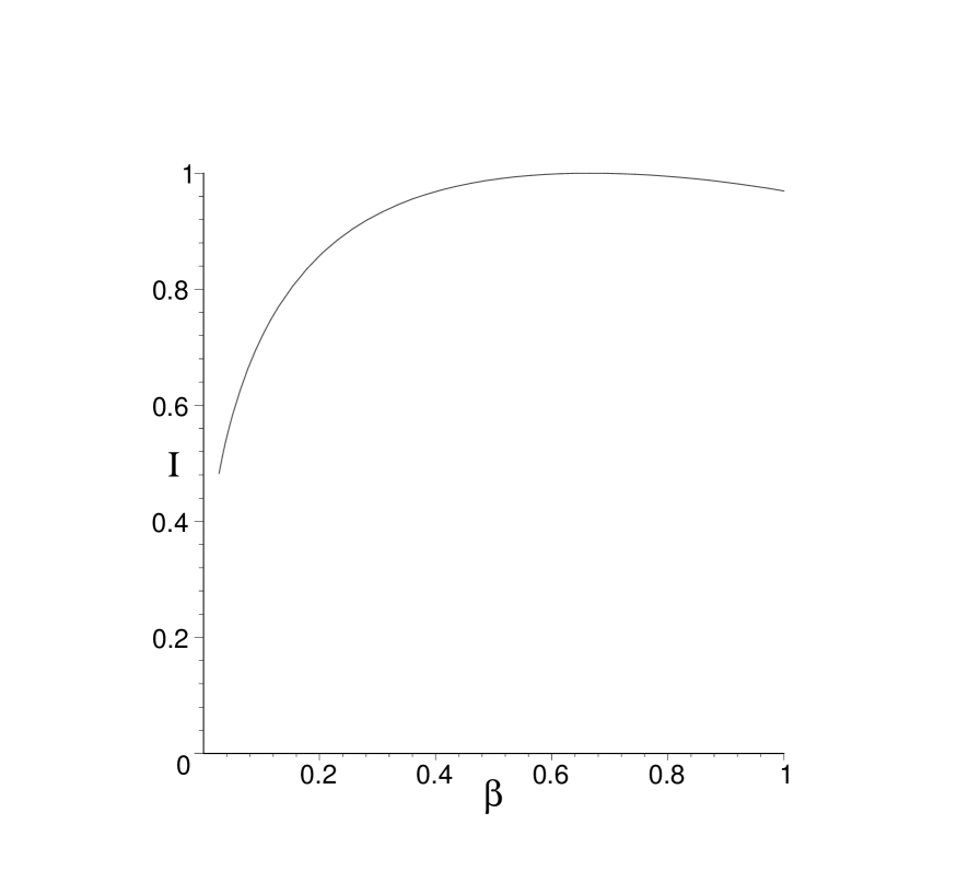
Figure 5: The ratio of information content about $\beta$ extracted through the angular moments method and the maximal likelihood method. The X-axis is the actual value of $\beta$.

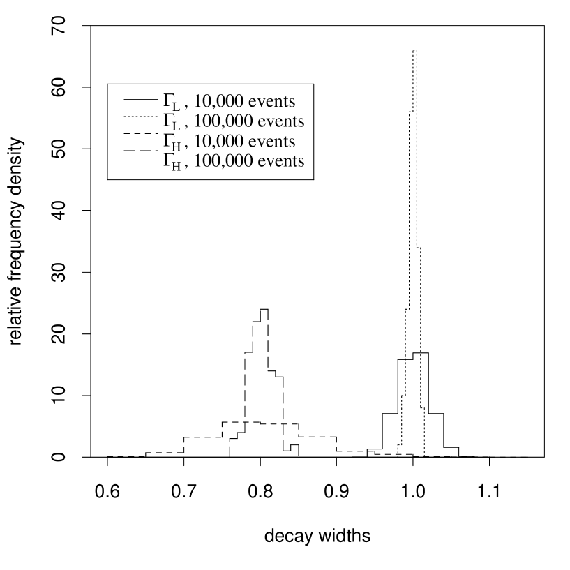
Figure 6: Determination of $\Gamma_{H}$ and $\Gamma_{L}$. The X-axis has been normalized to $\Gamma_{L}\mbox{\it(actual)}=1.0$.

Figure 7: Determination of $|A_{\|}/A_{0}|$. The solid line is for 10,000 events and the dashed line is for 100,000 events.

Figure 8: Determination of $|A_{\perp}/A_{0}|$.The solid line is for 10,000 events and the dashed line is for 100,000 events.

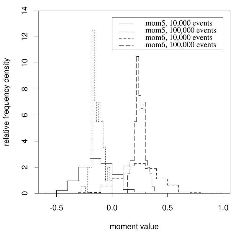
Figure 9: The moments of the “Im” terms in eq. 33. mom5 is the value of $-|A_{\|}||A_{\perp}|\cos(\delta_{1}+\kappa)\overline{\Gamma}/\sin\kappa$ and mom6 is the value of $-|A_{0}||A_{\perp}|\cos(\delta_{2}+\kappa)\overline{\Gamma}/\sin\kappa$.

References

- [1] G. Valencia, Phys. Rev. D39 (1989) 3339. G. Kramer and W.F. Palmer, Phys. Rev. D45 (1992) 193, Phys. Lett. B279 (1992) 181, Phys. Rev. D46 (1992) 2969 and 3197, G. Kramer, W.F. Palmer and H. Simma, Nucl. Phys. B428 (1994) 77; G. Kramer, T. Mannel and W.F. Palmer, Z. Phys. C55 (1992) 497 .
- [2] I. Dunietz, H. R. Quinn, A.. Snyder, W. Toki and H. J. Lipkin, Phys. Rev. D43 (1991) 2193.
- [3] A. S. Dighe, I. Dunietz and R. Fleischer, Preprints CERN-TH/98-85, IC/98/25, hep-ph/9804253. To be published in Eur. Phys. J. C.
- [4] J.S. Hagelin, Nucl. Phys. B193 (1981) 123; E. Franco, M. Lusignoli and A. Pugliese, ibid. B194 (1982) 403; L.L Chau, W.-Y. Keung and M. D. Tran, Phys. Rev. D27 (1983) 2145; L.L Chau, Phys. Rep. 95 (1983) 1; A.J. Buras, W. Slominski and H. Steger, Nucl. Phys. B245 (1984) 369; M.B. Voloshin, N.G. Uraltsev, V.A. Khoze and M.A. Shifman, Yad. Fiz. 46 (1987) 181 [Sov. J. Nucl. Phys. 46 (1987) 112]; A. Datta, E.A. Paschos and U. Türke, Phys. Lett. B196 (1987) 382; A. Datta, E.A.. Paschos and Y.L. Wu, Nucl. Phys. B311 (1988) 35; M. Lusignoli, Z. Phys. C41 (1989) 645; R. Aleksan, A. Le Yaouanc, L. Oliver, O. Pène and Y.-C. Raynal, Phys. Lett. B316 (1993) 567; I. Bigi, B. Blok, M. Shifman, N. Uraltsev and A. Vainshtein, in B Decays, ed. S. Stone, 2nd edition (World Scientific, Singapore, 1994), p. 132 and references therein; M. Beneke, G. Buchalla and I. Dunietz, Phys. Rev. D54 (1996) 4419.
- [5] R. Fleischer and I. Dunietz, Phys. Lett. B387 (1996) 361. R. Fleischer and I. Dunietz, Phys. Rev. D55 (1997) 259.
- [6] J.L. Rosner, Phys. Rev. D42 (1990) 3732.
- [7] A. S. Dighe, I. Dunietz, H. J. Lipkin and J. L. Rosner, Phys. Lett. B369 (1996) 144.
- [8] R. Aleksan, B. Kayser and D. London, Phys. Rev. Lett. 73 (1994) 18.
- [9] CDF Collaboration, F. Abe et al., Phys. Rev. Lett. 75 (1995) 3068.
- [10] CLEO Collaboration, CLEO Conf 96-24, ICHEP96 PA05-074.
- [11] D. R. Cox and D. V. Hinkley, Theoretical Statistics, Chapman and Hall, London (1974).
- [12] R. A. Thisted, Elements of Statistical Computing, Chapman and Hall, New York (1988).
- [13] The CDF II Detector Technical Design Report, CDF Collaboration, D. Amidei, ed. November 1996, FERMILAB-Pub-96/390-E
- [14] M. Beneke et. al., hep-ph/9808385.
- [15] M. Bauer, B. Stech and M. Wirbel, Z. Phys. C29 (1985) 637 and Z. Phys. C34 (1987) 103; J. M. Soares, Phys. Rev. D53 (1996) 241; H. Y. Cheng, Z. Phys. C69 (1996) 647.
- [16] A. S. Dighe, I. Dunietz and R. Fleischer, Phys. Lett. B433 (1998) 147.
- [17] P. Galumian, in preparation.
- [18] CLEO Collaboration, CLEO Conf 98-23, ICHEP98 852.