hep-ph/9810374

SHEP-98/13

Naturalness Implications of LEP Results

G. L. Kane¹ and S. F. King²

¹Randall Physics Laboratory, University of Michigan, Ann Arbor, MI 48109-1120
²Department of Physics and Astronomy, University of Southampton, Southampton, SO17 1BJ, U.K.

Abstract

We analyse the fine-tuning constraints arising from absence of superpartners at LEP, without strong universality assumptions. We show that such constraints do not imply that charginos or neutralinos should have been seen at LEP, contrary to the usual arguments. They do however imply relatively light gluinos $\left(m_{\tilde{g}}\lower 3.01385pt\hbox{$\;\stackrel{{\scriptstyle\textstyle<}}{{\sim}}\;$}350\rm{GeV}\right)$ and/or a relation between the soft-breaking $SU(3)$ gaugino mass and Higgs soft mass $m_{H_{U}}$. The LEP limit on the Higgs mass is significant, especially at low $\tan\beta$, and we investigate to what extent this provides evidence for both a lighter gluino and correlations between soft masses.

1 Introduction

There are several circumstantial pieces of evidence for supersymmetry (SUSY) not least of which are the measured magnitudes of the gauge coupling strengths at low energy which hint at a high energy unification for a light SUSY spectrum. This fits in well with a prime motivation for SUSY which is to protect the Higgs mass parameter from large radiative corrections, which again requires a light SUSY spectrum. Taken together these self-reinforcing pieces of circumstantial evidence provide rather convincing phenomenological support for what would in any case be an elegant extension of the standard model. However although the unification and fine-tuning arguments look quite convincing there are two areas of concern coming from recent LEP measurements. Our philosophy is that such areas of concern should be regarded as opportunities for new insights.

One such opportunity is the discrepancy between the world average experimental measurement of the strong coupling $\alpha_{3}(M_{Z})=0.119(4)$ and the value predicted from SUSY GUTs $\alpha_{3}(M_{Z})=0.13(1)$, an effect we think is significant even though the theoretical uncertainty is hard to quantify[1]. This difference may be telling us about aspects of the spectrum or of Planck scale physics. A second opportunity is due to the recent LEP limits on the mass of SUSY and Higgs particles and the implications this has for fine-tuning. In particular the absence of both charginos and Higgs at the highest energy LEP runs has been argued to significantly increase the fine-tuning “price” relative to what it was previously [2]. Earlier analyses which developed these fine-tuning arguments had raised expectations that SUSY particles should be found at LEP [3].

Here we take a constructive point of view that these mild quantitative difficulties referred to above are in fact useful pointers which are telling us something important about the SUSY spectrum. A common assumption, motivated by minimal supergravity (SUGRA), is that at high energies the SUSY spectrum is described by a universal soft scalar mass, $m_{0}$, and universal gaugino mass, $M_{1/2}$, which together with the universal trilinear parameter $A_{0}$ and the bilinear parameter $B_{0}$ and Higgs superpotential mass parameter $\mu_{0}$ form the five high energy input parameters of the constrained minimal supersymmetric standard model (CMSSM) [4]. Many of the unification and fine-tuning analyses presented in the literature are based completely or partially on the CMSSM, and of those analyses that do relax universality nearly all do so in the scalar sector while maintaining gaugino mass universality. From these assumptions, and the absence of superpartners at LEP, it is concluded by some authors that we should be nervous about the validity of the general SUSY framework. An exception is the unification analysis of Roszkowski and Shifman [5] which showed that by relaxing the assumption of gaugino mass unification, and allowing the gluino mass to be smaller than the wino mass at the GUT scale, $M_{3}(0)<M_{2}(0)$, the effect of low energy thresholds due to a lighter gluino and heavier wino is to push down the SUSY prediction of $\alpha_{3}(M_{Z})$ towards the experimental value. We will see below that the natural solution of the fine-tuning problem also reduces $\alpha_{3}(M_{Z})$, perhaps increasing our confidence in the relevence of our results.

Another exception is the fine-tuning analysis of Wright [6] which we were unaware of in a previous version of this paper. Wright also relaxes universality of the gaugino masses, and sets fine-tuning limits on the masses of superpartners. He concludes that the most problematic constraint arises from the gluino mass which is bounded to be less that 260 GeV corresponding to a fine-tuning limit of 10%. He also sets a fine-tuning limit on the $\mu$ parameter of 140 GeV. In hindsight the present paper serves to reaffirm Wright’s conclusions by including some details left out of the calculation of Wright (such as the running of the top quark Yukawa coupling) and also gives a qualitative analytic understanding of why the gluino mass plays such an important role in fine-tuning. We shall also address the role of the Higgs mass in fine-tuning, which was not covered by Wright. In addition we shall propose a genuinely new idea (as far as we are aware) which we call the supernatural solution to the fine-tuning opportunity.

In this paper, then, we investigate fine-tuning without the gaugino mass universality assumption . We focus on this because the usual results most strongly constrain charginos and neutralinos. We explore two ways to obtain small fine-tuning:

1. We show that having a gluino mass smaller than its universality value reduces the fine-tuning dramatically;

2. We suggest new theoretical correlations or simply relations between input parameters in order to reduce fine-tuning, such as a correlation or relation between $m_{H_{U}}$, the soft-breaking scalar mass that triggers the Higgs mechanism, and $M_{3}$, the $SU(3)$ gaugino mass that is proportional to the gluino mass, or between $\mu$ and the gluino mass (if $\mu$ is large).

We emphasise the distinction between a correlation and a relation between two input parameters. By a correlation we mean an exact theoretical relation such that the two parameters should no longer be regarded as independent, but instead should be regarded as a single input parameter. A relation on the other hand is simply a statement of the relative magnitude of one parameter relative to another. Clearly correlations have the potential to completely or partially alleviate fine-tuning if their correlation involves a partial cancellation of two large numbers to obtain a numerically small physical quantity, although the origin of such a desirable correlation may remain obscure. By contrast simple relations between parameters may lead to modest reductions in fine-tuning by simply moving to a different part of non-universal parameter space which is more favourable from the point of reducing the total (or global) amount of fine-tuning. We shall discuss correlations in the text and explore relations numerically.

Which of 1 or 2 holds, or whether both do, is fully testable experimentally. For example the first implies a physical $\tilde{g}$ mass less than about 350 GeV, possibly even around 250 GeV. For $\tan\beta\sim 1$ correlations are the only option, because the absence of a Higgs boson at LEP does not allow the gluino mass to be light enough to significantly reduce the fine-tuning (see below).

We emphasise that in the first case above we do not envisage a very light gluino such that it becomes the lightest supersymmetric particle (LSP) [7], but merely that it is somewhat lighter than the universal gaugino mass prediction, by an amount which we shall quantify in due course but which typically may be around 1/2 of its universal value. Also even though we abandon minimal SUGRA we shall stay within the general framework of the SUGRA mechanism of SUSY breaking for the present discussion, though many of our conclusions will apply also to gauge mediated SUSY breaking scenarios. We should also point out that the abandonment of universality fits in well with current ideas of string and M-theory in whose framework the minimal SUGRA model, which provided the theoretical impetus for the CMSSM, plays no special role. On the other hand the absence of flavour-changing neutral currents (FCNC’s) seems to imply that there must be a high degree of universality at least in flavour space. These arguments lead one to expect that the high energy soft SUSY breaking parameters could well contain as much non-universality as can be tolerated consistent with the absence of FCNC’s.

Following the above philosophy leads to the recently proposed so called minimal reasonable model (MRM) [8]. From the point of view of our solution to the fine-tuning problem the phases [8, 9] play no special role though they will certainly have quantitative effects if they are included, but we set them to zero for our qualitative study. We shall restrict ourselves to low and intermediate $\tan\beta$ for this analysis. With these additional assumptions the MRM depends only on the top quark Yukawa coupling $h_{t}(0)$ plus the following 13 real parameters $a$ at the unification scale $M_{U}$ where:

$$a\in\{m_{Q}^{2}(0),m_{U}^{2}(0),m_{D}^{2}(0),m_{L}^{2}(0),m_{E}^{2}(0),m_{H_{D}}^{2}(0),m_{H_{U}}^{2}(0),$$

$$M_{1}(0),M_{2}(0),M_{3}(0),A_{t}(0),B(0),\mu(0)\}$$ (1)

The notation is such that $t=\ln(M_{U}^{2}/Q^{2})$ where $Q$ is the $\bar{MS}$ energy scale, so that $t=0$ corresponds to $Q=M_{U}$. We do not have to choose between GUT and string unification. The version of MRM we use here includes an independent soft mass parameter for every chiral multiplet of the MSSM $Q^{i},U^{i},D^{i},L^{i},E^{i},H_{D},H_{U}$ in a common notation corresponding to quark doublets, up-type quark singlets, down-type quark singlets, lepton doublets, charged lepton singlets, Higgs doublet coupling to down-type quarks and charged leptons, Higgs doublet coupling to up-type quarks, respectively. At high energies the soft mass matrices in family space are assumed to be diagonal and family-independent (given by the 5 squark and slepton mass parameters in Eq.1 multiplying unit matrices) as motivated by the phenomenological requirement of acceptable FCNC’s. We are also implicitly assuming that the only soft trilinear parameter of importance is the one corresponding to the top Yukawa coupling, which again seems reasonable. We should also point out that the above parameter set in Eq.1 may be more than just an arbitrary choice. For example if the gaugino masses are large compared to the scalar masses at the string scale then the parameter set in Eq.1 (with additional relations between the soft masses) may be reproduced at a slightly lower scale as an infra-red fixed point in a class of theories [10]

One loop semi-analytic solutions to the renormalisation group equations corresponding to the above parameter set in Eq.1 have been presented in ref.[11] whose sign conventions for $A_{t},\mu,B$ we adopt. The solutions represent an extension of those in ref.[12]. The existence of analytic solutions in which the low energy diagonal masses

$$\{m_{Qi}^{2}(t),m_{Ui}^{2}(t),m_{Di}^{2}(t),m_{Li}^{2}(t),m_{Ei}^{2}(t),m_{H_{D}}^{2}(t),m_{H_{U}}^{2}(t),$$

$$M_{1}(t),M_{2}(t),M_{3}(t),A_{t}(t),B(t),\mu(t)\}$$ (2)

may be expressed in terms of the high energy parameters in Eq.1 is important because it enables fine-tuning (and the conditions for its absence) to be understood at a qualitative level.

2 Analysis

Let us begin our discussion of fine-tuning by recalling a few basic features of electroweak symmetry breaking in the MSSM, at the RG improved tree-level. The potential is:

$$V_{0}=m_{1}^{2}v_{1}^{2}+m_{2}^{2}v_{2}^{2}-2m_{3}^{2}v_{1}v_{2}+\frac{1}{8}(g^{\prime 2}+g_{2}^{2})(v_{1}^{2}-v_{2}^{2})^{2}$$ (3)

where $v_{1},v_{2}$ are the (assumed) neutral Higgs vacuum expectation values (VEVs), $g_{2},g^{\prime}$ are the $SU(2)_{L}\times U(1)_{Y}$ gauge couplings and the mass parameters $m_{1}^{2},m_{2}^{2},m_{3}^{2}$ are evaluated at low energy and are given by

$$m_{1}^{2}(t)=m_{H_{D}}^{2}(t)+\mu^{2}(t),\ \ m_{2}^{2}(t)=m_{H_{U}}^{2}(t)+\mu^{2}(t),\ \ m_{3}^{2}(t)=B(t)\mu(t)$$ (4)

The conditions for successful electroweak symmetry breaking are

$$m_{1}^{2}(t)m_{2}^{2}(t)-m_{3}^{4}(t)<0$$ (5)

$$m_{1}^{2}(t)+m_{2}^{2}(t)-2m_{3}^{2}(t)>0$$ (6)

where the first condition makes the symmetric case unstable, and the second condition ensures that the potential is bounded. These conditions are achieved in practice by virtue of the large top Yukawa coupling which drives $m_{2}^{2}(t)$ small and often negative. Assuming these conditions are met the minimisation conditions are expressable as:

$$\frac{M_{Z}^{2}}{2} = -\mu^{2}(t)+\left(\frac{m_{H_{D}}^{2}(t)-m_{H_{U}}^{2}(t)\tan^{2}\beta}{\tan^{2}\beta-1}\right)$$ (7)

$$\sin 2\beta = \frac{2m_{3}^{2}(t)}{m_{1}^{2}(t)+m_{2}^{2}(t)}$$ (8)

where

$$\tan\beta=v_{2}/v_{1},\ \ M_{Z}^{2}=\frac{1}{2}(g^{\prime 2}+g_{2}^{2})(v_{1}^{2}+v_{2}^{2})$$ (9)

The $U(1)_{Y}$ coupling normalised appropriately for unification is given by $g_{1}^{2}=(5/3)g^{\prime 2}$.

The principle of the electroweak symmetry breaking mechanism is that the high energy parameters in Eq.1 are fixed (presumably by some SUSY breaking mechanism in string theory). Then they run down to low energies and induce electroweak symmetry breaking along the above lines, with the Z mass and $\tan\beta$ predicted from a given set of input parameters.

The basic question of fine-tuning is one of the sensitivity of the electroweak scale, in this case expressed as the Z mass squared, to small variations in the input parameters which are perturbed around a particular physical solution corresponding to an acceptable Z mass. At a very basic level one may see the fine-tuning explicitly by expanding the formula for the Z mass squared Eq.7 in terms of the low energy masses in Eq.2 which in turn are expressed as a function of high energy input parameters in Eq.1 via the analytic solutions. For example for $\tan\beta=2.5$ we find

$$\frac{M_{Z}^{2}}{2}= \mbox{}-.87\,\mu^{2}(0)+3.6\,{M_{3}^{2}(0)}-.12\,{M_{2}^{2}(0)}+.007\,{M_{1}^{2}(0)}$$ (10)

$$\mbox{}-.71\,{m_{H_{U}}^{2}(0)}+.19\,{m_{H_{D}}^{2}(0)}+.48\,({m_{Q}^{2}(0)}+\,{m_{U}^{2}(0)})$$

$$\mbox{}-.34\,{A_{t}(0)}\,{M_{3}(0)}-.07\,{A_{t}(0)}\,{M_{2}(0)}-.01\,{A_{t}(0)}\,{M_{1}(0)}+.09\,{A_{t}^{2}(0)}$$

$$\mbox{}+.25\,{M_{2}(0)}\,{M_{3}(0)}+.03\,{M_{1}(0)}\,{M_{3}(0)}+.007\,{M_{1}(0)}\,{M_{2}(0)}$$

This is an important equation to examine. First, notice that the coefficients of terms involving $M_{1}(0)$ and $M_{2}(0)$, the soft mass parameters that determine the chargino and neutralino masses, are very small compared to those involving the high energy gluino mass $M_{3}(0)$. For $M_{3}(0)\gg M_{Z}$ it is necessary to tune $\mu^{2}(0)$ for a given $\tan\beta$ (which in turn is fixed by adjusting $B$) so that the large terms are cancelled and the correct Z mass is achieved. This is the fine-tuning problem. The solution to the fine-tuning problem is clearly to reduce $M_{3}(0)$ as much as possible since it has by far the largest coefficient. By contrast $M_{1}(0)$ and $M_{2}(0)$ may be increased almost arbitrarily without affecting fine-tuning. For $\tan\beta=1.5,2.5,10$ the coefficient of the $M_{3}^{2}(0)$ term is $6.1,3.6,2.8$ which shows that the fine-tuning problem is worse for low $\tan\beta$. Thus we conclude that the fine-tuning analysis mainly limits the gluino mass and only constrains the chargino and neutralino masses very weakly.

One can see from Eq.10 that there is a second way to overcome the apparent fine-tuning problem, namely to invoke theoretical correlations between $M_{3}(0)$ and any parameter which enters with a negative sign, such as $\mu(0),m_{H_{U}}^{2}(0),A_{t}(0),M_{2}(0)$. The idea of a correlation between $\mu(0)$ and the universal gaugino mass $M_{1/2}$ is well known (see for example Chankowski et al [2]). From our point of view this would become a correlation between $\mu(0)$ and $M_{3}(0)$, and it could only be relevant for large $\mu(0)$. We can identify other perhaps more plausible correlations. For example, suppose that the fundamental theory after supersymmetry breaking led to $m_{H_{U}}(0)\approx 2M_{3}(0)$. Then the combination of the $m^{2}_{H_{U}}(0)$ and $M_{3}^{2}(0)$ terms has a coefficient less than or of order unity, as do all other terms, and there is no fine-tuning problem. Presumably other terms would enter into the true relation, but the essential feature is that between $m_{H_{U}}(0)$ and $M_{3}(0)$. We regard such correlations between soft masses to be more likely than a correlation involving $\mu$ which is not a soft mass.

If relatively light gluinos are found experimentally (say 200 $\lower 3.01385pt\hbox{$\;\stackrel{{\scriptstyle\textstyle<}}{{\sim}}\;$}m_{\tilde{g}}\lower 3.01385pt\hbox{$\;\stackrel{{\scriptstyle\textstyle<}}{{\sim}}\;$}350\>{\rm GeV})$ then apparently the fine-tuning problem is solved by small $M_{3}(0)$, while if the gluino mass is larger it implies correlations such as between $M_{3}(0)$ and $m_{H_{U}}(0)$. Such a relation would be an important clue to the form of SUSY breaking of string theory. By such reasoning we could learn about the form of unification or Planck scale physics from collider data, even before superpartners are found!

The above qualitative discussion takes no account of the implicit sensitivity of the Z mass coming from changes in $\tan\beta$ as a result of small variations in the high energy inputs. This is addressed by the master formula of Dimopoulos and Giudice [3] which yields a fine-tuning parameter which corresponds to the fractional change in the Z mass squared per unit fractional change in the input parameter,

$$\Delta_{a}=abs\left(\frac{a}{M_{Z}^{2}}\frac{\partial M_{Z}^{2}}{\partial a}\right)$$ (11)

for each input parameter $a$ in Eq.1. Following the above discussion it is sufficient for our purposes to calculate three parameters $\Delta_{\mu(0)}$, $\Delta_{M_{3}(0)}$ and $\Delta_{m_{H_{U}}^{2}(0)}$. As with the Z mass we may expand these fine-tuning parameters in terms of the high energy input parameters, and so investigate the source of the fine-tuning. For $\tan\beta=2.5$ we find

$$\Delta_{\mu(0)} \approx 5.1\tilde{\mu}^{2}(0)+2.7\,{\tilde{M}_{3}^{2}(0)}-0.6\,{\tilde{M}_{2}^{2}(0)}-.03\,{\tilde{M}_{1}^{2}(0)}$$ (12)

$$- .54\,{\tilde{m}_{H_{U}}^{2}(0)}-.91\,{\tilde{m}_{H_{D}}^{2}(0)}+.36\,({\tilde{m}_{Q}^{2}(0)}+\,{\tilde{m}_{U}^{2}(0)})$$

$$- .26\,{\tilde{A}_{t}(0)}\,{\tilde{M}_{3}(0)}-.06\,{\tilde{A}_{t}(0)}\,{\tilde{M}_{2}(0)}-.009\,{\tilde{A}_{t}(0)}\,{\tilde{M}_{1}(0)}+.07\,{\tilde{A}_{t}(0)}^{2}$$

$$+ .19\,{\tilde{M}_{2}(0)}\,{\tilde{M}_{3}(0)}+.03\,{\tilde{M}_{1}(0)}\,{\tilde{M}_{3}(0)}+.005\,{\tilde{M}_{1}(0)}\,{\tilde{M}_{2}(0)}$$

where the tilde denotes that the parameter is scaled by $M_{Z}$. It is possible to eliminate $\mu^{2}(0)$ using Eq.10, which would lead to a dominant term $23.7\,{\tilde{M}_{3}^{2}(0)}$. For $\tan\beta=1.5,2.5,10$ the coefficient of the $\tilde{M}_{3}^{2}(0)$ term is $115,24,12$.

As with Eq.10, Eq.12 shows that there is greatly reduced sensitivity to $M^{2}_{1}(0)$ or $M^{2}_{2}(0)$ compared to $M_{3}^{2}(0)$. The fine-tuning from Eq.12 is in fact much worse than anticipated from Eq.10 due to the implicit $\tan\beta$ sensitivity. It is clear that once either $\tilde{M}_{3}(0)$ or $\tilde{\mu}^{2}(0)$ become larger than unity then the amount of fine-tuning grows quadratically. The effect is ameliorated to some extent by the negative contributions coming from ${\tilde{m}_{H_{U}}^{2}(0)}$, ${\tilde{M}_{2}^{2}(0)}$ and the terms proportional to ${\tilde{A}_{t}(0)}$. But such terms cannot be made arbitrarily large since then the fine-tuning parameters associated with them will become important, unless we postulate some theoretical correlation between them.

Having shown that the gluino mass parameter is largely responsible for fine-tuning, let us briefly take stock of how this comes about. Naively, one might think that the physics of electroweak symmetry breaking (EWSB) is purely related to physics in the electroweak sector, and the existence of a large top Yukawa coupling. As it is normally portrayed, $m^{2}_{H_{U}}$ runs and becomes negative if one simply includes a large top Yukawa in its renormalisation group equation (RGE). However QCD plays an important role in EWSB by ensuring that the squark masses, and especially $m^{2}_{U_{3}}$ is not driven more negative, leading to charge and colour breaking minima being preferred. The Higgs mass parameter $m^{2}_{H_{U}}$ feels QCD effects via the top Yukawa coupling (which itself depends on QCD effects for its magnitude) and the gluino mass which thereby enters turns out to dominate due to the relatively fast variation of the QCD coupling as compared to the electroweak couplings:

$$\left(\frac{\alpha_{1}(t)}{\alpha_{1}(0)}\right)\approx\frac{5}{12},\ \ \left(\frac{\alpha_{2}(t)}{\alpha_{2}(0)}\right)\approx\frac{10}{12},\ \ \left(\frac{\alpha_{3}(t)}{\alpha_{3}(0)}\right)\approx\frac{32}{12},$$ (13)

where $t=\ln(M_{U}^{2}/M_{Z}^{2})\approx 66$.

3 Higgs Mass Constraints

Having argued that the absence of charginos and neutralinos at LEP is only weakly related to fine-tuning issues, now let us turn to the question of the lightest CP even Higgs boson (henceforth simply called the Higgs). At tree-level the Higgs mass is given by $m_{h}^{0}\approx M_{Z}|\cos 2\beta|$ with $m_{h}^{0}=35,66,89$ GeV for $\tan\beta=1.5,2.5,10$, to be compared to the current LEP limit on the standard model Higgs mass roughly given by about 90 GeV but being reduced to 75 GeV or so (when SUSY effects and phases are fully included).

It is well known that radiative corrections play an important role for the Higgs [13]. A simplified expression for radiatively corrected Higgs mass includes the terms

$$m_{h}^{2}\approx M_{Z}^{2}\cos^{2}2\beta+(34\ GeV)^{2}\ln\left(\frac{m_{\tilde{t}_{1}}^{2}m_{\tilde{t}_{2}}^{2}}{m_{t}^{4}}\right)+\ldots$$ (14)

where the ellipsis represents more complicated terms. It is clear that the radiative corrections depend logarithmically on the determinant of the matrix of stop masses, at least for the second term, and in a more complicated way for the remaining terms. We can expand the determinant of the stop matrix, which involves the off-diagonal element $m_{t}(A_{t}-\mu\cot\beta)$, as a function of the high energy input parameters, and for $\tan\beta=2.5$ we find a lengthy expression whose leading terms are,

$${m_{\tilde{t}_{1}}^{2}m_{\tilde{t}_{2}}^{2}} \approx (170\ GeV)^{4}+26\,{M_{3}^{4}(0)}+1.5\,{A_{t}(0)}\,{M_{3}^{3}(0)}$$ (15)

$$\mbox{}+\left(2.5\,{m_{Q}^{2}(0)}+3.5\,{m_{U}^{2}(0)}-2.1\,{m_{H_{U}}^{2}(0)}\right)\,{M_{3}^{2}(0)}$$

$$\mbox{}+(134\ GeV)^{2}\,{m_{Q}^{2}(0)}+(130\ GeV)^{2}\,{m_{U}^{2}(0)}-(108\ GeV)^{2}\,{m_{H_{U}}^{2}(0)}$$

$$\mbox{}+(430\ GeV)^{2}\,{M_{3}^{2}(0)}-(180\ GeV)^{2}M_{2}(0)M_{3}(0)$$

$$\mbox{}+(180\ GeV)^{2}\,{A_{t}(0)}\,{M_{3}(0)}-(59\ GeV)^{2}\,{A_{t}^{2}(0)}-(65\ GeV)^{2}\,\mu^{2}(0)$$

$$\mbox{}+(67\ GeV)^{2}\,{A_{t}(0)}\,\mu(0)-(210\ GeV)^{2}\,{M_{3}(0)}\,\mu(0)$$

Taken together Eqs.14 and 15 show that any shortfall in the tree-level contribution to the Higgs mass must be compensated by exponential increases in stop masses, which in turn involves exponential increases in $M_{3}(0)$, and hence from Eqs.10, 12 exponential increases in fine-tuning. The exponential sensitivity of fine-tuning to the Higgs mass (for a fixed $\tan\beta$) was observed previously numerically [2].

It is clear that low values of $\tan\beta$ are associated with large fine-tuning for two quite distinct reasons. The first reason we saw from Eqs.10, 12, where the $M_{3}(0)$ coefficient grows alarmingly as $\tan\beta$ approaches unity. The second reason is that we have just seen that $M_{3}(0)$ itself (and to a lesser extent $A_{t}(0),m_{Q3}(0),m_{U3}(0)$) must grow exponentially if the Higgs mass is to remain acceptable as $\tan\beta$ is reduced. Any reduction in $M_{3}(0)$, such as that proposed in the previous section, to alleviate the fine-tuning problem, will clearly lead to a reduction in stop masses, and hence the contribution from radiative corrections to the Higgs mass. Of course such a reduction in the Higgs mass is easily compensated by increasing $\tan\beta$ slightly which will readily yield a compensating tree-level contribution. Thus, provided $\tan\beta$ is not too low, fine-tuning as a result of the non-observation of Higgs at LEP may also be avoided. If however one insists upon having very low values of $\tan\beta$ close to unity, then correlations between $M_{3}(0)$ and parameters such as $m_{H_{U}}(0)$ may allow large values of these parameters, and hence acceptable Higgs masses, without fine-tuning. However even in this case there will be a lower limit on $\tan\beta$ once radiative correction parameters such as $\Delta\rho$ are taken into account [14].

4 Numerical Estimates

In order to see the effect of lowering $M_{3}(0)$, and of correlations, as a function of $\tan\beta$, it is necessary to make some quantitative estimates of the fine-tuning parameters for different input parameters and to examine the corresponding physical spectra.

Figure 1 shows how the Higgs mass $m_{h}$ and fine-tuning parameter $\Delta_{\mu(0)}$ vary as a function of $\tan\beta$ for $M_{3}(0)=200,150,100$ GeV with the other soft masses held at universal values $m_{0}=100$ GeV, $M_{1,2}(0)=200$ GeV in each case. The Higgs mass has the full one-loop radiative corrections included. As $M_{3}(0)$ is reduced the fine-tuning parameter $\Delta_{\mu(0)}$ drops like a stone, as does $\Delta_{M_{3}(0)}$ which will be discussed separately. From the point of view of fine-tuning the $M_{3}(0)=100$ GeV case is clearly preferred with $\tan\beta\approx 2.5-10$ giving $\Delta_{\mu(0)}\approx 20-10$ and $m_{h}\approx 90-107$ GeV. The lower value of $M_{3}(0)$ leads to lower squark and gluino masses, and lighter stops which cause the Higgs mass to be reduced. Another direct effect of the reduction of fine-tuning is the decrease in the value of $\mu(M_{Z})$ which causes chargino and neutralino masses to fall and become more Higgsino-like, especially for larger $\tan\beta$. The lighter chargino (of mass $m_{\tilde{\chi}_{1}^{\pm}}\approx 100-88$ GeV for $\tan\beta\approx 2.5-10$) and neutralino may be made heavier by increasing $M_{1,2}$, without any additional fine-tuning expense. In the limit $\mu(M_{Z})\ll M_{2}(M_{Z})$, where the lighter chargino mass is essentially just $\mu(M_{Z})$, LEP limits on the lighter chargino translate directly into limits on $\mu(M_{Z})$. Since the fine-tuning parameter $\Delta_{\mu(0)}$ in Eq.12 has a strong $\mu$ dependence the LEP limits on chargino masses will always have some effect on fine-tuning, but in practice the lighter chargino mass may be increased by increasing $M_{2}(0)$ without incurring any additional fine-tuning expense. Finally we note that $\alpha_{3}(M_{Z})$ decreases by about 5% over the range $M_{3}(0)=200-100$ GeV, due to the decreasing gluino and squark mass thresholds. Including the gluino mass one-loop radiative corrections [15] we find $m_{\tilde{g}}\approx 284$ GeV independently of $\tan\beta$ for $M_{3}(0)=100$ GeV.

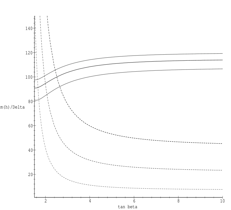
Figure 1: The Higgs mass $m_{h}$ (in GeV) (solid) and fine-tuning parameter $\Delta_{\mu(0)}$ (dashes) as a function of $\tan\beta$. The upper to lower curves correspond to $M_{3}(0)=200,150,100$ GeV. Apart from the gluino mass we use universal parameters $m_{0}=100$ GeV, $M_{1,2}(0)=200$ GeV in each case. Note the large decrease in the measure of fine-tuning as $M_{3}(0)$ decreases.

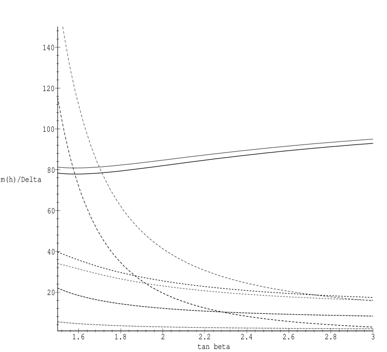
Figure 2: The Higgs mass $m_{h}$ (in GeV) (solid) and fine-tuning parameters (dashes) $\Delta_{\mu(0)}$, $\Delta_{M_{3}(0)}$, $\Delta_{m_{H_{U}}^{2}(0)}$ as a function of $\tan\beta$, for two parameter sets. The first parameter set corresponds to $M_{3}(0)=m_{0}=100$ GeV, $M_{1,2}(0)=200$ GeV and the second parameter set has all parameters unchanged apart from a larger second Higgs mass parameter $m_{H_{U}}(0)=200$ GeV. The $m_{h}$, $\Delta_{\mu(0)}$ curves are obviously identified by comparison to Figure 1. In fact the uppermost values of $m_{h}$, $\Delta_{\mu(0)}$ in this Figure correspond exactly to the lowermost values in Figure 1 which also uses the first parameter set here; note the change of scale for $\tan\beta$. The four remaining dashed lines correspond to $\Delta_{M_{3}(0)}$ (higher pair) and $\Delta_{m_{H_{U}}^{2}(0)}$ (lower pair), where now $m_{H_{U}}(0)=200$ GeV gives the upper curve of each pair. Observe here that by increasing $m_{H_{U}}(0)$ relative to $M_{3}(0)$ there is an additional decrease in the fine-tuning parameter $\Delta_{\mu(0)}$ which is particularly relevant for small $\tan\beta$ where it may be needed.

It is clear from Figure 1 that the idea of reducing $M_{3}(0)$, whilst leading to substantial reductions in fine-tuning for $\tan\beta\lower 3.01385pt\hbox{$\;\stackrel{{\scriptstyle\textstyle>}}{{\sim}}\;$}2.5$ is not by itself able to lead to a natural theory for lower values of $\tan\beta$. In order to reduce fine-tuning further in the low $\tan\beta$ region we would ideally like to reduce $M_{3}(0)$ significantly below 100 GeV, but we are effectively prevented from doing so because this would result in the Higgs mass becoming too light. The reduction in Higgs mass cannot be countered by increasing the soft masses $m_{Q}(0),m_{U}(0)$ which only leads to relatively modest increases in Higgs mass, which is dominated by $M_{3}(0)$ according to Eqs.14 and 15, and only results in additional fine-tuning in $\Delta_{\mu(0)}$ according to Eq.12. Therefore in order to reduce fine-tuning further we turn to the idea mentioned in section 2 which is to have a correlation or relation $m_{H_{U}}(0)\approx 2M_{3}(0)$. If it is a genuine correlation then the fine-tuning is automatically reduced by an amount which depends on how accurately the two quantities cancel. However if it is simply a relation then $m_{H_{U}}(0)$ cannot be increased abitrarily because it will have its own fine-tuning parameter which should not be too large. Therefore it becomes a quantitative question as to how much fine-tuning can genuinely be reduced in this case before the fine-tuning parameter $\Delta_{m_{H_{U}}^{2}(0)}$ becomes so large that additional correlations may be relevant. Figure 2 addresses this question.

In Figure 2 we plot the Higgs mass $m_{h}$ and fine-tuning parameters $\Delta_{\mu(0)}$, $\Delta_{M_{3}(0)}$, $\Delta_{m_{H_{U}}^{2}(0)}$ for two parameter sets, concentrating on the low $\tan\beta$ region. The first parameter set is already familiar from Figure 1 and corresponds to the smallest fine-tuning shown there ($M_{3}(0)=m_{0}=100$ GeV, $M_{1,2}(0)=200$ GeV). In Figure 2 this corresponds to the upper Higgs mass and $\Delta_{\mu(0)}$ curves and the lower $\Delta_{M_{3}(0)}$ and $\Delta_{m_{H_{U}}^{2}(0)}$ curves. For the first parameter set, it is clearly seen that $\Delta_{\mu(0)}$ used in Figure 1 is the dominant source of fine-tuning up to $\tan\beta=3$ beyond which $\Delta_{M_{3}(0)}$ becomes more important. For $\tan\beta\lower 3.01385pt\hbox{$\;\stackrel{{\scriptstyle\textstyle<}}{{\sim}}\;$}2.5$, $\Delta_{\mu(0)}$ grows sharply. By contrast $\Delta_{m_{H_{U}}^{2}(0)}$ is always very small and corresponds to the lowest line running along the bottom of the figure.

The second parameter set in Figure 2 only differs by having $m_{H_{U}}(0)=2M_{3}(0)=200$ GeV, motivated by the qualitative arguments presented in section 2. This results in only a 3 GeV decrease in the physical Higgs mass corresponding to the lower solid curve. However it also results in a large reduction in $\Delta_{\mu(0)}$ corresponding to the lower large-dashed curve, which permits smaller $\tan\beta$ to be reached for a given amount of fine-tuning. The difference between the $\Delta_{\mu(0)}$ curves in Figure 2 (the reduction in fine-tuning ) is about the same as between pairs of $\Delta_{\mu(0)}$ curves in Figure 1 where the reduction in Higgs mass is much greater. Furthermore $\Delta_{m_{H_{U}}^{2}(0)}$, although larger than before, is only about a half of $\Delta_{M_{3}(0)}$, which shows that at least for $m_{H_{U}}(0)=200$ GeV there is no additional price to pay there. We conclude that for small $\tan\beta$ there is a significant reduction in fine-tuning for the case $m_{H_{U}}(0)\approx 2M_{3}(0)$ as compared to $m_{H_{U}}(0)\approx M_{3}(0)$, with only a relatively small reduction in $m_{h}$. For larger $\tan\beta$ where fine-tuning is controlled by $\Delta_{M_{3}(0)}$, this mechanism does not reduce fine-tuning, but in that region fine-tuning is relatively small in any case. We note that if one attempts to increase $m_{H_{U}}(0)$ much further then $\Delta_{m_{H_{U}}^{2}(0)}$ will dominate the fine-tuning. Clearly then there is always a limit to how low $\tan\beta$ can become before fine-tuning grows uncontrollably, even using both low $M_{3}(0)$ and $m_{H_{U}}(0)\approx 2M_{3}(0)$ at the same time. If $\tan\beta$ is in fact very near unity, then a simple relation is insufficient, and we need to appeal to a genuine correlation between the input parameters.

Finally, on a phenomenological note, we remark that low $\tan\beta$ is often accompanied by a light stop squark. In this case, if the gluino is lighter than all the other squarks (achieved for example by $M_{3}(0)=100$ GeV, $m_{0}=200$ GeV) the dominant decay of the gluino will be $\tilde{g}\rightarrow\tilde{t}_{1}+t$ which may be observed at the Tevatron, and which may be the source of many tops there [17].

5 Conclusions

By analyzing EWSB without universality assumptions we are led to conclusions quite different from the usual ones. Our first observation is that the gaugino masses $M_{1}$ and $M_{2}$ are hardly constrained by the EWSB conditions, and also the $\mu$ parameter is not as severely constrained as $M_{3}$, so the masses of charginos and neutralinos can be larger without affecting fine-tuning. Therefore the absence of charginos at LEP does not imply large fine-tuning. Note that this conclusion is in agreement with that of Wright [6] who sets fine-tuning limits on charginos and neutralinos of about 160 GeV. The question of the Higgs at LEP is much more interesting and subtle. For $\tan\beta\lower 3.01385pt\hbox{$\;\stackrel{{\scriptstyle\textstyle>}}{{\sim}}\;$}2.5$ and $M_{3}(0)\approx 100$ GeV it is clear from Figure 1 that the present LEP limits on the Higgs mass involve relatively small fine-tuning, although more stringent future Higgs limits will require larger $\tan\beta$, or larger $M_{3}$ which would result in increased fine-tuning. Smaller values of $\tan\beta$ can be achieved without increasing fine-tuning by having $m_{H_{U}}(0)\approx 2M_{3}(0)$, in addition to a lighter gluino mass, as illustrated in Figure 2.

Of course fine-tuning is not a well defined concept so firm quantitative conclusions are difficult to draw. However regardless of one’s measure of fine-tuning the main qualitative constraint is on the $SU(3)$ gaugino mass $M_{3}$, and therefore on the gluino mass, which cannot get too large. We have identified two new ways to significantly reduce fine-tuning: $M_{\tilde{g}}\lower 3.01385pt\hbox{$\;\stackrel{{\scriptstyle\textstyle<}}{{\sim}}\;$}350$ GeV, and/or there is some correlation between $m_{H_{U}}$ and $M_{3}$, approximately that $m_{H_{U}}(0)\approx 2M_{3}(0)$, perhaps with additional contributions from squark soft masses or $A_{t}$ or $\mu$. A strict correlation might not be necessary since even a simple relation between these two input parameters, which are regarded as independent, may reduce fine-tuning as shown in Figure 2. Another possible correlation is between $\mu$ and $M_{3}$ if $\mu$ is large. It is very interesting that a lighter gluino pushes down the predicted $\alpha_{3}(M_{Z})$ towards the experimental value, as discussed in the introduction.

In this paper we have made no effort to fit or optimize fine-tuning parameters, because we do not believe any particular measure or value is much to be preferred. But we do believe that the general notion of a fine-tuning constraint is real and important, and we think it is telling us significant information about the soft-breaking masses. Most likely $M_{3}$ is smaller than its universality value relative to $M_{1}$ and $M_{2}$, and in addition perhaps $M_{3}$ and $m_{H_{U}}$ are related, particularly if $\tan\beta$ is small. Both ways we learn something about unification scale physics from collider data — either gaugino mass universality is violated (perhaps by as much as a factor of two), or there is a relation among soft-breaking parameters, or both. It will be possible to distinguish between these at the Fermilab upgraded collider.

Acknowledgements

SFK would like to thank Fermilab and University of Michigan Theory Groups for hospitality extended, and Marcela Carena for discussions. GLK appreciates discussions with Stefan Pokorski and Lisa Everett.

References

- [1] P. Langacker and N. Polonski, Phys. Rev. D 52 (1995) 3081.
- [2] P. Chankowski, J. Ellis and S. Pokorski, Phys. Lett. B 423 (1998) 327; R. Barbieri and A. Strummia, Phys. Lett. B 433 (1998) 63; P. Chankowski, J. Ellis, M. Olechowski and S. Pokorski, hep-ph/9808275; Kwok Lung Chan, Utpal Chattopadhyay, and Pran Nath, hep-ph/9710473.
- [3] J. Ellis, K. Enqvist, D. Nanopoulos and F. Zwirner, Nucl. Phys. B 276 (1986) 14; R. Barbieri and G.-F. Giudice, Nucl. Phys. B 306 (1988) 63; G. W. Anderson and D. J. Castano, Phys. Lett. B 347 (1995) 300; G. W. Anderson and D. J. Castano, Phys. Rev. D 52 (1995) 1693; G. W. Anderson and D. J. Castano, Phys. Rev. D 53 (1996) 2403; G. W. Anderson, D. J. Castano and A. Riotto, Phys. Rev. D 55 (1997) 2950; S. Dimopoulos and G.-F. Giudice, Phys. Lett. B 357 (1995) 573.
- [4] G. L. Kane, C.Kolda, L. Roszkowski and J. D. Wells, Phys. Rev. D 49 (1994) 6173.
- [5] L. Roszkowski and M. Shifman, Phys. Rev. D 53 (1996) 404.
- [6] D. Wright, hep-ph/9801449, UW/PT-97/27 (unpublished).
- [7] S. Raby and K. Tobe, hep-ph/9807281; S. Raby, Phys. Lett. B 422 (1998) 158; S. Raby, Phys. Rev. D 56 (1997) 2852; H. Baer, K. Cheung, J. F. Gunion, UCD-98-8, hep-ph/9806361.
- [8] M. Brhlik and G. L. Kane, hep-ph/9803391; M. Brhlik and G. L. Kane, in preparation.
- [9] T. Ibrahim, P. Nath, Phys. Lett. B 418 (1998) 98; T. Ibrahim, P. Nath, Phys. Rev. D 57 (1998) 478, Erratum-ibid. D 58 (1998) 019901; T. Ibrahim, P. Nath, hep-ph/9807501; T. Falk, A. Ferstl, K. A. Olive UMN-TH-1707-98, hep-ph/9806413; T. Falk, K. A. Olive UMN-TH-1705-98, hep-ph/9806236.
- [10] S. F. King and G. G. Ross, hep-ph/9803463 (Nucl.Phys.B in press).
- [11] M. Carena, P. Chankowski, M. Olechowski, S. Pokorski, C.E.M. Wagner, Nucl. Phys. B 491 (1997) 103.
- [12] L. E. Ibanez, C. Lopez and C. Munoz, Nucl. Phys. B 256 (1985) 218.
- [13] H. Haber and R. Hempfling, Phys. Rev. Lett. 66 (1991) 1815; Y. Okada, M. Yamaguchi and T. Yanagida, Prog. Theor. Phys. 85 (1991) 1; J. Ellis, G. Ridolfi and F. Zwirner, Phys. Lett. B 257 (1991) 83; J. Ellis, G. Ridolfi and F. Zwirner, Phys. Lett. B 262 (1991) 477.
- [14] M. Carena, P.H. Chankowski, S. Pokorski, C.E.M. Wagner, hep-ph/9805349; J. Casas, J. R. Espinosa and H. Haber, hep-ph/9801365.
- [15] S. P. Martin, M. T. Vaughn, Phys. Lett. B 318 (1993) 331; D. M. Pierce, J. A. Bagger, K. Matchev, Ren-jie Zhang Nucl. Phys. B 491 (1997) 3.
- [16] M. Carena, S. Mrenna and C. E. M. Wagner, hep-ph/9808312.
- [17] G. L. Kane and S. Mrenna, Phys. Rev. Lett. 77 (1996) 3502.