Abstract

Exclusive decays of $B$ and $D$ mesons are discussed with the focus on the theoretical problem how to calculate the relevant hadronic matrix elements of weak operators in the framework of QCD sum rules. The three lectures are devoted to
                           1. leptonic decays and decay constants
                           2. semileptonic decays and form factors
                           3. nonleptonic decays and nonfactorizable amplitudes.
I shall introduce some of the basic concepts, describe various calculational techniques, and illustrate the numerical results. The latter are compared with lattice and quark model predictions and, where possible, with experimental data. Applications include the determination of $V_{ub}$ from $B\rightarrow\pi\bar{l}\nu_{l}$ and $B\rightarrow\rho\bar{l}\nu_{l}$, and an estimate of the phenomenological coefficient $a_{2}$ for $B\rightarrow J/\psi K$.

1 Introduction

Inclusive and exclusive decays of heavy flavours play a complementary role in the determination of fundamental parameters of the electroweak standard model and in the development of a deeper understanding of QCD. While the theory of inclusive decays is well advanced, inclusive measurements are generally quite difficult. Conversely, exclusive decays into few-body final states are often easier to measure, but the theory of exclusive processes is more demanding and hence still underdeveloped. In view of the exciting experimental prospects at future bottom and charm factories, where many exclusive channels are expected to be measured accurately, it is pressing to make further progress on the theoretical side.

The difference in complexity of inclusive and exclusive observables is illuminated by the fact that the simple parton picture of charm and beauty decays illustrated in Tab. 1 provides surprisingly reasonable estimates for the lifetimes and inclusive branching ratios, whereas no such description exists for exclusive decays. The theory of both inclusive and exclusive processes is based on operator product expansion (OPE) which allows to separate the dynamics at short and long distances. At very large scale, $\mu=O(m_{W})$, charm and beauty decays are described by second order weak interaction involving $W$ exchange. Since the momentum transfer $p^{2}\ll m_{W}^{2}$, one effectively has four-fermion interactions described by a hamiltonian of the form

$$H_{W}=\frac{G_{F}}{\sqrt{2}}j^{\mu}j^{\prime}_{\mu}~{},$$ (1.1)

where $j_{\mu}$ and $j^{\prime}_{\mu}$ are $V-A$ quark or lepton currents. In the nonleptonic case, evolution of the hamiltonian to the physical scale of the order of the heavy quark mass, $\mu=O(m_{Q})$, leads to considerable modifications of (1.1) due to strong interactions. These effects can be taken into account by OPE and renormalization group methods. The result is an effective hamiltonian

$$H_{NL}=\frac{G_{F}}{\sqrt{2}}\sum_{i}c_{i}(\alpha_{s},\mu)O_{i}(\mu)$$ (1.2)

involving a sum of local operators $O_{i}$ with coefficients $c_{i}$ which can be calculated in perturbation theory as long as $\mu\gg\Lambda_{QCD}$ so that one is only dealing with interactions of quarks and gluons at short distances. The decay amplitudes are then given by

$$A(P\to X_{h})=\frac{G_{F}}{\sqrt{2}}\sum_{i}c_{i}(\alpha_{s},\mu)\langle X_{h}\mid O_{i}(\mu)\mid P\rangle$$ (1.3)

showing the main problem, that is the calculation of the matrix elements of the weak operators $O_{i}$ which incorporate the long-distance effects. For semileptonic decays one instead has to compute matrix elements of weak currents:

$$A(P\to l\bar{\nu}_{l}X_{h})=\frac{G_{F}}{\sqrt{2}}\langle X_{h}\mid j_{\mu}\mid P\rangle\langle l\bar{\nu_{l}}\mid j^{\prime}_{\mu}\mid 0\rangle~{}.$$ (1.4)

This simplifies the problem.

The usual way to proceed in inclusive decays is to assume duality of the sum over all possible hadronic states $X_{h}$ and the quark (and gluon) final states. The theory is further improved by including radiative corrections to the decay widths, quark mass effects, and initial bound state corrections [1]. In comparison, the calculation of the hadronic matrix elements in (1.3) and (1.4) for exclusive final states $X_{h}$ constitutes an ab initio nonperturbative problem. Tab. 2 illustrates typical exclusive decays considered in these lectures, and the corresponding matrix elements such as decay constants, form factors and nonleptonic two-body amplitudes. Here, the interplay between weak and strong interactions is even more intricate than in inclusive decays. Obviously, in order to disentangle the properties of weak interactions such as the charged current structure, flavour mixing and CP violation from exclusive processes, one must understand the impact of QCD beyond perturbation theory.

Current approaches include lattice calculations, QCD sum rules, heavy quark effective theory (HQET), chiral perturbation theory (CHPT), and phenomenological quark models. Each of these approaches has advantages and disadvantages. For example, quark models are easy to use and good for intuition. However, their relation to QCD is unclear. On the other hand, lattice calculations are rigorous from the point of view of QCD, but they suffer from lattice artifacts and uncertain extrapolations. Furthermore, effective theories are usually applicable only to a restricted class of problems, and sometimes require substantial corrections which cannot be calculated within the same framework. For example, HQET is very powerful in treating $b\rightarrow c$ transitions, but a priori less suitable for $b\to u$ transitions, while CHPT is designed for processes involving soft pions and kaons.

These lectures focus on applications of QCD sum rules [2, 3, 4] to exclusive $B$ and $D$ decays. Proceeding from the firm basis of QCD perturbation theory this approach systematically incorporates nonperturbative elements of QCD. Schematically, hadronic matrix elements of the kind indicated in Tab. 2 are extracted from suitable correlation functions of quark currents at unphysical external momenta, rather than estimated directly. Thereby, one makes use of OPE, the analyticity principle (dispersion relations), and $S$-matrix unitarity. In addition, one assumes the validity of quark-hadron duality. The long-distance dynamics is parameterized in terms of vacuum condensates or light-cone wave functions. At present, these nonperturbative quantities cannot be calculated directly from QCD. Therefore, they are determined from experimental data. Nevertheless, because of the universal nature of the nonperturbative input, the sum rule approach retains its predictive power. Moreover, the method is rather flexible and can therefore be applied to a large variety of problems in hadron physics. Experience has shown that sum rules are particularly suited for heavy quark physics. The more recent development of sum rule techniques for exclusive $B$ and $D$ decays appears similarly promising.

The lectures are organized as follows. The first lecture is devoted to leptonic decays and decay constants, the second one to semileptonic decays and form factors, and the third to nonleptonic decays and the problem of nonfactorizable amplitudes. I shall introduce the basic concepts, describe various calculational techniques, and show selected numerical results, aiming at a compromise between the demands by theorists and the needs of experimenters. The results are compared with lattice and quark model predictions and, where possible, with experimental data. Phenomenological applications include the determination of $V_{ub}$ from $B\rightarrow\pi\bar{l}\nu_{l}$ and $B\rightarrow\rho\bar{l}\nu_{l}$, and an estimate of the effective coefficient $a_{2}$ for $B\rightarrow J/\psi K$. In addition, I shall present a few illustrative predictions for $D$ mesons.

Although the charm and beauty flavours could be treated in parallel, for definiteness, I will usually refer to $B$ mesons. In most cases, it is obvious how to obtain the corresponding results for $D$ mesons. However, when convenient I will also use the generic notation $P$ ($V$) for a heavy pseudoscalar (vector) meson and $Q$ for a heavy quark.

2 Leptonic decays and decay constants

2.1 Decay width

The leptonic $B$ decays are induced by the weak annihilation process $b\bar{u}\to l\bar{\nu}_{l}$ where $l=e,\mu,\tau$. The relevant weak hamiltonian is given by

$$H_{L}=\frac{G_{F}}{\sqrt{2}}V_{ub}(\bar{u}\Gamma^{\mu}b)(\bar{l}\Gamma_{\mu}\nu_{l})+h.c.$$ (2.1)

with $\Gamma_{\mu}=\gamma_{\mu}(1-\gamma_{5})$. Generically, using the decay constant $f_{P}$ as defined by the matrix element of the axial-vector current,

$$\langle 0\mid\bar{q}\gamma_{\mu}\gamma_{5}Q\mid P\rangle=if_{P}q_{\mu}~{},$$ (2.2)

$q_{\mu}$ being the $P$ four-momentum, one obtains the following expression for the decay width:

$$\Gamma(P\to l\bar{\nu}_{l})=\frac{G_{F}^{2}}{8\pi}|V_{qQ}|^{2}m_{P}m_{l}^{2}\left(1-\frac{m_{l}^{2}}{m_{P}^{2}}\right)^{2}f_{P}^{2}~{}.$$ (2.3)

The decay constant $f_{P}$ characterizes the size of the $P$-meson wave function at the origin, and therefore the annihilation probability. The proportionality to the square of the lepton mass $m_{l}$ is enforced by helicity conservation leading to a strong suppression of decays into light leptons.

From the measurement of a given leptonic decay width one can directly determine the product of a specific CKM matrix element and decay constant. Unfortunately, because of multiple suppression it is difficult to measure leptonic decays. So far, only the mode $D_{s}\to\bar{\mu}\nu_{\mu}$ has been observed [6], while a bound [7] exists on the Cabibbo-suppressed decay $D\to\bar{\mu}\nu_{\mu}$. Whether or not it is possible to study $B\to\bar{\mu}\nu_{\mu}$ and $B\to\bar{\tau}\nu_{\tau}$ at future $B$ factories is not completely clear [8].

Theoretically, the decay constants $f_{P}$ are extremely interesting quantities. They represent the simplest hadronic matrix elements and therefore provide crucial tests of nonperturbative methods in QCD. Moreover, the decay constants are needed in sum rule analyses of other hadronic properties of $B$ and $D$ mesons, e.g., form factors. Finally, $f_{B}$ and $f_{B_{s}}$ are important parameters of mixing and CP-violation in the $B$ system. For these and other reasons which will be pointed out in the course of the lectures, accurate theoretical predictions on the various decay constants are very desirable.

2.2 QCD sum rule for decay constants

The QCD sum rule estimate of $f_{B}$ is based on an analysis of the two-point correlation function [3, 9, 10, 11]

$$\Pi(q^{2})=i\int d^{4}xe^{iqx}\langle 0\mid T\{\bar{q}(x)i\gamma_{5}b(x),\bar{b}(0)i\gamma_{5}q(0)\}\mid 0\rangle~{},$$ (2.4)

$q$ being the external momentum. By inserting a complete set of states with $B$-meson quantum numbers between the currents in (2.4) one obtains a formal hadronic representation of $\Pi(q^{2})$. The term arising from the ground state $B$-meson is proportional to $\langle 0\mid\bar{q}i\gamma_{5}b\mid B\rangle\langle B\mid\bar{b}i\gamma_{5}q\mid 0\rangle$, i.e., to $f_{B}^{2}$ as can be seen from the relation

$$m_{b}\langle 0\mid\bar{u}i\gamma_{5}b\mid B\rangle=m_{B}^{2}f_{B}~{}$$ (2.5)

which is equivalent to (2.2). The hadronic expression for (2.4) can be written in the form of a dispersion relation:

$$\Pi(q^{2})=\int_{m_{B}^{2}}^{\infty}\frac{\rho(s)ds}{s-q^{2}}$$ (2.6)

with the spectral density

$$\rho(s)=\delta(s-m_{B}^{2})\frac{m_{B}^{4}f_{B}^{2}}{m_{b}^{2}}+\rho^{h}(s)\Theta(s-s^{h}_{0})~{}.$$ (2.7)

Obviously, the $\delta$-function term on the r.h.s. of (2.7) represents the $B$ meson, while $\rho^{h}(s)$ and $s^{h}_{0}$ are the spectral density and threshold energy squared of the excited resonances and continuum states, respectively. In order to make the dispersion integral (2.6) ultraviolet-finite, one actually has to subtract the first two terms of the Taylor expansion of $\Pi(q^{2})$ at $q^{2}=0$. These subtraction terms are removed by Borel transformation with respect to $q^{2}$:

$${\cal B}_{M^{2}}\Pi(q^{2})=\lim_{\stackrel{{\scriptstyle-q^{2},n\to\infty}}{{-q^{2}/n=M^{2}}}}\frac{(-q^{2})^{(n+1)}}{n!}\left(\frac{d}{dq^{2}}\right)^{n}\Pi(q^{2})\equiv\Pi(M^{2})~{}.$$ (2.8)

With

$${\cal B}_{M^{2}}\left(\frac{1}{s-q^{2}}\right)^{k}=\frac{1}{(k-1)!}\left(\frac{1}{M^{2}}\right)^{k-1}e^{-s/M^{2}}$$ (2.9)

and

$${\cal B}_{M^{2}}(-q^{2})^{k}=0$$ (2.10)

for $k\geq 0$ one readily finds

$$\Pi(M^{2})=\frac{m_{B}^{4}f_{B}^{2}}{m_{b}^{2}}e^{-m_{B}^{2}/M^{2}}+\int_{s^{h}_{0}}^{\infty}\rho^{h}(s)e^{-s/M^{2}}ds~{}.$$ (2.11)

We see that Borel transformation removes arbitrary polynomials in $q^{2}$ and suppresses the contributions from excited and continuum states exponentially relative to the ground-state contribution. The second point is actually the main motivation for this transformation.

In the space-like momentum region, $q^{2}<0$, where one has no poles and cuts associated with physical states it is possible to calculate the correlation function $\Pi(q^{2})$ in QCD in terms of quark and gluon degrees of freedom. To this end, the $T$–product of currents in (2.4) is expanded in a series of regular local operators $\Omega_{d}$:

$$\Pi(q^{2})=\sum_{d}C_{d}(q^{2},\mu)\langle 0\mid\Omega_{d}(\mu)\mid 0\rangle~{},$$ (2.12)

$d$ being the dimension of a given operator and $\mu$ being the renormalization scale. The lowest-dimensional operators ($d\leq 6$) are as follows:

$$\Omega_{d}=1,~{}\bar{q}q,~{}G^{a}_{\mu\nu}G^{a\mu\nu},~{}\bar{q}\sigma_{\mu\nu}\frac{\lambda^{a}}{2}G^{a\mu\nu}q,~{}(\bar{q}\Gamma_{r}q)(\bar{q}\Gamma_{s}q)~{}.$$ (2.13)

Here, $\lambda^{a}$ denotes the usual $SU(3)$-colour matrices, $G^{a}_{\mu\nu}$ is the gluon field strength tensor, and $\Gamma_{t}$ stands for a given combination of Lorentz and colour matrices. While the strong interaction effects at momenta larger than $\mu$ are included in the Wilson coefficients $C_{d}(q^{2},\mu)$, the effects at momenta smaller than $\mu$ are absorbed into the matrix elements of the operators $\Omega_{d}(\mu)$. Thus, if $\mu\gg\Lambda_{QCD}$ the coefficients depend only on short-distance dynamics, and can therefore be calculated in perturbation theory, while the long-distance effects are taken into account by the vacuum averages $\langle 0\mid\Omega_{d}\mid 0\rangle\equiv\langle\Omega_{d}\rangle$. These so-called condensates describe properties of the full QCD vacuum and are process-independent. At present, they can only be estimated in some crude approximations. For this reason, the vacuum condensates are determined empirically by fitting selected sum rules to experimental data.

It is essential for the whole approach that at $q^{2}\ll m_{b}^{2}$ the expansion (2.12) can be cut off after a few terms. The reason is that the higher the dimension of $\Omega_{d}$, the more suppressed by inverse powers of $m_{b}^{2}-q^{2}$ is the corresponding Wilson coefficient $C_{d}$. In leading order and up to $d=6$, the coefficients can be calculated from the diagrams depicted in Fig. 1 as explained in [3] (see also [5]). In order to improve the accuracy of the OPE one can further include perturbative QCD corrections to the Wilson coefficients originating from hard gluon exchanges in the diagrams of Fig. 1. Most important are the $O(\alpha_{s})$ effects on the coefficient $C_{0}$ [3, 10] given by the two-loop diagrams of Fig. 2.

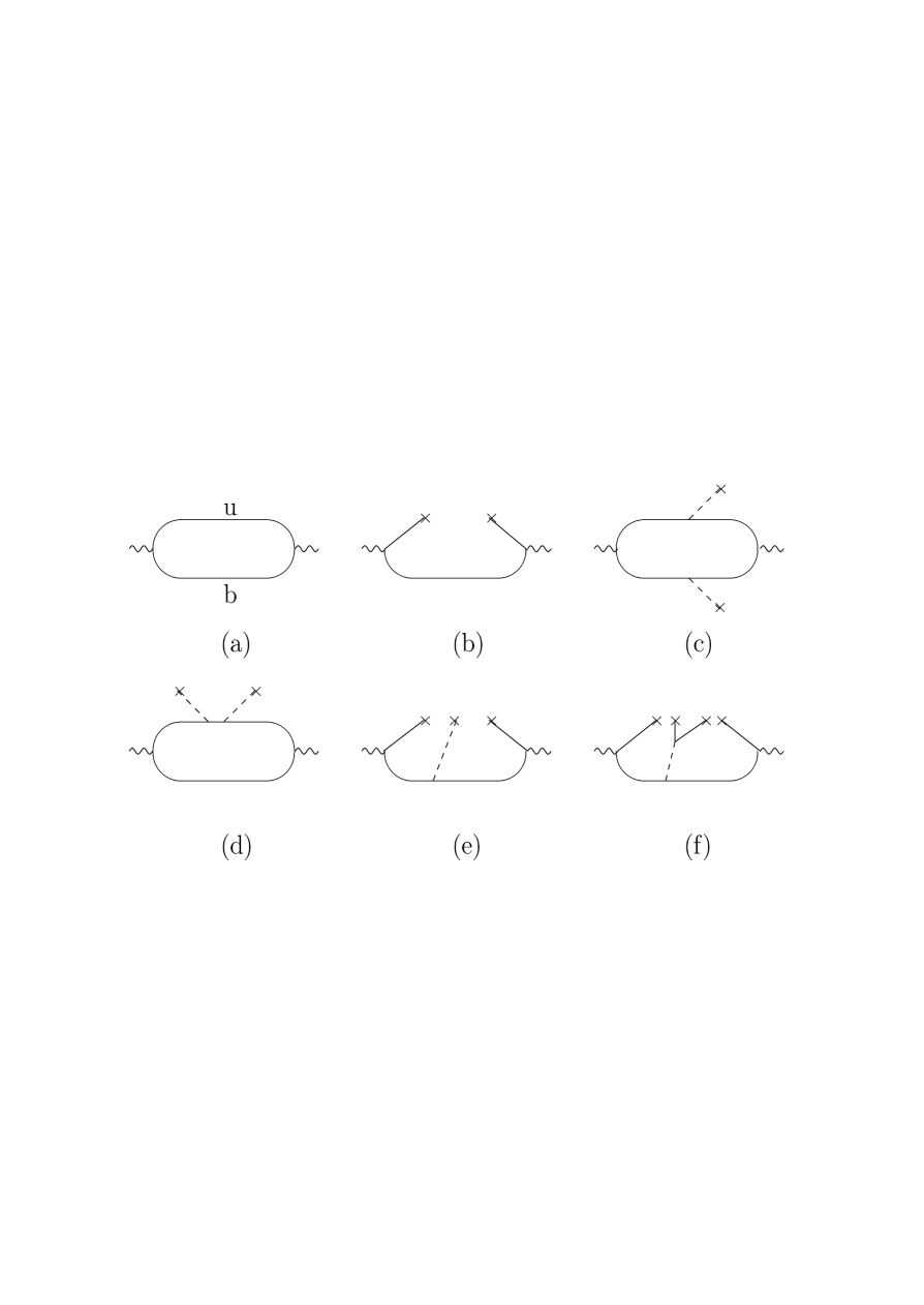
Figure 1: Diagrams determining the Wilson coefficients in the OPE of the two-point correlation function (2.4): $C_{0}$ (a), $C_{3}$ (b), $C_{4}$ (c,d), $C_{5}$ (b,e), $C_{6}$ (b,f). Solid lines denote quarks, dashed lines gluons, wavy lines external currents. Crosses indicate vacuum fields.

Figure 2: Feynman diagrams of the $O(\alpha_{s})$ correction to the Wilson coefficient $C_{0}(q^{2})$.

The complete result for the Borel-transformed correlation function (2.4) obtained in [11] is given by

$$\Pi(M^{2})=\frac{3}{8\pi^{2}}\int_{m_{b}^{2}}^{\infty}ds\frac{(s-m_{b}^{2})^{2}}{s}\left(1+\frac{4\alpha_{s}}{3\pi}f(s,m_{b}^{2})\right)\exp(-\frac{s}{M^{2}})$$

$$+\Bigg{(}-m_{b}\langle\bar{q}q\rangle+\frac{1}{12}\langle\frac{\alpha_{s}}{\pi}G^{a}_{\mu\nu}G^{a\mu\nu}\rangle-\frac{m_{b}}{2M^{2}}(1-\frac{m_{b}^{2}}{2M^{2}})m_{0}^{2}\langle\bar{q}q\rangle$$

$$-\frac{16\pi\alpha_{s}}{27M^{2}}(1-\frac{m_{b}^{2}}{4M^{2}}-\frac{m_{b}^{4}}{12M^{4}})\langle\bar{q}q\rangle^{2}\Bigg{)}\exp(-\frac{m_{b}^{2}}{M^{2}})~{},$$ (2.14)

where

$$f(s,m_{b}^{2})=\frac{9}{4}-2\int^{\frac{m_{b}^{2}}{s}}_{0}\frac{dt}{t}ln(1-t)+\ln\frac{s}{m_{b}^{2}}\ln\frac{s}{s-m_{b}^{2}}$$

$$+\frac{3}{2}\ln\frac{m_{b}^{2}}{s-m_{b}^{2}}+\ln\frac{s}{s-m_{b}^{2}}+\frac{m_{b}^{2}}{s}\ln\frac{s-m_{b}^{2}}{m_{b}^{2}}+\frac{m_{b}^{2}}{s-m_{b}^{2}}\ln\frac{s}{m_{b}^{2}}~{}.$$ (2.15)

The $b$-quark mass appearing in the perturbative contribution (first term in (2.14)) is defined to be the pole mass, while the choice of $m_{b}$ in the leading-order coefficients of the contributions from the higher-dimensional operators is arbitrary. Usually, the pole mass is used everywhere. In order to keep the formula readable, the scale dependence of the running coupling and the vacuum condensates is not made explicit in the above. Furthermore, use has been made of the conventional parametrization for the quark-gluon condensate density,

$$\langle\bar{q}\sigma_{\mu\nu}\frac{\lambda^{a}}{2}G^{a\mu\nu}q\rangle=m_{0}^{2}\langle\bar{q}q\rangle~{},$$ (2.16)

and of vacuum saturation reducing four-quark condensates to squares of quark condensates with known coefficients [2]:

$$\langle\bar{q}\Gamma_{r}q\bar{q}\Gamma_{s}q\rangle=\frac{1}{(12)^{2}}\{(Tr\Gamma_{r})(Tr\Gamma_{s})-Tr(\Gamma_{r}\Gamma_{s})\}\langle\bar{q}q\rangle^{2}~{}.$$ (2.17)

The two representations of $\Pi(M^{2})$, (2.11) and (2.14), yield an interesting equation which connects hadronic properties with QCD parameters. However, in order to determine the value of $f_{B}$ from it, one has to subtract the unknown contribution from the excited and continuum states to (2.11). In a reasonable approximation based on quark-hadron duality, one may estimate the integral over the hadronic spectral density $\rho^{h}$ by the corresponding integral over the perturbative density. This is achieved by substituting

$$\rho^{h}(s)\Theta(s-s_{0}^{h})=\frac{1}{\pi}\mbox{Im}C_{0}(s)\Theta(s-s_{0}^{B})$$ (2.18)

in (2.11), whereby $\sqrt{s_{0}^{B}}$ is treated as an effective threshold energy of the order of the mass of the first excited $B$ resonance. In this approximation, continuum subtraction amounts to a simple change of the upper limit of integration in (2.14) from $\infty$ to $s_{0}^{B}$. The uncertainty from this rough procedure should not be too harmful because of the suppression of excited and continuum states after Borel transformation.

Solving then the equation provided by (2.11) and (2.14) for $f_{B}$, one obtains the following sum rule:

$$f_{B}^{2}m_{B}^{4}=\frac{3m_{b}^{2}}{8\pi^{2}}\int_{m_{b}^{2}}^{s_{0}^{B}}ds\frac{(s-m_{b}^{2})^{2}}{s}\left(1+\frac{4\alpha_{s}}{3\pi}f(s,m_{b}^{2})\right)\exp\left(\frac{m_{B}^{2}-s}{M^{2}}\right)$$

$$+m_{b}^{2}\Bigg{\{}-m_{b}\langle\bar{q}q\rangle\left(1+\frac{m_{0}^{2}}{2M^{2}}\left(1-\frac{m_{b}^{2}}{2M^{2}}\right)\right)+\frac{1}{12}\langle\frac{\alpha_{s}}{\pi}G^{a}_{\mu\nu}G^{a\mu\nu}\rangle$$

$$-\frac{16\pi}{27}\frac{\alpha_{s}\langle\bar{q}q\rangle^{2}}{M^{2}}\left(1-\frac{m_{b}^{2}}{4M^{2}}-\frac{m_{b}^{4}}{12M^{4}}\right)\Bigg{\}}\exp\left(\frac{m_{B}^{2}-m_{b}^{2}}{M^{2}}\right)~{}.$$ (2.19)

Since the l.h.s. of this relation is a measurable quantity, any scale dependence on the r.h.s. must cancel, at least in principle. In practice, this can of course only be achieved approximately.

2.3 Numerical results

The numerical input in the sum rule (2.19) for $f_{B}$ is as follows. The pole mass of the $b$ quark is taken to be

$$m_{b}=4.7\pm 0.1~{}\mbox{GeV}~{},$$ (2.20)

covering the range of estimates obtained from bottomonium sum rules [12], while the continuum threshold in the $B$ channel is fixed to the range

$$s_{0}^{B}=35\mp 2~{}\mbox{GeV}^{2}~{}.$$ (2.21)

The scale $\mu$ at which $\alpha_{s}$ and the condensates are to be evaluated is still ambiguous in the approximation considered. A reasonable choice is

$$\mu^{2}=O(M^{2})$$ (2.22)

characterizing the average virtuality of the quarks in the correlator (2.4). Moreover, the products $m_{b}\langle\bar{q}q\rangle$ and $\langle\frac{\alpha_{s}}{\pi}G^{a}_{\mu\nu}G^{a\mu\nu}\rangle$ are renormalization-group invariant. Using the numerical value of the quark condensate density at $\mu=O(1~{}GeV)$ as derived from the PCAC relation [2, 13]:

$$\langle\bar{q}q\rangle(1~{}\mbox{GeV})=-\frac{f_{\pi}^{2}m_{\pi}^{2}}{2(m_{u}+m_{d})}\simeq-(240~{}\mbox{MeV})^{3}~{},$$ (2.23)

and the running mass $m_{b}(1GeV)$ corresponding to the central value (2.20) of the pole mass, one gets

$$m_{b}\langle\bar{q}q\rangle\simeq-0.084~{}\mbox{GeV}^{4}.$$ (2.24)

This is the estimate adopted for the present analysis together with the gluon condensate density determined from charmonium sum rules [2]:

$$\langle\frac{\alpha_{s}}{\pi}G^{a}_{\mu\nu}G^{a\mu\nu}\rangle\simeq 0.012~{}\mbox{GeV}^{4}~{}.$$ (2.25)

The remaining parameters are assumed to be

$$m_{0}^{2}(\mbox{1 GeV})\simeq 0.8~{}\mbox{GeV}^{2}$$ (2.26)

as extracted from sum rules for light baryons [14], and

$$\alpha_{s}\langle\bar{q}q\rangle^{2}=8\cdot 10^{-5}~{}\mbox{GeV}^{6}$$ (2.27)

as given in [11]. The scale dependence of $m_{0}^{2}\langle\bar{q}q\rangle$ and $\alpha_{s}\langle\bar{q}q\rangle^{2}$ is negligible. The numerical uncertainties in the condensate estimates vary from 10 % to about 50 % or more. They nevertheless play only a minor role for the total theoretical uncertainty on $f_{B}$.

Table 3: Decay constants of $B$ and $D$ mesons in MeV.

Method	Ref.	$f_{B}$	$f_{B_{s}}$	$f_{D}$	$f_{D_{s}}$
	$\stackrel{{\scriptstyle\mbox{this}}}{{\mbox{review}}}$	180 $\pm$ 30	–	190 $\pm$ 20	–
QCD sum rules
	[15] a)	175	210	$180\pm 10$	$220\pm 10$
	[16]	175$\pm$ 25	200$\pm$ 25	205$\pm$ 15	235 $\pm$ 15
Lattice	[17]	180$\pm$ 32	205$\pm$ 35	221$\pm$ 17	237$\pm$ 16
	[18]	$172^{+27}_{-31}$	$196^{+30}_{-35}$	$191^{+19}_{-28}$	$206^{+18}_{-28}$
	[7]	–	–	$<310$	–
Experiment
	[6] b)	–	–	–	241 $\pm$ 21$\pm$ 30

^a) update of results in [3, 11, 19] taking $m_{b}=4.67$ GeV, $s_{0}^{B}=35$ GeV²,
                  and $m_{c}=1.3$ GeV, $s_{0}^{D}=5.5$ GeV².
              ^b) world average

Next, one has to determine the range of values of the Borel parameter $M^{2}$ for which the sum rule (2.19) can be trusted. On the one hand, $M^{2}$ has to be small enough such that the contributions from excited and continuum states are exponentially damped and the approximation (2.18) is acceptable. On the other hand, the scale $M^{2}$ must be large enough such that higher-dimensional operators are suppressed and the OPE converges sufficiently fast. Furthermore, the sum rule should be stable under variations of $M^{2}$ in the allowed window. Whether or not these requirements can be met has to be investigated for each sum rule separately. In the case at hand, one finds that at

$$3~{}\mbox{GeV}^{2}\leq M^{2}\leq 5.5~{}\mbox{GeV}^{2}$$ (2.28)

the necessary conditions are fulfilled: the quark-gluon condensate contributes less than 15 %, and the four–quark operators a negligible amount, while the excited and continuum states contribute less than 30 %. Moreover, $f_{B}$ changes insignificantly when $M^{2}$ varies in the range (2.28).

The predictions on $f_{B}$ and $f_{B_{s}}$ derived from the sum rule (2.19) with the input specified above are summarized in Tab. 3 together with the corresponding results for $D$ mesons obtained with $m_{c}=1.3\pm 0.1$ GeV, $s_{0}^{D}=6\mp 1$ GeV², and 1 GeV${}^{2}<M^{2}<2$ GeV². The theoretical uncertainties are dominated by the uncertainties in the quark masses and continuum thresholds. For instance, the ranges of values of $f_{B}$ and $f_{D}$ expressed by the errors in the first row of Tab. 3 have been determined by varying $m_{Q}$ and $s_{0}^{P}$ simultaneously such that the stability of the sum rule is preserved. The correlation is indicated by the reversed $\pm$ sign in (2.21). It should also be emphasized that the $O(\alpha_{s})$ corrections have a sizeable effect. Without these corrections the decay constants would be considerably smaller:

$$\overline{f}_{B}\equiv f_{B}(\alpha_{s}=0)=140\pm 30~{}\mbox{MeV}~{},$$ (2.29)

$$\overline{f}_{D}\equiv f_{D}(\alpha_{s}=0)=170\pm 20~{}\mbox{MeV}~{}.$$ (2.30)

For comparison, Tab. 3 also shows recent lattice results and the available experimental data. The mutual agreement within the uncertainties of the two theoretical approaches is satisfactory. On the other hand, the data are just beginning to challenge theory.

3 Semileptonic decays and form factors

3.1 Distribution in momentum transfer

The weak hamiltonian (2.1) also applies to the semileptonic decay $B\to\pi\bar{l}\nu_{l}$. The appropriate hadronic matrix element is parametrized by two independent form factors:

$$\langle\pi(q)|\bar{u}\gamma_{\mu}b|B(p+q)\rangle=2f^{+}(p^{2})q_{\mu}+\left(f^{+}(p^{2})+f^{-}(p^{2})\right)p_{\mu}$$ (3.1)

with $p+q$, $q$ and $p$ being the $B$ and $\pi$ four-momenta, and the momentum transfer, respectively. Frequently, in particular in nonleptonic decays, one also uses the scalar form factor $f^{0}$ defined by

$$f^{0}(p^{2})=f^{+}(p^{2})+\frac{p^{2}}{m_{B}^{2}-m_{\pi}^{2}}f^{-}(p^{2})~{}.$$ (3.2)

The distribution of the momentum transfer squared in $B\to\pi\bar{l}\nu_{l}$ is given by

$$\frac{d\Gamma}{dp^{2}}=\frac{G^{2}|V_{ub}|^{2}}{24\pi^{3}}\frac{(p^{2}-m_{l}^{2})^{2}\sqrt{E_{\pi}^{2}-m_{\pi}^{2}}}{p^{4}m_{B}^{2}}\Bigg{\{}\left(1+\frac{m_{l}^{2}}{2p^{2}}\right)m_{B}^{2}(E_{\pi}^{2}-m_{\pi}^{2})\left[f^{+}(p^{2})\right]^{2}$$

$$+\frac{3m_{l}^{2}}{8p^{2}}(m_{B}^{2}-m_{\pi}^{2})^{2}\left[f^{0}(p^{2})\right]^{2}\Bigg{\}}~{},$$ (3.3)

where $E_{\pi}=(m_{B}^{2}+m_{\pi}^{2}-p^{2})/2m_{B}$ is the pion energy in the $B$ rest frame.

For $l=e,\mu$, the form factor $f^{0}$ plays a negligible role because of the smallness of the lepton masses. These channels can thus be used to directly determine the product $|V_{ub}f^{+}(p^{2})|$, while the heavy mode $B\to\pi\bar{\tau}\nu_{\tau}$ offers a possibility to test the scalar form factor $f^{0}(p^{2})$. Recently, the decays $B\to\pi\bar{l}\nu_{l}$ and $B\to\rho\bar{l}\nu_{l}$ have been observed by CLEO [20]. If the relevant form factors can be calculated with sufficient accuracy these measurements eventually provide interesting alternatives to the determination of $V_{ub}$ from inclusive $b\to u$ transitions. In these lectures, the sum rule method is advocated. It is one of the virtues of the sum rule calculations, in comparison to other approaches, that they can be tested and consistently improved by investigating the analogous $D$-meson form factors. The already existing experimental data on $D\to h\bar{l}\nu_{l}$, $h=K,K^{*},\pi,\rho,\eta$ and $l=e,\mu$ [21] have not yet been fully exploited in this respect.

3.2 Light-cone vs. short-distance expansion

For processes involving a light meson, e.g., a $\pi$, $K$, or $\rho$ there is an interesting alternative to the short-distance OPE of vacuum-vacuum correlation functions in terms of condensates, namely the expansion of vacuum-meson correlators near the light-cone in terms of meson wave functions [22, 23, 24]. The latter are defined by matrix elements of composite operators and classified by twist, similarly as the deep-inelastic structure functions. The light-cone variant of QCD sum rules has been suggested in [25, 26, 27]. In this approach, the light mesons are described by means of light-cone wave functions, whereas the heavy meson channels are treated in the usual way: choice of a generating current, dispersion relation, Borel transformation and continuum subtraction.

The general idea is explained in the following using the $B\rightarrow\pi$ matrix element (3.1) as an example. The detailed derivation of the light-cone sum rules for $f^{+}$ and $f^{-}$ is reported in [28, 29, 30] and reviewed in [5]. The central object is the vacuum-pion correlation function

$$F_{\mu}(p,q)=i\int d^{4}xe^{ipx}\langle\pi(q)\mid T\{\bar{u}(x)\gamma_{\mu}b(x),\bar{b}(0)i\gamma_{5}d(0)\}\mid 0\rangle$$ (3.4)

$$=F(p^{2},(p+q)^{2})q_{\mu}+\tilde{F}(p^{2},(p+q)^{2})p_{\mu}~{}.$$

From the comparison with (3.1) it is clear that the two invariant functions $F$ and $\tilde{F}$ have some kind of relation with the form factors $f^{+}$ and $f^{+}+f^{-}$, respectively. Since the pion is on-shell, $q^{2}=m_{\pi}^{2}$ vanishes in the chiral limit adopted throughout this discussion. For the momenta in the $\bar{b}d$ and $\bar{u}b$ channels one requires $(p+q)^{2}\ll m_{b}^{2}$ and $p^{2}\leq m_{b}^{2}-2m_{b}\chi$, $\chi$ being a $m_{b}$-independent scale of order $\Lambda_{QCD}$. This assures that the $b$ quark is far off mass-shell. Contracting the $b$-quark fields in (3.4) and inserting the free $b$-quark propagator, one gets

$$F_{\mu}(p,q) = i\int\frac{d^{4}x\,d^{4}k}{(2\pi)^{4}(m_{b}^{2}-k^{2})}e^{i(p-k)x}\left(m_{b}\langle\pi(q)|\bar{u}(x)\gamma_{\mu}\gamma_{5}d(0)|0\rangle\right.$$ (3.5)

$${}+\left.k^{\nu}\langle\pi(q)|\bar{u}(x)\gamma_{\mu}\gamma_{\nu}\gamma_{5}d(0)|0\rangle\right)~{}.$$

This contribution is diagrammaticly depicted in Fig. 3a. It is important to note that the path-ordered gluon operator

$$Pexp\left\{ig_{s}\int^{1}_{0}d\alpha~{}x_{\mu}A^{\mu}(\alpha x)\right\}$$ (3.6)

necessary for gauge invariance of the matrix elements in (3.5), is unity in the light-cone gauge, $x_{\mu}A^{\mu}=0$, assumed here.

Figure 3: Diagrammatic representation of the correlation function (3.4): terms involving two-particle (a) and three-particle (b) wave functions. Solid lines represent quarks, dashed lines gluons, wavy lines external currents, and ovals light-cone wave functions of the pion.

Let us first consider the matrix element

$$\langle\pi(q)|\bar{u}(x)\gamma_{\mu}\gamma_{5}d(0)|0\rangle,$$ (3.7)

and expand the bilocal quark-antiquark operator around $x=0$:

$$\bar{u}(x)\gamma_{\mu}\gamma_{5}d(0)=\sum_{r}\frac{1}{r!}\bar{u}(0)(\stackrel{{\scriptstyle\leftarrow}}{{D}}\cdot x)^{r}\gamma_{\mu}\gamma_{5}d(0)~{}.$$ (3.8)

The matrix elements of the local operators can be written in the form

$$\langle\pi(q)|\bar{u}\stackrel{{\scriptstyle\leftarrow}}{{D}}_{\alpha_{1}}\stackrel{{\scriptstyle\leftarrow}}{{D}}_{\alpha_{2}}...\stackrel{{\scriptstyle\leftarrow}}{{D}}_{\alpha_{r}}\gamma_{\mu}\gamma_{5}d|0\rangle=(i)^{r}q_{\mu}q_{\alpha_{1}}q_{\alpha_{2}}...q_{\alpha_{r}}M_{r}+...~{},$$ (3.9)

where the ellipses stand for additional terms containing the metric tensor $g_{\alpha_{i}\alpha_{k}}$ in all possible combinations. Note that the lowest twist in (3.9) is equal to 2. Substituting (3.8) and (3.9) in the first term of (3.5), integrating over $x$ and $k$, and comparing the result with (3.4), one obtains

$$F(p^{2},(p+q)^{2})=i\frac{m_{b}}{m_{b}^{2}-p^{2}}\sum_{r=0}^{\infty}\xi^{r}M_{r}~{}$$ (3.10)

with

$$\xi=\frac{2(p\cdot q)}{m_{b}^{2}-p^{2}}=\frac{(p+q)^{2}-p^{2}}{m_{b}^{2}-p^{2}}~{}.$$ (3.11)

Obviously, if the ratio $\xi$ is finite one must keep an infinite series of matrix elements in (3.10). All of them give contributions of the same order in the heavy quark propagator $1/(m_{b}^{2}-p^{2})$, differing only by powers of the dimensionless parameter $\xi$. In other words, the expansion (3.8) is useful only in the case $\xi\rightarrow 0$, i.e., $p^{2}\rightarrow(p+q)^{2}$ or equivalently, when the pion momentum vanishes. In this case, the series in (3.10) can be truncated after a few terms involving only a manageable number of unknown matrix elements $M_{r}$. However, generally, when $p^{2}\neq(p+q)^{2}$ one has to sum up the infinite series of matrix elements of local operators in some way.

One possible solution of this problem is provided by the light-cone expansion of the bilocal operator (3.8). For the matrix element (3.7) the first term of this expansion is given by

$$\langle\pi(q)|\bar{u}(x)\gamma_{\mu}\gamma_{5}d(0)|0\rangle_{x^{2}=0}=-iq_{\mu}f_{\pi}\int_{0}^{1}du\,e^{iuqx}\varphi_{\pi}(u)~{}.$$ (3.12)

The function $\varphi_{\pi}(u)$ is known as the twist 2 light-cone wave function of the pion. It represents the distribution in the fraction of the light-cone momentum $q_{0}+q_{3}$ of the pion carried by a constituent quark. As can be seen by putting $x=0$ in the above, $\varphi_{\pi}(u)$ is normalized to unity. Substitution of (3.12) in (3.5) and integration over $x$ and $k$ yields

$$F(p^{2},(p+q)^{2})=m_{b}f_{\pi}\int_{0}^{1}\frac{du~{}\varphi_{\pi}(u)}{m_{b}^{2}-(p+uq)^{2}}~{}.$$ (3.13)

We see that the infinite series of matrix elements of local operators encountered before in (3.10) is effectively replaced by a wave function. Formal expansion of (3.13) in $q$,

$$F(p^{2},(p+q)^{2})=m_{b}f_{\pi}\sum_{r=0}^{\infty}\frac{(2p\cdot q)^{r}}{(m_{b}^{2}-p^{2})^{r+1}}\int_{0}^{1}du~{}u^{r}\varphi_{\pi}(u)~{},$$ (3.14)

and comparison with (3.10) yields the relation between the matrix elements $M_{r}$ defined in (3.9) and the moments of $\varphi_{\pi}(u)$:

$$M_{r}=-if_{\pi}\int_{0}^{1}du~{}u^{r}\varphi_{\pi}(u).$$ (3.15)

Including the next-to-leading terms in $x^{2}$, the light-cone expansion of the matrix element (3.7) is given by

$$\langle\pi(q)|\bar{u}(x)\gamma_{\mu}\gamma_{5}d(0)|0\rangle=-iq_{\mu}f_{\pi}\int_{0}^{1}du\,e^{iuqx}\left(\varphi_{\pi}(u)+x^{2}g_{1}(u)\right)$$

$$+f_{\pi}\left(x_{\mu}-\frac{x^{2}q_{\mu}}{qx}\right)\int_{0}^{1}du\,e^{iuqx}g_{2}(u),$$ (3.16)

where $g_{1}$ and $g_{2}$ are twist 4 wave functions. Proceeding to the second term in (3.5) and using the relation

$$\gamma_{\mu}\gamma_{\nu}\gamma_{5}=g_{\mu\nu}\gamma_{5}-i\sigma_{\mu\nu}\gamma_{5}~{},$$ (3.17)

one encounters two further matrix elements:

$$\langle\pi(q)\mid\bar{u}(x)i\gamma_{5}d(0)\mid 0\rangle=f_{\pi}\mu_{\pi}\int_{0}^{1}du~{}e^{iuqx}\varphi_{p}(u)$$ (3.18)

and

$$\langle\pi(q)\mid\bar{u}(x)\sigma_{\mu\nu}\gamma_{5}d(0)\mid 0\rangle=i(q_{\mu}x_{\nu}-q_{\nu}x_{\mu})\frac{f_{\pi}\mu_{\pi}}{6}\int_{0}^{1}du~{}e^{iuqx}\varphi_{\sigma}(u)\,$$ (3.19)

with $\mu_{\pi}=m_{\pi}^{2}/(m_{u}+m_{d})$. Only the leading terms of the expansion are considered here. They have twist 3 and are parameterized by the wave functions $\varphi_{p}$ and $\varphi_{\sigma}$.

Beyond twist 2, one should also take into account the higher-order term illustrated graphically in Fig. 3b, where a gluon is emitted from the heavy quark line. This correction is determined by quark-antiquark-gluon wave functions [31]. Explicit expressions for this contribution can be found in [28, 29] and also in [5]. Below, this term is denoted by $F_{G}$. Gluon radiation from the light quark lines in Fig. 3a is effectively included in the twist 3 and 4 wave functions as was shown in [26, 32, 33]. Components of the pion wave function with two extra gluons, or with an additional $\bar{q}q$ pair are neglected. Including all operators up to twist 4 one obtains the following results for the two invariant functions defined in (3.4):

$$F(p^{2},(p+q)^{2}) = f_{\pi}\int\limits_{0}^{1}\frac{du}{m_{b}^{2}-(p+uq)^{2}}\Bigg{\{}m_{b}\varphi_{\pi}(u)$$ (3.20)

$${}+\mu_{\pi}\Bigg{[}u\varphi_{p}(u)+\frac{1}{6}\left(2+\frac{p^{2}+m_{b}^{2}}{m_{b}^{2}-(p+uq)^{2}}\right)\varphi_{\sigma}(u)\Bigg{]}$$

$${}+m_{b}\left[\frac{2ug_{2}(u)}{m_{b}^{2}-(p+uq)^{2}}-\frac{8m_{b}^{2}}{(m_{b}^{2}-(p+uq)^{2})^{2}}\left(g_{1}(u)-\int^{u}_{0}dvg_{2}(v)\right)\right]\Bigg{\}}$$

$${}+F_{G}(p^{2},(p+q)^{2})$$

$$\widetilde{F}(p^{2},(p+q)^{2}) = f_{\pi}\int\limits_{0}^{1}\frac{du}{m_{b}^{2}-(p+uq)^{2}}\Bigg{\{}\mu_{\pi}\varphi_{p}(u)+\frac{\mu_{\pi}\varphi_{\sigma}(u)}{6u}$$ (3.21)

$${}\times\Bigg{[}1-\frac{m_{b}^{2}-p^{2}}{m_{b}^{2}-(p+uq)^{2}}\Bigg{]}+\frac{2m_{b}g_{2}(u)}{m_{b}^{2}-(p+uq)^{2}}\Bigg{\}}~{}.$$

We see that every power of $x^{2}$ in the light-cone expansion of the integrand in (3.4) leads to an additional power of $m_{b}^{2}-(p+uq)^{2}$ in the denominators of the coefficients. This justifies the neglect of higher-twist operators, provided $(p+q)^{2}$ and $p^{2}$ are sufficiently smaller than $m_{b}^{2}$. It is also interesting to note that there are no contributions from twist 2 and from three-particle wave functions to $\tilde{F}$.

3.3 Light-cone wave functions

Before proceeding with the derivation of the light-cone sum rules for the form factors $f^{\pm}$, it may be useful to make a few more remarks on the light-cone wave functions. Firstly, these functions are universal, a property which is essential for the whole approach, similarly as the universality of the vacuum condensates in the case of short-distance sum rules. Secondly, the asymptotic form of the wave functions is given by conformal symmetry and asymptotic freedom of QCD [24, 33], while the nonasymptotic features incorporate long-distance quark-gluon interactions. Thirdly, the factorization of collinear logarithms generated by gluon radiation and the renormalization procedure induce scale dependences. Usually, a common scale $\mu$ is chosen for simplicity.

In leading-order approximation (LO), the twist 2 wave function $\varphi_{\pi}(u,\mu)$ obeys the Brodsky-Lepage evolution equation [22]:

$$\frac{d\varphi_{\pi}(u,\mu)}{d\ln\mu}=\int\limits_{0}^{1}dwV(u,w)\varphi_{\pi}(w,\mu)~{},$$ (3.22)

where

$$V(u,w)=\frac{\alpha_{s}(\mu)C_{F}}{\pi}\left[\frac{1-u}{1-w}\left(1+\frac{1}{u-w}\right)\Theta(u-w)+\frac{u}{w}\left(1+\frac{1}{w-u}\right)\Theta(w-u)\right]_{+}$$ (3.23)

and the $+$ regularization is defined by

$$R(u,w)_{+} = R(u,w)-\delta(u-w)\int\limits_{0}^{1}R(v,w)dv~{}.$$ (3.24)

The evolution equation effectively sums up the leading logarithms to all orders. It can be solved by expanding $\varphi_{\pi}(u,\mu)$ in terms of Gegenbauer polynomials

$$\varphi_{\pi}(u,\mu)=6u(1-u)\Big{[}1+\sum_{i}a_{2i}(\mu)C^{3/2}_{2i}(2u-1)\Big{]}\,,$$ (3.25)

in which case the coefficients $a_{2i}(\mu)$ are multiplicatively renormalizable [22]. The scale dependence is given by

$$a_{n}(\mu)=a_{n}(\mu_{0})\left(\frac{\alpha_{s}(\mu)}{\alpha_{s}(\mu_{0})}\right)^{\gamma_{n}/b}~{},$$ (3.26)

where $b=11-2n_{f}/3$ is the 1-loop coefficient of the QCD beta function, $n_{f}$ being the number of active flavours, and

$$\gamma_{n}=C_{F}\left[-3-\frac{2}{(n+1)(n+2)}+4\left(\sum_{k=1}^{n+1}\frac{1}{k}\right)\right]$$ (3.27)

are the anomalous dimensions [24]. We see that $a_{n}(\mu)$, $n\geq 2$ vanishes for $\mu\rightarrow\infty$. Therefore, these terms describe the nonasymptotic effects in the wave function (3.25). The $\mu$-independent term is the asymptotic wave function, $\varphi_{\pi}(u,\mu=\infty)=6u(1-u)$. As already pointed out, the normalization is such that

$$\int^{1}_{0}du\varphi_{\pi}(u,\mu)=1~{}.$$ (3.28)

The initial values of the nonasymptotic coefficients can be estimated from two-point sum rules [24] for the moments $\int u^{n}\varphi_{\pi}(u,\mu)du$ at low $n$. The nonperturbative information encoded in the quark and gluon condensates is thereby transmuted into the long-distance properties of the wave function. Alternatively, one can determine the coefficients directly from light-cone sum rules for known hadronic quantities such as the $\pi NN$ and $\omega\rho\pi$ couplings. Here, the estimates at $\mu_{0}=0.5$ GeV given in [26] are adopted:

$$a_{2}(\mu_{0})=\frac{2}{3},~{}a_{4}(\mu_{0})=0.43~{}.$$ (3.29)

The corresponding Gegenbauer polynomials are given by

$$C_{2}^{3/2}(2u-1) = \frac{3}{2}[5(2u-1)^{2}-1]~{},$$

$$C_{4}^{3/2}(2u-1) = \frac{15}{8}[21(2u-1)^{4}-14(2u-1)^{2}+1]~{}.$$ (3.30)

On the basis of the approximate conformal symmetry of QCD it has been shown [33] that the expansion (3.25) converges sufficiently fast so that the terms with $n>4$ are negligible.

For completeness, the twist 3 and 4 two-particle light-cone wave functions of the pion are listed below [24, 26]:

$$\varphi_{p}(u,\mu) = 1+B_{2}(\mu)\frac{1}{2}(3(u-\bar{u})^{2}-1)+B_{4}(\mu)\frac{1}{8}(35(u-\bar{u})^{4}$$ (3.31)

$${}-30(u-\bar{u})^{2}+3)~{},$$

$$\varphi_{\sigma}(u,\mu) = 6u\bar{u}\Big{[}1+C_{2}(\mu)\frac{3}{2}(5(u-\bar{u})^{2}-1)$$ (3.32)

$${}+C_{4}(\mu)\frac{15}{8}(21(u-\bar{u})^{4}-14(u-\bar{u})^{2}+1)\Big{]}~{},$$

$$g_{1}(u,\mu) = \frac{5}{2}\delta^{2}(\mu)\bar{u}^{2}u^{2}+\frac{1}{2}\varepsilon(\mu)\delta^{2}(\mu)[\bar{u}u(2+13\bar{u}u)+10u^{3}\ln u(2-3u+\frac{6}{5}u^{2})$$ (3.33)

$${}+10\bar{u}^{3}\ln\bar{u}(2-3\bar{u}+\frac{6}{5}\bar{u}^{2})]~{},$$

$$g_{2}(u,\mu) = \frac{10}{3}\delta^{2}(\mu)\bar{u}u(u-\bar{u})~{},$$ (3.34)

$$\int\limits_{0}^{u}dvg_{2}(v,\mu) = \frac{5}{3}\delta^{2}(\mu)\bar{u}^{2}u^{2}$$ (3.35)

with $\bar{u}=1-u$ and

$$B_{2}=30\frac{f_{3\pi}}{\mu_{\pi}f_{\pi}}\,,~{}~{}B_{4}=\frac{3}{2}\frac{f_{3\pi}}{\mu_{\pi}f_{\pi}}(4\omega_{2,0}-\omega_{1,1}-2\omega_{1,0})\,,$$

$$C_{2}=\frac{f_{3\pi}}{\mu_{\pi}f_{\pi}}(5-\frac{1}{2}\omega_{1,0})\,,~{}~{}C_{4}=\frac{1}{10}\frac{f_{3\pi}}{\mu_{\pi}f_{\pi}}(4\omega_{2,0}-\omega_{1,1})~{}.$$ (3.36)

The additional parameters appearing in the above are numerically given by

$$f_{3\pi}(1\mbox{GeV})=0.0035~{}\mbox{\rm GeV}^{2}~{},$$

$$\omega_{1,0}(1\mbox{GeV})=-2.88\,,~{}~{}\omega_{2,0}(1\mbox{GeV})=10.5\,,~{}~{}\omega_{1,1}(1\mbox{GeV})=0\,,$$

$$\delta^{2}(1\mbox{GeV})=0.2~{}\mbox{GeV}^{2}\,,~{}~{}\varepsilon(1\mbox{GeV})=0.5~{}.$$ (3.37)

For the quark-antiquark-gluon wave functions the reader is referred to [31] and [5].

3.4 Sum rules for heavy-to-light form factors

Now we are ready to proceed with the discussion of the $B\to\pi$ transition form factors. In order to determine $f^{\pm}(p^{2})$ from the correlation function $F_{\mu}(p,q)$ derived in (3.4), we apply QCD sum rule methods to the $B$-meson channel following essentially the same steps as in the derivation of the sum rule for $f_{B}$ in sect. 2.2. The hadronic representation of (3.4) is obtained by inserting a complete set of intermediate states with $B$-meson quantum numbers between the currents on the r.h.s. of (3.4). Using the matrix elements (2.5) and (3.1), and representing the sum over excited and continuum states by a dispersion integral with the spectral density $\rho^{h}_{\mu}=\rho^{h}q_{\mu}+\tilde{\rho}^{h}p_{\mu}$, one obtains the following relations for the invariant amplitudes $F$ and $\tilde{F}$:

$$F(p^{2},(p+q)^{2})=\frac{2m_{B}^{2}f_{B}f^{+}(p^{2})}{m_{b}(m_{B}^{2}-(p+q)^{2})}+\int\limits_{s_{0}^{h}}^{\infty}\frac{\rho^{h}(p^{2},s)ds}{s-(p+q)^{2}}~{},$$ (3.38)

$$\widetilde{F}(p^{2},(p+q)^{2})=\frac{m_{B}^{2}f_{B}(f^{+}(p^{2})+f^{-}(p^{2}))}{m_{b}(m_{B}^{2}-(p+q)^{2})}+\int\limits_{s_{0}^{h}}^{\infty}ds\frac{\tilde{\rho}^{h}(p^{2},s)}{s-(p+q)^{2}}~{}.$$ (3.39)

Similarly as in (2.11), the integrals over $\rho^{h}$ and $\tilde{\rho}^{h}$ are approximated by corresponding integrals over the spectral densities calculated from the light-cone expansion of (3.4) using the substitution

$$\rho^{h}(p^{2},s)\Theta(s-s_{0}^{h})=\frac{1}{\pi}\mbox{Im}F(p^{2},s)\Theta(s-s_{0}^{B})~{},$$ (3.40)

and the analogous relation for $\tilde{\rho}_{h}$ and $\mbox{Im}\tilde{F}$. The calculation of the imaginary parts of $F$ and $\tilde{F}$ from the functions given in (3.20) and (3.21), respectively, is outlined, e.g., in [5]. With the above duality approximation it is again rather straightforward to subtract the continuum contributions from the l.h.s. of (3.38) and (3.39). After performing the Borel transformation in $(p+q)^{2}$, one arrives at the sum rules [28, 29]

$$f_{B}f^{+}(p^{2})=\frac{f_{\pi}m_{b}^{2}}{2m_{B}^{2}}\exp\left(\frac{m_{B}^{2}}{M^{2}}\right)\Bigg{\{}\int\limits_{\Delta}^{1}\frac{du}{u}exp\left[-\frac{m_{b}^{2}-p^{2}(1-u)}{uM^{2}}\right]$$

$$\times\Bigg{(}\varphi_{\pi}(u)+\frac{\mu_{\pi}}{m_{b}}\Bigg{[}u\varphi_{p}(u)+\frac{\varphi_{\sigma}(u)}{3}\left(1+\frac{m_{b}^{2}+p^{2}}{2uM^{2}}\right)\Bigg{]}$$

$$-\frac{4m_{b}^{2}g_{1}(u)}{u^{2}M^{4}}+\frac{2}{uM^{2}}\int\limits_{0}^{u}g_{2}(v)dv\left(1+\frac{m_{b}^{2}+p^{2}}{uM^{2}}\right)\Bigg{)}+t^{+}(s_{0}^{B},p^{2},M^{2})$$

$$+f^{+}_{G}(p^{2},M^{2})+\frac{\alpha_{s}C_{F}}{4\pi}\delta^{+}(p^{2},M^{2})\Bigg{\}}~{},$$ (3.41)

and [30]

$$f_{B}(f^{+}(p^{2})+f^{-}(p^{2}))=\frac{f_{\pi}\mu_{\pi}m_{b}}{m_{B}^{2}}\exp\left(\frac{m_{B}^{2}}{M^{2}}\right)\Bigg{\{}\int\limits_{\Delta}^{1}\frac{du}{u}\exp\left[-\frac{m_{b}^{2}-p^{2}(1-u)}{uM^{2}}\right]$$

$$\times\Bigg{[}\varphi_{p}(u)+\frac{\varphi_{\sigma}(u)}{6u}\left(1-\frac{m_{b}^{2}-p^{2}}{uM^{2}}\right)+\frac{2m_{b}g_{2}(u)}{\mu_{\pi}uM^{2}}\Bigg{]}+t^{\pm}(s_{0}^{B},p^{2},M^{2})\Bigg{\}}~{}.$$ (3.42)

The sum rule for the scalar form factor $f^{0}$ follows from the relation (3.2). In the above, $t^{+}$ and $t^{\pm}$ are numerically small corrections left from continuum subtraction, and $f^{+}_{G}$ denotes the contribution from the three-particle wave functions. The explicit expressions of these terms are given in [29, 30]. Also indicated is the perturbative QCD correction $\delta^{+}$ to the leading twist 2 term in $f^{+}$ which has been calculated only recently [34, 35]. Other perturbative corrections are still unknown.

Concerning the $O(\alpha_{s})$ correction to the leading twist 2 result, a few comments are in order. Hard gluon exchanges give rise to radiative effects in the correlation function (3.4) which can be calculated perturbatively. The first-order diagrams are shown in Fig. 4. The expression (3.13) of the invariant function $F$ can be more generally written as a convolution of a hard scattering amplitude $T$ with the twist 2 wave function:

$$F(p^{2},(p+q)^{2})=f_{\pi}\int^{1}_{0}du\varphi_{\pi}(u,\mu)T(p^{2},(p+q)^{2},u,\mu)~{},$$ (3.43)

where $T$ is determined by a perturbative series

$$T(p^{2},(p+q)^{2},u,\mu)=T_{0}(p^{2},(p+q)^{2},u)+\frac{\alpha_{s}C_{F}}{4\pi}T_{1}(p^{2},(p+q)^{2},u,\mu)+O(\alpha_{s}^{2})~{}.$$ (3.44)

Figure 4: Diagrams of the $O(\alpha_{s})$ corrections to the correlation function (3.4).

The LO approximation is given by the zero-order amplitude

$$T_{0}(p^{2},(p+q)^{2},u)=\frac{m_{b}}{m_{b}^{2}-p^{2}(1-u)-(p+q)^{2}u}$$ (3.45)

convoluted with the wave function obeying the LO Brodsky-Lepage evolution equation (3.22). In next-to-leading order (NLO), the hard amplitude (3.44) includes the first-order term $T_{1}$, while the wave function $\varphi_{\pi}(u,\mu)$ solves the NLO evolution equation [36]. For calculational details and analytic results one may consult [34, 35]. To date, the NLO program is completed only for the twist 2 contribution to the invariant amplitude $F$.

It is important to note that the correlation function (3.4) actually leads to sum rules for products of decay constants and form factors as made explicit in (3.41) and (3.42). When dividing out the decay constants, consistency requires to take both the sum rule and $f_{P}$ in LO or in NLO. This appears obvious, but has not always been respected in the literature. Some of the discrepancies in the calculations originate just from mixing orders. In fact, as will be quantified later, the remaining radiative corrections to $f^{+}(p^{2})$ turn out to be rather small because of a cancellation of the corrections to the sum rules (3.41) for $f_{B}f^{+}(p^{2})$ and (2.19) for $f_{B}$.

As a final remark, the light-cone sum rules provide a unique possibility to investigate the heavy-mass dependence of the heavy-to-light form factors. To this end, one employs the following scaling relations for mass parameters and decay constants:

$$m_{P}=m_{Q}+\bar{\Lambda}~{},~{}~{}~{}s_{0}^{P}=m_{Q}^{2}+2m_{Q}\omega_{0}~{},~{}~{}~{}M^{2}=2m_{Q}\tau~{},$$ (3.46)

$$f_{p}=\hat{f}_{P}/\sqrt{m_{Q}},$$ (3.47)

where in the heavy quark limit $\bar{\Lambda}$, $\omega_{0}$, $\tau$, $\hat{f}_{P}$ are $m_{Q}$-independent quantities. With these substitutions it is straightforward to expand the sum rules (3.41) and (3.42) in $m_{Q}$. In both cases, the light-cone expansion in terms of wave functions with increasing twist is consistent with the heavy mass expansion, that is the higher-twist contributions either scale with the same power of $m_{Q}$ as the leading-twist term, or they are suppressed by extra powers of $m_{Q}$.

The asymptotic scaling behaviour of the form factors turns out to differ sharply at small and large momentum transfer [30]. At $p^{2}=0$

$$f^{+}(0)=f^{0}(0)\sim m_{Q}^{-3/2}~{},$$ (3.48)

$$f^{+}(0)+f^{-}(0)\sim m_{Q}^{-3/2}~{},$$ (3.49)

whereas at $p^{2}=m_{Q}^{2}-2m_{Q}\chi$, $\chi$ being independent of $m_{Q}$,

$$f^{+}(p^{2})\sim m_{Q}^{1/2}~{},$$ (3.50)

$$f^{+}(p^{2})+f^{-}(p^{2})\simeq f^{0}(p^{2})\sim m_{Q}^{-1/2}~{}.$$ (3.51)

The sum rules thus nicely reproduce the asymptotic dependence of the form factors on the heavy quark mass derived in [37, 38] for small pion momentum in the rest frame of the $P$ meson. In addition, the sum rules allow to investigate the opposite region of large pion momentum where neither HQET nor the single-pole model can be trusted. Clearly, from the sum rule point of view it is expected that the excited and continuum states become more and more important as $p^{2}\rightarrow 0$. This is reflected in the change of the asymptotic mass dependence. Claims in the literature which differ from (3.48) to (3.51) are often based on the pole model and therefore not reliable. A similar analysis has been carried out in [39] for $B\rightarrow\rho$ form factors with essentially the same conclusions.

3.5 Numerical analysis

For most of the following illustrations, it suffices to work in LO. Strictly speaking, since the NLO order corrections to $f_{B}(f^{+}+f^{-})$ are unknown, it is also more consistent to work in LO when combining or comparing $f^{+}$ and $f^{+}+f^{-}$. Therefore, if not stated otherwise, the values of $m_{b}$, $s_{0}^{B}$, and $f_{B}(\alpha_{s}=0)$ specified in (2.20), (2.21) and (2.29), respectively, are used. The pion wave functions are as given in sect. 3.3 with the coefficients scaled to

$$\mu_{b}=\sqrt{m_{B}^{2}-m_{b}^{2}}\simeq 2.4\,\mbox{\rm GeV}~{}.$$ (3.52)

With this input we have checked that for $M^{2}=10\pm 2$ GeV² the twist 4 corrections are very small, and that the continuum contributions do not exceed $30\%$. Up to $p^{2}\simeq 18$ GeV², the sum rules are also quite stable under variation of $M^{2}$. At larger momentum transfer the sum rules become unstable, and the twist 4 contribution grows rapidly. This is not surprising because the light-cone expansion and the sum rule method are expected to break down as $p^{2}$ approaches $m_{b}^{2}$.

Figure 5: $B\to\pi$ form factors obtained from light-cone sum rules in LO.

The momentum dependence of the form factors $f^{+}$ and $f^{+}+f^{-}$ can be seen in Fig. 5. Specifically, at zero momentum transfer we predict

$$f^{+}(0)=0.30,$$

$$f^{+}(0)+f^{-}(0)=0.06.$$ (3.53)

If the known $O(\alpha_{s})$ corrections are included in the sum rules for $f_{B}f^{+}(p^{2})$ and $f_{B}$, one gets instead

$$f^{+}(0)=0.27.$$ (3.54)

Figure 6: Variation of the sum rule prediction on $f^{+}(p^{2})$ with the Borel parameter (a), the $b$-quark mass (b), and the continuum threshold $s_{0}^{B}$ (c). Considered are three typical values of momentum transfer: $p^{2}=0$ (solid), $p^{2}=8$ GeV² (long-dashed), and $p^{2}=16$ GeV² (short-dashed).

Allowing the parameters to vary within the ranges specified one can estimate the uncertainties in the sum rule predictions. The main sources of uncertainty are discussed below:

(a) Borel mass parameter

The dependence of $f^{+}$ on $M^{2}$ is illustrated in Fig. 6a. In the allowed interval of $M^{2}$, $f^{+}$ deviates by only $\pm$(3 to 5) % from the nominal value, depending slightly on $p^{2}$.

(b) $b$-quark mass and continuum threshold

Fig. 6b shows the variation of $f^{+}$ with $m_{b}$ keeping all other parameters except $f_{B}$ fixed. The value of $f_{B}$ is taken from the sum rule (2.19) after dropping the $O(\alpha_{s})$ corrections. The analogous test for $s_{0}^{B}$ is performed in Fig. 6c. If $s_{0}^{B}$ and $m_{b}$ are varied simultaneously such that one achieves maximum stability of the sum rule for $f_{B}$, the change in $f^{+}$ is negligible at small $p^{2}$ and only about $\pm$ 3 % at large $p^{2}$.

Figure 7: $B\to\pi$ form factor $f^{+}$: (a) individual contributions of twist 2 (dashed), 3 (dash-dotted), and 4 (dotted), and the total sum (solid); (b) wave functions with (solid) and without (dashed) nonasymptotic corrections.

(c) higher-twist contributions

No reliable estimates exist for wave functions beyond twist 4. Therefore, we use the magnitude of the twist 4 contribution to $f^{+}$ as an indicator for the uncertainty due to the neglect of higher-twist terms. From Fig. 7a we see that the impact of the twist 4 components is comfortably small, less than 2 % at low $p^{2}$ and about 5 % at large $p^{2}$. This suggests a conservative estimate of $\pm$ 5 % uncertainty due to unknown higher-twist.

(d) light-cone wave functions

In order to clarify the sensitivity of $f^{+}$ to the nonasymptotic effects in the wave functions, the corresponding coefficients are put to zero and the result is compared, in Fig. 7b, to the nominal prediction. The change amounts to about -10 % at small $p^{2}$ and +10 % at large $p^{2}$, while the intermediate region around $p^{2}\simeq 10$ GeV² is very little affected. Since this exercise is rather extreme, the real uncertainty from the errors in the nonasymptotic coefficients is considerably smaller.

Figure 8: $B\to\pi$ form factor $f^{+}(p^{2})$ in leading twist 2 approximation: LO (dashed) in comparison to NLO (solid).

(e) perturbative corrections

The $O(\alpha_{s})$ corrections to the leading twist 2 term in the sum rule (3.41) for $f_{B}f^{+}$ and to the sum rule (2.19) for $f_{B}$, both being about 30 %, cancel in the ratio. The net effect is the surprisingly small correction to $f^{+}$ shown in Fig. 8. This result [34, 35] eliminates one main uncertainty. Unfortunately, the perturbative corrections to the higher-twist terms are not known. Considering that the twist 3 terms contribute about 50 % to the sum rule for $f_{B}f^{+}$, and assuming again radiative corrections of about 30 % but no cancellation, the remaining uncertainty is 15 %.

In summary, the present total uncertainty in the normalization of $f^{+}(p^{2})$ is estimated to be about 25 %, if the individual contributions (a) to (e) with the exception of (d) are added up linearly, and about 17 % if they are added in quadrature as is often done in the literature. Ultimately, this may be reduced to about 15 to 10 %. In addition, there is a shape-dependent uncertainty from (d) of less than -10 % at low and +10 % at high $p^{2}$. Moreover, in the integrated width the latter uncertainty averages out almost completely. The uncertainties from (a) to (d) on $f^{+}+f^{-}$ are of comparable size, while the effect of radiative corrections is still unknown.

Finally, it is interesting to compare the predictions on the $B\rightarrow\pi$ form factors from the light-cone sum rules with the results of other approaches. Such a comparison is presented in Fig. 9 and 10. Although there is rough agreement on the normalization at low momentum transfer, the light-cone sum rules predict the fastest increase of $f^{+}$ with $p^{2}$.

Figure 9: $B\to\pi$ form factor $f^{+}$ calculated in different approaches: three-point sum rule [40] (dashed), quark model [41] (dotted), and light-cone sum rule [28, 30] (solid).

Figure 10: The $B\rightarrow\pi$ form factor $f^{0}$: light-cone sum rule prediction (solid) in comparison to the quark model result from [41] (dashed) and the sum rule estimate from [42] (dash-dotted).

The sum rules (3.41) and (3.42) for the $B\rightarrow\pi$ form factors are formally converted into sum rules for the $D\rightarrow\pi$ form factors by replacing $b$ with $c$ and $B$ with $D$. The input parameters are taken over from the calculation of $f_{D}$ in sect. 2.2. In addition, one has to rescale the wave functions from $\mu_{b}\simeq 2.4$ GeV to $\mu_{c}\simeq 1.3$ GeV. The allowed Borel mass window is $3~{}\mbox{GeV}^{2}<M^{2}<5~{}\mbox{GeV}^{2}$. With this choice, the $D\to\pi$ form factor at $p^{2}=0$ is predicted to be [29, 30]

$$f^{+}(0)=0.68.$$ (3.55)

$O(\alpha_{s})$ corrections are not included here. The momentum dependence of $f^{+}$ in the range $p^{2}\leq m_{c}^{2}-O(1~{}\mbox{GeV}^{2})$ is shown in the next section, together with an extrapolation to higher $p^{2}$.

Other important applications of light-cone sum rules include the estimate of the $B\to K$ form factor [28] which determines the factorizable part of the $B\to J/\psi K$ amplitude, the prediction of the matrix element of the electromagnetic penguin operator for $B\to K^{*}\gamma$ [43], and the calculation of the $B\to\rho$ form factors [39]. In the latter work, essentially the same procedure is applied as outlined above. However, the relevant weak currents and light-cone wave functions are very different.

3.6 Single pole approximation and the $B^{*}B\pi$ and $D^{*}D\pi$ couplings

As repeatedly stressed, the light-cone sum rules derived in sect. 3.2 and 3.4 are only valid in the momentum range $p^{2}\leq m_{Q}^{2}-2m_{Q}\chi$. In order to calculate the integrated semileptonic width $\Gamma(P\rightarrow hl\bar{\nu}_{l})$ one must therefore find another way to estimate the form factors in the high momentum range $m_{Q}^{2}-2m_{Q}\chi\leq p^{2}\leq(m_{P}-m_{h})^{2}$. Near the pole $p^{2}=m_{V}^{2}$ of the vector ground state $V$ it is justifiable to use the single pole approximation

$$f^{+}(p^{2})=\frac{f_{V}g_{VP\pi}}{2m_{V}(1-p^{2}/m_{V}^{2})}~{}.$$ (3.56)

Here, $f_{V}$ is the decay constant of the vector state defined by the matrix element

$$\langle 0\mid\bar{q}\gamma_{\mu}Q\mid V\rangle=m_{V}f_{V}\epsilon_{\mu}~{},$$ (3.57)

and $g_{VP\pi}$ is the strong coupling between the heavy vector and pseudoscalar mesons and the pion defined by

$$\langle V\pi\mid P\rangle=-g_{VP\pi}(q\cdot\epsilon)~{},$$ (3.58)

$\epsilon_{\mu}$ being the $V$ polarization vector.

The $B^{*}B\pi$ and $D^{*}D\pi$ couplings have been studied with different variants of sum rules and in a variety of quark models. In [29], a light-cone sum rule for $g_{B^{*}B\pi}$ has been suggested which is derived from the same correlation function (3.4) as the $B\to\pi$ form factors. Hence, the nonperturbative input is exactly the same in both calculations . The key idea is to write a double dispersion integral for the invariant function $F(p^{2},(p+q)^{2})$. Inserting in (3.4) complete sets of intermediate hadronic states carrying $B$ and $B^{*}$ quantum numbers, respectively, and using the matrix elements (2.5), (3.57) and (3.58) one obtains

$$F(p^{2},(p+q)^{2})=\frac{m_{B}^{2}m_{B^{*}}f_{B}f_{B^{*}}g_{B^{*}B\pi}}{m_{b}(p^{2}-m_{B^{*}}^{2})((p+q)^{2}-m_{B}^{2})}+\int_{\Sigma}\frac{\rho^{h}(s_{1},s_{2})ds_{1}ds_{2}}{(s_{1}-p^{2})(s_{2}-(p+q)^{2})}$$ (3.59)

$$+~{}(subtractions)~{}.$$

The first term is obviously the ground-state contribution containing the $B^{*}B\pi$ coupling, while the spectral function $\rho^{h}(s_{1},s_{2})$ represents higher resonances and continuum states in the $B^{*}$ and $B$ channels. The integration region in the $(s_{1},s_{2})$ – plane is denoted by $\Sigma$. The subtraction terms are polynomials in $p^{2}$ and/or $(p+q)^{2}$ which vanish by Borel transformation of (3.59) with respect to both variables $p^{2}$ and $(p+q)^{2}$. The resulting hadronic representation of $F$ is thus given by

$$F(M_{1}^{2},M_{2}^{2}) \equiv {\cal B}_{M_{1}^{2}}{\cal B}_{M_{2}^{2}}F(p^{2},(p+q)^{2})=\frac{m_{B}^{2}m_{B^{*}}f_{B}f_{B^{*}}g_{B^{*}B\pi}}{m_{b}}\exp\left[-\frac{m_{B^{*}}^{2}}{M_{1}^{2}}-\frac{m_{B}^{2}}{M_{2}^{2}}\right]$$ (3.60)

$$+ \int_{\Sigma_{12}}\exp\left[-\frac{s_{1}}{M_{1}^{2}}-\frac{s_{2}}{M_{2}^{2}}\right]\rho^{h}(s_{1},s_{2})ds_{1}ds_{2}~{},$$

where $M_{1}^{2}$ and $M_{2}^{2}$ are the Borel parameters associated with $p^{2}$ and $(p+q)^{2}$, respectively. The same transformation is also applied to $F(p^{2},(p+q)^{2})$ given in (3.20):

$$F(M_{1}^{2},M_{2}^{2})=m_{b}f_{\pi}\varphi_{\pi}(u_{0})M^{2}e^{-\frac{m_{b}^{2}}{M^{2}}}+~{}(higher~{}twist)~{}$$ (3.61)

with $u_{0}=M_{1}^{2}/(M_{1}^{2}+M_{2}^{2})$ and $M^{2}=M_{1}^{2}M_{2}^{2}/(M_{1}^{2}+M_{2}^{2})$. The derivation of the complete result and, in particular, the subtraction of the continuum is quite tricky. Further explanations can be found in [5]. It turns out that the subtraction greatly simplifies if $M_{1}^{2}=M_{2}^{2}$, i.e., $u_{0}=1/2$. With this choice, the following sum rule is obtained from (3.60) and (3.61) after continuum subtraction:

$$f_{B}f_{B^{*}}g_{B^{*}B\pi}=\frac{m_{b}^{2}f_{\pi}}{m_{B}^{2}m_{B^{*}}}e^{\frac{m_{B}^{2}+m_{B^{*}}^{2}}{2M^{2}}}\Bigg{\{}M^{2}\Big{[}e^{-\frac{m_{b}^{2}}{M^{2}}}-e^{-\frac{s_{0}^{B}}{M^{2}}}\Big{]}$$

$$\times~{}\Big{[}\varphi_{\pi}(u_{0})+\frac{\mu_{\pi}}{m_{b}}\left(u_{0}\varphi_{p}(u_{0})+\frac{1}{3}\varphi_{\sigma}(u_{0})+\frac{1}{6}u_{0}\frac{d\varphi_{\sigma}}{du}(u_{0})\right)+\frac{2f_{3\pi}}{m_{b}f_{\pi}}I^{G}_{3}(u_{0})\Big{]}$$

$$+e^{-\frac{m_{b}^{2}}{M^{2}}}\Big{[}\frac{\mu_{\pi}m_{b}}{3}\varphi_{\sigma}(u_{0})+2u_{0}g_{2}(u_{0})-\frac{4m_{b}^{2}}{M^{2}}(g_{1}(u_{0})+G_{2}(u_{0}))+I^{G}_{4}(u_{0})\Big{]}\Bigg{\}}_{u_{0}=1/2}~{}.$$ (3.62)

Here, $I^{G}_{3}(u_{0})$ and $I^{G}_{4}(u_{0})$ are contributions from the three-particle amplitude shown in Fig. 3b and given formally in [29, 5]. Since $G$-parity implies $g_{2}(u_{0})=\frac{d\varphi_{\sigma}}{du}(u_{0})=0$ at $u_{0}=1/2$, these terms can be dropped in the above sum rule due to the choice $M_{1}^{2}=M_{2}^{2}$.

One of the numerically crucial parameters is the leading twist 2 wave function $\varphi_{\pi}$ at the symmetry point $u_{0}=1/2$. The same parameter also enters the sum rules for other hadronic couplings involving the pion. For the following predictions the value

$$\varphi_{\pi}(u=\frac{1}{2})=1.2\pm 0.2$$ (3.63)

obtained from the light-cone sum rule for the pion-nucleon coupling [26] has been used. This value is consistent with the coefficients $a_{2,4}$ given in (3.29). The values of the remaining parameters are as in the calculation of the form factor $f^{+}$ in sect. 3.5. With this input the sum rule (3.62) yields

$$f_{B}f_{B^{*}}g_{B^{*}B\pi}=0.64\pm 0.06\,\mbox{\rm GeV}^{2}~{}.$$ (3.64)

Furthermore, using the sum rule estimate (2.29) for $f_{B}$, and

$$\bar{f}_{B^{*}}=f_{B^{*}}(\alpha_{s}=0)=160\pm 30~{}\mbox{MeV}$$ (3.65)

derived from a similar two-point sum rule for $f_{B^{*}}$, one gets

$$g_{B^{*}B\pi}=29\pm 3~{}.$$ (3.66)

Note that the couplings of the different charge states are related by isospin symmetry:

$$g_{B^{*}B\pi}\equiv g_{\bar{B}^{*0}B^{-}\pi^{+}}=-\sqrt{2}g_{\bar{B}^{*0}\bar{B}^{0}\pi^{0}}=\sqrt{2}g_{B^{*-}B^{-}\pi^{0}}m=-g_{B^{*-}\bar{B}^{0}\pi^{-}}~{}.$$ (3.67)

The uncertainties quoted above reflect the variation of the results with the Borel mass in the allowed window $6\leq M^{2}\leq 12$ GeV². In this window the excited and continuum states contribute less than 30 % and the twist 4 corrections do not exceed 10 %. There are other sources of uncertainties. In particular, the above predictions can and should be improved by calculating radiative gluon corrections.

The sum rule (3.62) for $g_{B^{*}B\pi}$ is translated into a sum rule for $g_{D^{*}D\pi}$ by formally changing $b$ to $c$, $\bar{B}$ to $D$, and $\bar{B}^{*}$ to $D^{*}$. With (3.63) and the input parameters from the calculation of the $D\to\pi$ form factor, one finds

$$f_{D}f_{D^{*}}g_{D^{*}D\pi}~{}=~{}0.51\pm 0.05~{}GeV^{2}~{}.$$ (3.68)

Use of (2.30) for $f_{D}$ and of the analogous sum rule estimate

$$\bar{f}_{D^{*}}=f_{D^{*}}(\alpha_{s}=0)=240\pm 20~{}\mbox{MeV}$$ (3.69)

yields

$$g_{D^{*}D\pi}=12.5\pm 1.0~{}.$$ (3.70)

The variation with $M^{2}$ in the allowed interval, here, $2\leq M^{2}\leq 4$  GeV², is again quoted as an uncertainty.

Table 4: Theoretical estimates of the strong $B^{*}B\pi$ and $D^{*}D\pi$ couplings (from [29]).

Reference	$\hat{g}$	$g_{B^{*}B\pi}$	$g_{D^{*}D\pi}$	$\Gamma(D^{*+}\rightarrow D^{0}\pi^{+})$ (keV)
[29]	0.32 $\pm$ 0.02	29 $\pm$ 3	12.5 $\pm$ 1.0	32 $\pm$ 5
[29]a	–	28 $\pm$ 6	11 $\pm$ 2	–
[45]a	–	32 $\pm$ 6	–	–
[46]a	0.2 $\div$ 0.7	–	–	–
[47]a	0.39 $\pm$ 0.16	20 $\pm$ 4	9 $\pm$ 1	–
[47]a∗	0.21 $\pm$ 0.06	15 $\pm$ 4	7 $\pm$ 1	10 $\pm$ 3
[48]b	0.7	–	–	–
[37]b	–	64	–	–
[49]b	0.75 $\div$ 1.0	–	–	100 $\div$ 180
[50]c	0.6 $\div$ 0.7	–	–	61 $\div$ 78
[51]c	0.4 $\div$ 0.7	–	–	–
[52]d	0.3	–	–	–
[53]e	–	–	16.2	53.4
[54]f	–	–	19.5 $\pm$ 1.0	76 $\pm$ 7
[55]g	–	–	16.2 $\pm$ 0.3	53.3 $\pm$ 2.0
[56]h	–	–	8.9	16
[57]i	–	–	8.2	13.8
[44]k	–	–	$<$ 21	$<$ 89

^a QCD sum rules in external axial field or soft pion limit.
                           ^∗ including perturbative correction to the heavy meson decay constants.
                           ^b Quark model + chiral HQET.
                           ^c Chiral HQET with experimental constraints on $D^{*}$ decays.
                           ^d Extended NJL model + chiral HQET .
                           ^e Quark Model + scaling relation.
                           ^f Relativistic quark model.
                           ^g Bag model.
                           ^h SU(4) symmetry.
                           ⁱ Reggeon quark-gluon string model.
                           ^k Experimental limits

From (3.70) one can calculate the width for the decay $D^{*}\to D\pi$. The prediction,

$$\Gamma(D^{*+}\rightarrow D^{0}\pi^{+})~{}=~{}\frac{g_{D^{*}D\pi}^{2}}{24\pi m_{D^{*}}^{2}}|~{}\vec{q}~{}|^{3}~{}=~{}32\pm 5\,\mbox{\rm keV}~{},$$ (3.71)

lies well below the current experimental upper limit,

$$\Gamma(D^{*+}\rightarrow D^{0}\pi^{+})~{}<~{}89~{}\mbox{\rm keV}~{}.$$ (3.72)

The latter is derived from the upper limit $\Gamma_{tot}(D^{*+})<131$ keV and from the branching ratio $BR(D^{*+}\to D^{0}\pi^{+})=(68.3\pm 1.4)~{}\%$ [44]. Predictions for other charge combinations are readily obtained from (3.71) and isospin relations analogous to (3.67). Accounting also for the differences in phase space, one expects

$$\Gamma(D^{*+}\rightarrow D^{0}\pi^{+})~{}=~{}2.2\,\Gamma(D^{*+}\rightarrow D^{+}\pi^{0})=~{}1.44\,\Gamma(D^{*0}\rightarrow D^{0}\pi^{0})~{}.$$ (3.73)

In contrast to $g_{D^{*}D\pi}$, the coupling constant $g_{B^{*}B\pi}$ cannot be measured directly, since the corresponding decay $B^{*}\rightarrow B\pi$ is kinematically forbidden.

Figure 11: The $B\to\pi$ form factor $f^{+}$: direct sum rule prediction (solid), and single-pole approximation normalized by the sum rule estimate for $g_{B^{*}B\pi}$ (dashed).

Figure 12: The $D\to\pi$ form factor $f^{+}$: direct sum rule prediction (solid), and single-pole approximation normalized by the sum rule estimate for $g_{D^{*}D\pi}$ (dashed).

Figure 13: The sum rule prediction for the $B\to\pi$ form factor $f^{+}$ in comparison to lattice results [16].

In Tab. 4, the numerical results discussed above are summarized and compared with other estimates. One observes significant differences. Some of the predictions are rather close to the experimental upper limit, some already violate the bound. It would be very interesting to have more precise data.

As far as the asymptotic dependence of the $VP\pi$ coupling on the heavy quark mass is concerned, the sum rule (3.62) suggests

$$g_{VP\pi}\sim m_{Q}~{},$$ (3.74)

in agreement with the expectation from HQET [37, 48, 58]. The sum rules can also be used to investigate the $1/m_{Q}$ corrections. A simple quantitative estimate of the latter is obtained by fitting the numerical predictions (3.66) and (3.70) to the expression

$$g_{B^{*}B\pi}=\frac{2m_{B}}{f_{\pi}}\cdot\hat{g}\Bigg{(}1+\frac{\Delta}{m_{B}}\Bigg{)}$$ (3.75)

and the analogous one for $g_{D^{*}D\pi}$. The result is [29]

$$\hat{g}=0.32\pm 0.02~{},~{}~{}\Delta=(0.7\pm 0.1)~{}\mbox{GeV}~{}.$$ (3.76)

In Tab. 4 , the above value of the reduced coupling constant $\hat{g}$ is compared to the estimates from other approaches. The $1/m_{Q}$ correction being about 15% for $g_{B^{*}B\pi}$ and 40% for $g_{D^{*}D\pi}$ is non-negligible. Furthermore, in the heavy quark limit the ratio

$$r=\frac{g_{B^{*}B\pi}f_{B^{*}}\sqrt{m_{D}}}{g_{D^{*}D\pi}f_{D^{*}}\sqrt{m_{B}}}$$ (3.77)

is expected to approach unity. Moreover, it has been shown [59] that $r$ is subject to $1/m_{Q}$ corrections only in next-to-leading order. Indeed, the ratio $r=0.92$ derived from the light-cone sum rules deviates surprisingly little from unity, in qualitative agreement with the HQET expectation.

Finally, let us return to the original problem of calculating the heavy-to-light form factors at large momentum transfer. As pointed out in the beginning of this section, the $VP\pi$ on-shell vertex is of great importance for the understanding of the form factor $f^{+}$ at large momentum transfer, since near the kinematic limit the $V$ pole is expected to dominated the behaviour of $f^{+}$. For $B\to\pi$, the single-pole approximation,

$$f^{+}(p^{2})=\frac{f_{B^{*}}g_{B^{*}B\pi}}{2m_{B^{*}}(1-p^{2}/m_{B^{*}}^{2})}$$ (3.78)

is illustrated in Fig. 11 taking $g_{B^{*}B\pi}$ from (3.66) and $f_{B^{*}}$ from (3.65). The extrapolation of the single-pole model to smaller $p^{2}$ matches quite well with the direct estimate from the light-cone sum rule (3.41) at intermediate momentum transfer $p^{2}=15$ to $20$ GeV². One thus has a consistent and complete theoretical description of $f^{+}$. The extrapolation for the $D\to\pi$ form factor using the analogous single-pole formula with $g_{D^{*}D\pi}$ from (3.70) and $f_{D^{*}}$ from (3.69) is shown in Fig. 12. Also in this case we find the direct sum rule result and the pole model to match nicely at $p^{2}\simeq 0.7$ GeV². However, here the matching point is a little bit too far away from the $D^{*}$ resonance for the extrapolation to be completely trustworthy.

3.7 Decay spectra, integrated widths, and $V_{ub}$

With the $f^{+}$ form factors for $B$ and $D$ mesons at hand, we are now in the position to discuss the differential distributions and integrated widths for the exclusive semileptonic decays $B\rightarrow\pi\bar{l}\nu_{l}$ and $D\rightarrow\pi\bar{l}\nu_{l}$ with $l=e$ or $\mu$. In these decays, the form factor $f^{0}$ being suppressed by $m_{l}^{2}$ plays a negligible role.

Figure 14: Distribution of the momentum transfer squared in $B\to\pi\bar{l}\nu_{l}$ ($l=e,\mu$). The dashed curves indicate the theoretical uncertainty discussed in detail in the text.

Figure 15: Distribution of the charged lepton energy in $B\to\pi\bar{l}\nu_{l}$ for $l=e,\mu$ (solid) and $l=\tau$ (dashed). In the latter case the two curves correspond to the two extrapolations of $f^{0}$ shown in Fig. 16.

For convenience, one may fit a parametrization of the form

$$f^{+}(p^{2})=\frac{f^{+}(0)}{1-ap^{2}/m_{P}^{2}+bp^{4}/m_{P}^{4}}$$ (3.79)

to the theoretical curves plotted in Fig. 11 and 12. For the $B\to\pi$ form factor this fit yields

$$a=1.50,~{}b=0.52~{}.$$ (3.80)

Here, the known NLO corrections are included and, correspondingly, $f^{+}(0)$ has been fixed to the NLO value $f^{+}(0)=0.27$ given in (3.54). Fig. 13 shows the interpolation (3.79) in comparison with recent lattice results . The agreement is very encouraging. The analogous fit of (3.79) for the $D\to\pi$ form factor results in

$$a=1.16,~{}b=0.32~{}.$$ (3.81)

In this case, the NLO effects are not yet included whence the LO prediction $f^{+}(0)=0.68$ given in (3.55) is used.

The distribution in momentum transfer squared for $B\to\pi\bar{l}\nu_{l}$ is shown in Fig. 14. The band indicates the present theoretical uncertainty as discussed in detail in sect 3.5. To be precise, the uncertainties from the different sources are added in quadrature. Integrating this distribution one obtains the partial width

$$\Gamma(B\rightarrow\pi\bar{l}\nu_{l})=(7.5\pm 2.5)~{}|V_{ub}|^{2}\ \mbox{ps}^{-1}~{}.$$ (3.82)

The corresponding distribution in the charged lepton energy is displayed in Fig. 15.

Contrary to the semileptonic decays into $e$ and $\mu$, the decay $B\rightarrow\pi\bar{\tau}\nu_{\tau}$ is quite sensitive to the scalar form factor $f^{0}$. As well-known [59], the single-pole approximation used to extrapolate the sum rule result on $f^{+}$ to maximum $p^{2}$ cannot be applied to $f^{0}$. One way to argue is that the scalar $B$ ground state is about 500 MeV heavier than the pseudoscalar $B$ and, therefore, lies too far above the kinematical endpoint of the $B\to\pi$ transition in order to dominate the form factor. Nearby excited resonances and nonresonant states are expected to give comparable contributions. Thus, in order to demonstrate the sensitivity of the $\tau$-mode to $f^{0}$, the light-cone prediction shown in Fig. 10 is linearly extrapolated from the value at $p^{2}\simeq 15$ GeV² at which the sum rules (3.41) and (3.42) still hold to the value at $p^{2}\simeq m_{B}^{2}$ dictated by the soft pion limit [38, 59]:

$$\lim_{p^{2}\to m^{2}_{B}}f^{0}(p^{2})=\frac{f_{B}}{f_{\pi}}=1.1~{}\mbox{to}~{}1.6~{}.$$ (3.83)

Here, we have used the conservative range of estimates $f_{B}=150$ to 210 MeV. This rough extrapolation of $f^{0}$ is illustrated in Fig. 16 [30]. Also shown are lattice data. They are systematically lower than the expectation. Note, however, that the sum rule estimate of $f^{0}$ still lacks NLO corrections. Certainly, within the theoretical uncertainties there is no contradiction.

Fig. 15 shows the $\tau$-energy spectrum. As anticipated, a measurement of $B\rightarrow\pi\bar{\tau}\nu_{\tau}$ has the potential to determine or at least constrain the scalar form factor. For the integrated width one predicts

$$\Gamma(B\to\pi\bar{\tau}\nu_{\tau})=(6.1\pm 0.4)|V_{ub}|^{2}\ \mbox{ps}^{-1}~{}.$$ (3.84)

Interesting is also the ratio of (3.84) and (3.82):

$$\frac{\Gamma(B\rightarrow\pi\bar{\tau}\nu_{\tau})}{\Gamma(B\rightarrow\pi\bar{e}\nu_{e})}=0.75~{}\mbox{to}~{}0.85~{}.$$ (3.85)

This expectation is independent of $V_{ub}$, and less sensitive to uncertainties in the sum rule parameters than the widths themselves. The range quoted above corresponds to the two extreme extrapolations of $f^{0}$ considered.

Figure 16: The $B\to\pi$ form factor $f^{0}$: direct sum rule estimate (solid) and linear extrapolations to the limit (3.83) (dashed). The lattice results are from [16].

Recently, the CLEO collaboration [20] has reported the first observation of the semileptonic decays $B\rightarrow\pi\bar{l}\nu$ and $B\rightarrow\rho\bar{l}\nu$ ($l=e,\mu$). From the measured branching fraction, $BR(B^{0}\to\pi^{-}l^{+}\nu_{l})=(1.8\pm 0.4\pm 0.3\pm 0.2)\cdot 10^{-4}$, and the world average of the $B^{0}$ lifetime [44], $\tau_{B^{0}}=1.56\pm 0.06$ ps, one derives

$$\Gamma(B^{0}\rightarrow\pi^{-}l^{+}\nu_{l})=(1.15\pm 0.35)\cdot 10^{-4}~{}\mbox{ps}^{-1}~{},$$ (3.86)

where the errors have been added in quadrature. Comparison of (3.86) with (3.82) yields

$$|V_{ub}|=0.0039\pm 0.0006\pm 0.0006.$$ (3.87)

Here, the first (second) error corresponds to the current experimental (theoretical) uncertainty.

Figure 17: The $B\to\rho$ form factors: predictions from light-cone sum rules (solid) in comparison to lattice results [16]. The dashed curves indicate the uncertainties in the sum rule results (from [39]).

Figure 18: Distribution of the momentum transfer squared in $B\to\rho\bar{e}\nu_{e}$. The dashed curves indicate the theoretical uncertainty (from [39]).

A similar analysis has been performed for $B\rightarrow\rho\bar{l}\nu_{l}$ [39]. There are four independent $B\to\rho$ form factors:

$$\langle\rho(\lambda)|\bar{u}\gamma_{\mu}(1-\gamma_{5})b|B\rangle = -i(m_{B}+m_{\rho})A_{1}(t)\epsilon(\lambda)_{\mu}+\frac{iA_{2}(t)}{m_{B}+m_{\rho}}(\epsilon(\lambda)p_{B})(p_{B}+p_{\rho})_{\mu}$$

$$+\frac{iA_{3}(t)}{m_{B}+m_{\rho}}(\epsilon(\lambda)p_{B})(p_{B}-p_{\rho})_{\mu}$$

$$+\frac{2V(t)}{m_{B}+m_{\rho}}\epsilon_{\mu}^{\phantom{\mu}\alpha\beta\gamma}\epsilon(\lambda)_{\alpha}p_{B\beta}p_{\rho\gamma}$$

with $t=(p_{B}-p_{\rho})^{2}$. Only $V(t)$, $A_{1}(t)$ and $A_{2}(t)$ contribute to the semileptonic decay into $l=e$ or $\mu$. The sum rule predictions on these form factors are plotted in Fig. 17, while Fig. 18 shows the resulting distribution in momentum transfer squared.

From the integrated width [39],

$$\Gamma(B\rightarrow\rho\bar{l}\nu_{l})=(13.5\pm 4)~{}|V_{ub}|^{2}~{}\mbox{ps}^{-1}~{},$$ (3.89)

and the CLEO result,

$$\Gamma(B^{0}\rightarrow\rho^{-}l^{+}\nu_{l})=(1.60\pm 0.6)\cdot 10^{-4}~{}\mbox{ps}^{-1}~{},$$ (3.90)

derived from the observed branching ratio $BR(B^{0}\rightarrow\rho^{-}l^{+}\nu_{l})=(2.5\pm 0.4^{+0.5}_{-0.7}\pm 0.5)\cdot 10^{-4}$ and the $B^{0}$ lifetime used in (3.86), one obtains

$$|V_{ub}|=0.0034\pm 0.0006\pm 0.0005.$$ (3.91)

Within errors, the values of $|V_{ub}|$ extracted from the two exclusive measurements (3.86) and (3.90) are nicely consistent with each other, and also coincide with the inclusive determination of $V_{ub}$ [1, 61].

It is worth mentioning that the ratio

$$\frac{\Gamma(B^{0}\rightarrow\rho^{-}l^{+}\nu_{l})}{\Gamma(B^{0}\rightarrow\pi^{-}l^{+}\nu_{l})}=1.8\pm 0.7$$ (3.92)

following from (3.89) and (3.82) is also consistent with the ratio

$$\frac{BR(B^{0}\rightarrow\rho^{-}l^{+}\nu_{e})}{BR(B^{0}\rightarrow\pi^{-}l^{+}\nu_{e})}=1.4^{+0.6}_{-0.4}\pm 0.3\pm 0.4$$ (3.93)

observed by CLEO. However, the uncertainties on both sides are still too big to draw any firm conclusion.

The final application of the sum rule results on form factors which I want to consider here is the Cabibbo-suppressed decay $D\rightarrow\pi\bar{e}\nu_{e}$. The decay distribution (3.3) calculated from the parametrization (3.79) with (3.81) for $f^{+}$ is plotted in Fig. 19. Since the electron mass can be neglected, the form factor $f^{0}$ plays no role. The integrated width is predicted to be

$$\Gamma(D\rightarrow\pi\bar{l}\nu_{l})=0.16~{}|V_{cd}|^{2}~{}\mbox{ps}^{-1}=8.0\cdot 10^{-3}~{}\mbox{ps}^{-1}~{},$$ (3.94)

where $|V_{cd}|=0.224\pm 0.016$ [44] has been used. This prediction should be compared with the experimental result,

$$\Gamma(D^{0}\rightarrow\pi^{-}e^{+}\nu_{e})=(9.2^{+2.9}_{-2.4})\cdot 10^{-3}~{}\mbox{ps}^{-1}~{},$$ (3.95)

derived from the branching ratio $BR(D^{0}\rightarrow\pi^{-}e^{+}\nu)=(3.8^{+1.2}_{-1.0})\cdot 10^{-3}$ and the lifetime $\tau_{D^{0}}=0.415\pm 0.004~{}\mbox{ps}$  [44]. The theoretical uncertainty is estimated to be of the order of the experimental error. Despite of the preliminary agreement, one cannot be satisfied with the present status. In order to really test the sum rule approach both more accurate calculations and more precise data are needed.

Figure 19: Distributions of the momentum transfer squared in $D\rightarrow\pi\bar{e}\nu_{e}$ .

4 Nonleptonic two-body decays

4.1 Effective hamiltonian

As illustrated in Tab. 2, exclusive nonleptonic decays are the theoretically most complicated processes discussed in these lectures. This class of decays is strongly influenced by hard and soft interactions of quarks and gluons, by initial bound state and nonspectator effects, as well as by hadronization and final state interactions. Although over the years one has developed a qualitative understanding and even an amazingly consistent phenomenological description of two-body decays , some features are still lacking a quantitative theoretical explanation.

Up to now, only the hard-gluon effects can be systematically taken into account in the framework of renormalization group improved QCD perturbation theory. As already pointed out, the essential tool is OPE which allows to separate the dynamics at short and long distances. The result is an effective weak hamiltonian given by a sum of renormalized local operators with scale-dependent Wilson coefficients as sketched in (1.2). Specifically for nonleptonic $B$ decays, one has

$$H_{NL}=\frac{G_{F}}{\sqrt{2}}\sum_{q=c,u}V_{qb}\left[c_{1}(\mu)O_{1q}(\mu)+c_{2}(\mu)O_{2q}(\mu)\right]~{}+~{}h.c.~{},$$ (4.1)

where

$$O_{1q}=(\bar{d}^{\prime}\Gamma^{\rho}u+\bar{s}^{\prime}\Gamma^{\rho}c)(\bar{q}\Gamma_{\rho}b),\ O_{2q}=(\bar{q}\Gamma^{\rho}u)(\bar{d}^{\prime}\Gamma_{\rho}b)+(\bar{q}\Gamma^{\rho}c)(\bar{s}^{\prime}\Gamma_{\rho}b)$$ (4.2)

with $\Gamma_{\rho}=\gamma_{\rho}(1-\gamma_{5})$. Similarly, the effective hamiltonian relevant for nonleptonic $D$ decays is given by

$$H_{NL}=\frac{G_{F}}{\sqrt{2}}\sum_{q=s,d}V_{cq}\left[c_{1}(\mu)O_{1q}(\mu)+c_{2}(\mu)O_{2q}(\mu)\right]~{}+~{}h.c.~{},$$ (4.3)

with

$$O_{1q}=(\bar{d}^{\prime}\Gamma^{\rho}u)(\bar{c}\Gamma_{\rho}q),\ O_{2q}=(\bar{c}\Gamma^{\rho}u)(\bar{d}^{\prime}\Gamma_{\rho}q)\,.$$ (4.4)

In the above, $d^{\prime}=V_{ud}d+V_{us}s$ and $s^{\prime}=V_{cd}d+V_{cs}s$ are weak eigenstates. In addition to the four-quark operators $O_{1}$ and $O_{2}$, the operator-product expansion includes so-called penguin operators [63]. These are mainly relevant for rare nonleptonic decays such as $B\rightarrow K\pi$ or radiative decays such as $B\rightarrow K^{*}\gamma$, but they play no role in the following discussion.

The Wilson coefficients $c_{i}(\mu)$ contain the effects from hard gluon and quark exchanges with virtualities larger than $\mu$. In perturbation theory, these interactions generate large logarithmic terms, $\alpha_{s}^{m}ln^{n}\frac{m_{W}}{\mu}$, which must be summed up to all orders. This is achieved by solving the renormalization group equation

$$\left(\frac{d}{dln\mu}-\gamma_{\pm}\right)c_{\pm}(\mu)=0~{},$$ (4.5)

where

$$\gamma_{\pm}=\frac{\alpha_{s}}{4\pi}\gamma_{\pm}^{(1)}+\left(\frac{\alpha_{s}}{4\pi}\right)^{2}\gamma_{\pm}^{(2)}+.....$$ (4.6)

are the anomalous dimensions of the operators $O_{\pm}=\frac{1}{2}(O_{1}\pm O_{2})$, and $c_{1,2}=\frac{1}{2}(c_{+}\pm c_{-})$. With the boundary conditions $c_{\pm}(m_{W})=1$ following from the unrenormalized weak hamiltonian indicated in (1.1) the solution is given by

$$c_{\pm}(\mu)=\left(\frac{\alpha_{s}(\mu)}{\alpha_{s}(m_{W})}\right)^{\frac{\gamma_{\pm}^{(1)}}{2b}}\left(1+R_{\pm}\frac{\alpha_{s}(\mu)-\alpha_{s}(m_{W})}{4\pi}\right)~{}.$$ (4.7)

The first factor is the LO result [64], while the second bracket incorporates the NLO corrections [65]. The LO coefficients are determined by the one-loop anomalous dimensions,

$$\gamma_{+}^{(1)}=+8\,,~{}\gamma_{-}^{(1)}=-4\,,$$ (4.8)

and by the one-loop coefficient of the QCD $\beta$-function,

$$b=11-\frac{2}{3}n_{f}~{}.$$ (4.9)

The NLO term $R_{\pm}$ is given in [65].

The relevant physical scale is expected to be of the order of the heavy quark mass. For $\mu=m_{b}=4.8$ GeV one obtains [62], numerically,

$$c_{1}(m_{b})=1.108,\,\,c_{2}(m_{b})=-0.249\,\,(\mbox{LO})\,,$$ (4.10)

$$c_{1}(m_{b})=1.132,\,\,c_{2}(m_{b})=-0.286\,\,(\mbox{NLO})\,,$$ (4.11)

while for $\mu=m_{c}=1.4$ GeV one gets

$$c_{1}(m_{c})=1.263,\,\,c_{2}(m_{c})=-0.513\,\,(\mbox{LO})\,,$$ (4.12)

$$c_{1}(m_{c})=1.351,\,\,c_{2}(m_{b})=-0.631\,\,(\mbox{NLO})~{}.$$ (4.13)

Here, the running coupling is normalized to $\alpha_{s}(m_{Z})=0.118$. As anticipated, the effects are smaller in $b$ decays than in $c$ decays. Furthermore, the NLO effects re-enforce the LO trend.

4.2 Decay amplitude and factorization

Given the effective hamiltonian, the amplitude for a two-body decay is calculated from the corresponding hadronic matrix elements of the local four-quark operators:

$$A(P\rightarrow h_{1}h_{2}) = \langle h_{1}h_{2}\mid H_{NL}\mid P\rangle$$ (4.14)

$$= \frac{G_{F}}{\sqrt{2}}\sum_{q}V_{qb}\sum_{i}c_{i}(\mu)\langle h_{1}h_{2}\mid O_{iq}(\mu)\mid P\rangle~{}.$$

Since these matrix elements contain soft QCD interactions characterized by virtualities smaller than $\mu$, the problem of calculating them is extremely difficult and still far from a satisfactory solution. It may not be completely needless to stress that the scale dependence of the matrix elements must cancel in (4.14) against the scale dependence of the Wilson coefficients since the decay amplitude is an observable. In practice, there is always some residual scale dependence because of the truncation of the perturbative series. In terms of the weak amplitude (4.14) the partial width for two-body decays is given by

$$\Gamma(P\rightarrow h_{1}h_{2})=\frac{1}{16\pi m_{P}^{3}}\sqrt{(m_{P}^{2}+m_{1}^{2}-m_{2}^{2})^{2}-4m_{P}^{2}m_{1}^{2}}~{}|A|^{2}~{}.$$ (4.15)

The present knowledge and understanding of nonleptonic $B$ decays has recently been reviewed in a very comprehensive article by M. Neubert and B. Stech [62]. For $D$ decays one may consult the classic papers by M. Bauer, B. Stech and M. Wirbel [41]. Here, I will restrict the discussion to a particular example which brings the main theoretical difficulties to light, namely $B\rightarrow J/\psi K$. This decay mode also plays an outstanding role in $B$-physics at hadron colliders and future $B$-factories.

After Fierz-transformation of the operator $O_{1c}$ in (4.1) the piece of the effective hamiltonian relevant for $B\rightarrow J/\psi K$ can be written in the form

$$H_{NL}=\frac{G_{F}}{\sqrt{2}}V_{cb}V^{*}_{cs}\{(c_{2}+\frac{c_{1}}{3})O_{2}+2c_{1}\tilde{O}_{2}\}$$ (4.16)

with

$$O_{2}=(\bar{c}\Gamma^{\rho}c)(\bar{s}\Gamma_{\rho}b),\ \tilde{O}_{2}=(\bar{c}\Gamma^{\rho}\frac{\lambda^{a}}{2}c)(\bar{s}\Gamma_{\rho}\frac{\lambda^{a}}{2}b)~{},$$ (4.17)

$\lambda^{a}$ being the usual $SU(3)$-colour matrices. The colour indices and the $\mu$-dependence are suppressed for simplicity.

In a radical first approximation, one may factorize the matrix elements of the operators $O_{2}$ and $\tilde{O}_{2}$ into products of matrix elements of the currents that compose these operators. Long distance strong interactions between quarks belonging to different currents are thereby completely neglected. Furthermore, the matrix element of the octet operator $\tilde{O}_{2}$ vanishes because of colour conservation, while the factorized matrix element of the singlet operator $O_{2}$ is approximated by

$$\langle J/\psi K\mid O_{2}(\mu)\mid B\rangle=\langle J/\psi\mid\bar{c}\Gamma^{\rho}c\mid 0\rangle\langle K\mid\bar{s}\Gamma_{\rho}b\mid B\rangle=2f_{\psi}f_{B\rightarrow K}^{+}m_{\psi}(\epsilon^{\psi}\cdot q)~{}.$$ (4.18)

Obviously, $f_{\psi}$ is the $J/\psi$ decay constant, $f_{B\rightarrow K}^{+}$ is the $B\rightarrow K$ form factor at the momentum transfer $p^{2}=m_{\psi}^{2}$, $\epsilon^{\psi}$ denotes the $J/\psi$ polarization vector, and $q$ the $K$ four-momentum. The leptonic width $\Gamma(J/\psi$$\rightarrow l^{+}l^{-})=5.26\pm 0.37$ keV implies

$$f_{\psi}=405~{}\mbox{MeV}~{},$$ (4.19)

while a sum rule estimate [28] similar to the one for the $B\rightarrow\pi$ form factor in sect. 3.5 yields

$$f_{B\rightarrow K}^{+}=0.55\pm 0.05~{}.$$ (4.20)

At this point one encounters a first principal problem: since the matrix elements of the quark currents in (4.18) are scale-independent, the $\mu$-dependence of the short-distance coefficients cannot be compensated. Hence, the approximation

$$\langle J/\psi K\mid H_{NL}\mid B\rangle=\sqrt{2}G_{F}V_{cb}V^{*}_{cs}\left(c_{2}(\mu)+\frac{c_{1}(\mu)}{3}\right)f_{\psi}f_{B\rightarrow K}^{+}m_{\psi}(\epsilon^{\psi}\cdot q)$$ (4.21)

can at best be valid at a particular scale $\mu$ which could be called the factorization scale. The conventional assumption is $\mu=O(m_{b})$.

Using the next-to-leading order coefficients $c_{1,2}(\mu)$ in the HV scheme with $\Lambda^{(5)}_{\overline{MS}}=225$ MeV from [66] and taking $\mu=m_{b}\simeq 5$ GeV, one has

$$c_{2}(\mu)+\frac{c_{1}(\mu)}{3}=0.156~{}.$$ (4.22)

Together with (4.19) and (4.20), this yields the branching ratio

$$BR(B\rightarrow J/\psi K)=0.025\%~{},$$ (4.23)

a value which is considerably smaller than the measured branching ratios [44, 67]

$$BR(B^{-}\rightarrow J/\psi K^{-})=(0.101\pm 0.014)\%~{},$$ (4.24)

$$BR(B^{0}\rightarrow J/\psi\bar{K}^{0})=(0.075\pm 0.021)\%~{}.$$ (4.25)

The discrepancy between experiment and expectation is worsened by a factor 3 if the coefficients (4.11) are used yielding $c_{2}+c_{1}/3=0.091$ instead of (4.22). This provides a good example for the scale uncertainty due to factorization.

4.3 Nonfactorizable contributions and effective coefficients

The quantitative failure and the scale problem pointed out above imply that naive factorization of matrix elements does not work. Clearly, factorization has to be accompanied by a reinterpretation of the Wilson coefficients. For $B\rightarrow J/\psi K$, the short-distance coefficient $c_{2}(\mu)+c_{1}(\mu)/3$ is substituted by an effective scale-independent coefficient $a_{2}$. Phenomenologically [41], $a_{2}$ is treated as a free parameter to be determined from experiment. From (4.21) and (4.24) one finds

$$|a_{2}^{B\psi K}|=0.31\pm 0.02~{},$$ (4.26)

where the quoted error is purely experimental. The sign of $a_{2}^{B\psi K}$ remains undetermined. It is an interesting observation that the above value is similar to the coefficient $a_{2}$ found from so-called class III decays [62]. This suggests, but does not prove a universal nature of $a_{2}$.

The drastic difference between the short-distance coefficient (4.22) and the effective coefficient (4.26) points at the existence of sizeable nonfactorizable contributions. The latter are also needed to cancel or at least soften the strong $\mu$-dependence of the factorized amplitude (4.21). Further investigation shows that the dominant nonfactorizable effects should arise from the matrix element of the operator $\tilde{O}_{2}$. Writing the latter in the convenient parametrization

$$\langle J/\psi K\mid\tilde{O}_{2}(\mu)\mid B\rangle=2f_{\psi}\tilde{f}_{B\psi K}(\mu)m_{\psi}(\epsilon^{\psi}\cdot q)~{},$$ (4.27)

and adding it to (4.18), one formally reproduces (4.21),

$$\langle J/\psi K\mid H_{NL}\mid B\rangle=\sqrt{2}G~{}V_{cb}V^{*}_{cs}a_{2}^{B\psi K}f_{\psi}f_{B\rightarrow K}^{+}m_{\psi}(\epsilon^{\psi}\cdot q)~{},$$ (4.28)

with the effective coefficient [68]

$$a_{2}^{B\psi K}=c_{2}(\mu)+\frac{c_{1}(\mu)}{3}+2c_{1}(\mu)\frac{\tilde{f}_{B\psi K}(\mu)}{f_{B\rightarrow K}^{+}}~{}.$$ (4.29)

In Fig. 20, the partial width for $B\to J/\psi K$ is shown as a function of the parameter $\tilde{f}_{B\psi K}$ associated with $\langle\tilde{O}_{2}\rangle$. Note that $\tilde{f}_{B\psi K}=0$ corresponds to naive factorization, while the fitted value of $a_{2}^{B\psi K}$ given in (4.26) implies

$$\tilde{f}_{B\psi K}(\mu=m_{b})=+0.04~{}~{}\mbox{or}~{}-0.12~{}.$$ (4.30)

For a lower scale the value of $\tilde{f}_{B\psi K}$ is shifted to slightly more positive values, e.g.,

$$\tilde{f}_{B\psi K}(\mu=\frac{1}{2}m_{b})=+0.06~{}~{}\mbox{or}~{}-0.09~{}.$$ (4.31)

We see that a nonfactorizable amplitude of 10 to 20 % of the size of the factorizable one is sufficient to reconcile expectation with experiment.

Figure 20: The partial width for $B\rightarrow J/\psi K$ as a function of $\tilde{f}_{B\psi K}$ parameterizing the nonfactorizable contribution to the decay amplitude. The horizontal dotted lines represent the average of the experimental widths given in the text. The solid (dashed) curves show the theoretical expectation for $\mu=m_{b}/2$ ($\mu=m_{b}$). The arrows indicate the QCD sum rule estimate.

4.4 Sum rule estimate of the nonfactorizable amplitude

The calculation of $a_{2}^{B\psi K}$ and of the analogous coefficients for other two-body decays [41] from first principles is one of the outstanding problems in weak decays. As a first step in this direction, we have undertaken a rough estimate of $\tilde{f}_{B\psi K}$ using again QCD sum rule methods . Following the idea worked out for charm decays in [69], we consider the four-point correlation function

$$\widetilde{\Pi}_{\mu\nu}(p,q)=\int~{}d^{4}x~{}d^{4}y~{}d^{4}z~{}e^{iqx+ipy}\langle 0\mid T\{j_{\mu 5}^{K}(x)j_{\nu}^{\psi}(y)\tilde{O_{2}}(z)j^{B}_{5}(0)\}\mid 0\rangle~{},$$ (4.32)

where $j^{B}_{5}=\bar{b}i\gamma_{5}u$, $j_{\nu}^{\psi}=\bar{c}\gamma_{\nu}c$, and $j_{\mu 5}^{K}=\bar{u}\gamma_{\mu}\gamma_{5}s$ are the generating currents of the mesons participating in the decay $B\to J/\psi K$, and $p+q$, $p$ and $q$ are the respective four-momenta. $\tilde{O}_{2}$ is the octet operator given in (4.17) which is suspected to give rise to the dominant effect.

Similarly as in the case of the two-point correlation function (2.4) studied in sect. 2.2, one writes a dispersion relation for (4.32) in terms of intermediate hadronic states in the $B$, $J/\psi$, and $K$ channel. The ground state contribution to (4.32),

$$\widetilde{\Pi}_{\mu\nu}(p,q)=i\frac{\langle 0\mid j_{\mu 5}^{K}\mid K\rangle\langle 0\mid j_{\nu}^{\psi}\mid J/\psi\rangle\langle J/\psi K\mid\tilde{O}_{2}\mid B\rangle\langle B\mid j_{5}^{B}\mid 0\rangle}{(m_{K}^{2}-q^{2})(m_{\psi}^{2}-p^{2})(m_{B}^{2}-(p+q)^{2})}+~{}.....~{},$$ (4.33)

contains the desired matrix element (4.27). In addition, one has contributions from excited resonances and continuum states denoted above by ellipses which lead to a very complicated singularity structure. Furthermore, in the euclidean momentum region $Q^{2}=-q^{2}>O(1~{}\mbox{GeV}^{2})$, $p^{2}\leq 0$, $(p+q)^{2}\leq 0$ one can expand the correlation function (4.32) in terms of local operators:

$$\widetilde{\Pi}^{\mu\nu}(p,q)=\sum_{d}\widetilde{C}^{\mu\nu}_{d}(p,q,\mu)\langle\Omega_{d}(\mu)\rangle~{}.$$ (4.34)

For the operators with dimension $d\leq 6$ given in (2.13), one can calculate the necessary coefficients $\tilde{C}^{\mu\nu}_{d}(p,q,\mu)$ from the diagrams shown in Fig. 21. From (4.33) and (4.34) it is possible, at least in principle, to derive a sum rule for the matrix element $\langle J/\psi K\mid\tilde{O}_{2}\mid B\rangle$.

However, there are two complications that are not present in the two point sum rules discussed in sect. 2.2. One problem is the presence of a light continuum in the $B$ channel below the pole of the ground state $B$-meson. This contribution to (4.33) can be associated with processes of the type $B\to$ “$D^{*}D_{s}$” $\to J/\psi K$, where an intermediate state carrying $D^{*}D_{s}$ quantum numbers rescatters into the final $J/\psi K$ state. Formally, in (4.32) this intermediate state is created from the vacuum by the combined action of the operator product $\tilde{O}_{2}j_{5}^{B}$. As a reasonable solution we suggest to cancel this unwanted contribution against the terms in (4.34) which have the quark content $c\bar{c}s\bar{q}$ and which develop a nonzero imaginary part at $(p+q)^{2}\geq 4m_{c}^{2}$. In the approximation considered this is the case for the four-quark condensate contribution represented by Fig. 21c.

The second problem concerns the continuum subtraction in the remainder. A detailed examination of (4.32) indicates that the higher charmonium resonances contribute with alternating signs. Therefore, the usual subtraction procedure in which the dispersion integral over the excited and continuum states is approximated by the perturbative counterpart is not reliable here. In order to proceed we employ explicit, although rough models for the hadronic spectral functions. Since the number of additional parameters has to be manageable, only the first excited resonances are included in each channel besides the $B$, $J/\psi$ and $K$ ground states. In total, in this approximation the correlator (4.33) contains three free parameters in addition to $\tilde{f}_{B\psi K}$. Finally, one takes the Borel transform of (4.33) and (4.34) in the $B$-meson channel and moments in the charmonium channel. In the $K$-meson channel, $q^{2}$ is kept spacelike.

A fit of the hadronic representation (4.33) to the OPE result (4.34) for various values of the Borel mass $M$ and $q^{2}$, and for different moments yields

$$\tilde{f}_{B\psi K}=-(0.045~{}to~{}0.075).$$ (4.35)

The implicit scale of this estimate is given by $M\simeq\sqrt{m_{B}^{2}-m_{b}^{2}}\simeq\frac{1}{2}m_{b}\simeq 2.4$ GeV. Substituting (4.35) in (4.29), and evaluating the short-distance coefficients $c_{1,2}(\mu)$ also at $\mu=M$, one gets

$$a_{2}^{B\psi K}=-0.29+0.38-(0.19~{}to~{}0.31)=-(0.10~{}to~{}0.22)~{}.$$ (4.36)

Here, the three terms in the first relation refer to the three terms in (4.29) in the same order. Interestingly, the sum rule approach seems to favour the negative solution for $\tilde{f}_{B\psi K}$. Although in comparison with (4.31) the above estimate falls somewhat short, it narrows the gap between theory and experiment considerably as can be seen from Fig. 20.

Figure 21: Diagrams determining the Wilson coefficients of the OPE of the correlation function $\tilde{\Pi}_{\mu\nu}$. The symbols are as in Fig. 1.

Several comments are in order. Firstly, the nonfactorizable matrix element (4.27) is rather small as compared to the factorizable one given in (4.18), numerically,

$$|\tilde{f}_{B\psi K}/f^{+}_{B\rightarrow K}|\simeq 0.1~{}.$$ (4.37)

Nevertheless, the impact on $a_{2}^{B\psi K}$ is strong because of the large coefficient as compared to the coefficient of the factorized amplitude,

$$|2c_{1}/(c_{2}+c_{1}/3)|\simeq 20~{}to~{}30~{}.$$ (4.38)

Secondly, the factorizable amplitude proportional to $c_{1}/3$ and the nonfactorizable one proportional to $\tilde{f}_{B\psi K}$ are opposite in sign and hence tend to cancel. In fact, if $|\tilde{f}_{B\psi K}|$ is taken at the upper end of the estimated range, the cancellation is almost complete resulting in a considerable enhancement of the branching ratio (4.23). Note that both terms are nonleading in $1/N_{c}$. This is exactly the scenario anticipated by the $1/N_{c}$ – rule for $D$ decays [70] which is generally consistent with observation [41] and has found theoretical support by the sum rule analysis of [69]. In [71, 72], a similar trend was claimed for $B\to D\pi$. Thirdly, our estimate yields a negative overall sign for $a_{2}^{B\psi K}$ in contradiction to a description of the data on two-body $B$ decays based on factorized decay amplitudes with two universal coefficients $a_{1}$ and $a_{2}$ [62]. It should be stressed, however, that in this fit the positive sign of $a_{2}$ actually results from the channels $B^{-}\rightarrow D^{0}\pi^{-},D^{0}\rho^{-}$, $D^{*0}\pi^{-}$, and $D^{*0}\rho^{-}$, and is then assigned also to the $J/\psi K$ channel. This assignment may not be correct. Certainly, the sum rule approach described above provides no justification for such an assumption. On the contrary, diagrams of the kind shown in Fig. 21 suggest some channel-dependence of the nonfactorizable matrix elements. For class II processes the channel-dependence is enhanced by the large coefficient $2c_{1}$ in $a_{2}$ (see (4.29)). The opposite is the case for class I processes involving

$$a_{1}=c_{1}(\mu)+\frac{c_{2}(\mu)}{3}+2c_{2}\frac{\tilde{f}}{f^{+}}~{}.$$ (4.39)

Here, the nonfactorizable contributions are damped by the small coefficient $c_{2}$, while the factorized term has a large coefficient. Therefore, $a_{1}$ is indeed expected to be universal to a good approximation, whereas $a_{2}$ should exhibit some channel-dependence, in particular when comparing decays with very different final states such $D\pi$ and $J/\psi K$.

As a last remark, from the sum rule point of view one does not expect a simple relation between $B$ and $D$ decays. At least, the OPE of the four-point correlation functions (such as (4.32)) is significantly different, e.g., for the channels $B\to D\pi$, $B\to J/\psi K$, and $D\to K\pi$ as can be inferred from Fig. 21. Hence, the arguments presented in [62] in favour of a change of sign in $a_{2}$ when going from $D$ to $B$ may oversimplify the dynamics of nonleptonic decays.

5 Conclusion

These lectures have been devoted to the theory of exclusive decays of $B$ and $D$ mesons. I have discussed examples of leptonic, semileptonic and nonleptonic decays, focussing on the problem of calculating hadronic matrix elements of weak currents and four-quark operators. The aim has been to demonstrate the usefulness of QCD sum rule techniques. I have described the derivation of sum rules for decay constants, form factors, and two-body decay amplitudes. In addition, I have outlined a sum rule for couplings between heavy and light mesons. Numerical predictions have been presented for the decay constants $f_{D}$, $f_{D_{s}}$, $f_{B}$, and $f_{B_{s}}$, for the heavy-to-light formfactors $f^{+}(p^{2})$, $f^{-}(p^{2})$, and $f^{0}(p^{2})$, for the strong couplings $g_{B^{*}B\pi}$ and $g_{D^{*}D\pi}$, and for the nonfactorizable matrix element $\langle J/\psi K\mid\tilde{O}_{2}(\mu)\mid B\rangle$.

Using the sum rule results I have presented predictions on decay distributions and integrated widths for $B\to\pi\bar{l}\nu_{l}$, $B\to\rho\bar{l}\nu_{l}$, and $D\to\pi\bar{l}\nu_{l}$. Comparison with the CLEO measurements [20] of exclusive semileptonic $B$ decays yields values for $V_{ub}$ in good agreement with each other and with the determination from inclusive data [61]. Agreement between expectation and measurement is also found for the Cabibbo-suppressed semileptonic $D^{0}$ decay [44]. Furthermore, a sum rule estimate is given for $D^{*}\to D\pi$. The present experimental upper limit [44] is still about three times larger than the expected width. Finally, including the sum rule estimate of the nonfactorizable contribution to the amplitude for $B\rightarrow J/\psi K$ a theoretical estimate of the effective coefficient $a_{2}$ is obtained which is rather close to the value extracted from the experimental branching ratio [44]. However, the sign of $a_{2}$ predicted by the sum rule analysis is opposite to the sign determined from data, if channel-independent, universal coefficients $a_{1,2}$ are assumed [62]. I have explained why in the sum rule approach universality can be expected for $a_{1}$, but not for $a_{2}$. From the sum rule point of view the apparent universality of $a_{1}$ and $a_{2}$ constitutes a major puzzle which needs further clarification.

Finally, I have addressed the present theoretical uncertainties in the sum rule calculations, and the prospects for reducing the uncertainties. On the theoretical side, one has to improve the light-cone wave functions of light mesons, and calculate the higher-order perturbative corrections to the sum rules. On the experimental side, new and more precise measurements at hadron facilities and at future $B$ and tau-charm factories should allow to tightly constrain the input parameters and to test the reliability of the sum rule approach. It appears conceivable to ultimately decrease the uncertainties from presently 20 to 30  % by a factor of 2. Encouragement comes from the preliminary agreement of lattice and sum rule calculations on decay constants and form factors. It would certainly be very fruitful to combine the flexibility of the sum rule method with the rigorous nature of the lattice approach.

Acknowledgements

I want to thank Ikarus Bigi and Luigi Moroni for having invitated me to the School “Enrico Fermi”, and the staff of the school for having made my stay so enjoyable. I am particularly grateful to Alexander Khodjamirian for his continuous collaboration and for his great help with the present manuscript. Furthermore, I thank V.M. Belyaev, V.M. Braun, B. Lampe, Ch. Winhart, S. Weinzierl, and O. Yakovlev for collaboration on various subjects covered in these lectures and for useful discussions. This work was supported by the Bundesministerium für Bildung, Wissenschaft, Forschung und Technologie, Bonn, Germany, Contract 05 7WZ91P (0).

References

- [1] URALTSEV N.G., this volume.
- [2] SHIFMAN M.A., VAINSTHTEIN A.I. and ZAKHAROV V.I., Nucl. Phys. B, 147 (1979) 385; 448.
- [3] REINDERS L.J., RUBINSTEIN H.L. and YASAKI S., Phys. Rep., 127 (1985) 1.
- [4] Vacuum Structure and QCD Sum Rules, edited by M.A. SHIFMAN (North-Holland, Amsterdam) 1992.
- [5] KHODJAMIRIAN A. and RÜCKL R., to appear in Heavy Flavours, 2nd edition, edited by A.J. BURAS and M. LINDNER (World Scientific, Singapore) 1998, hep-ph/9801443.
- [6] RICHMAN J.D., in Proc. of 28th ICHEP (Warsaw), edited by Z. AJDUK and A.K. WROBLEWSKI (World Scientific, Singapore) 1996, 143.
- [7] ADLER J. et al. (MARK III Collab.), Phys. Rev. Lett., 60 (1988) 1375.
- [8] BABAR Technical Design Report, BOUTIGNY D. et al. (BABAR Coll.), SLAC-R-95-457.
- [9] NOVIKOV V.A., OKUN L.B., SHIFMAN M.A., VAINSHTEIN A.I., VOLOSHIN M.B. and ZAKHAROV V.I., Phys. Rev. Lett., 38 (1977) 626.
-
[10]
BROADHURST D.J., Phys. Lett. B, 101 (1981)
423;
BROADHURST D.J. and GENERALIS S.C., preprint OUT-4102-8/R , 1982 (unpublished). - [11] ALIEV T.M. and ELETSKY V.L., Sov. J. Nucl. Phys., 38 (1983) 936.
-
[12]
VOLOSHIN M.B., Int. J. Mod. Phys. A, 10
(1995) 2865;
JAMIN M. and PICH A., Nucl. Phys. B, 507 (1997) 334;
KÜHN J.H., PENIN A.A. and PIVOVAROV A.A., hep-ph/9801356. - [13] GASSER J. and LEUTWYLER H., Phys. Rep., 87 (1982) 77.
- [14] BELYAEV V.M. and IOFFE B.L., Sov. Phys. JETP, 56 (1982) 493.
- [15] DOMINGUEZ C.A., Talk at 3rd Workshop on the Tau-Charm Factory (Marbella, Spain), 1993, hep-ph/9309260.
- [16] FLYNN J.M., in Proc. of 28th ICHEP (Warsaw), edited by Z. AJDUK and A.K. WROBLEWSKI (World Scientific, Singapore) 1996, p. 335, hep-lat/9611016.
- [17] ALLTON C.R., CONTI L., CRISAFULLI M., GIUSTI L., MARTINELLI G. and RAPUANO F., Phys. Lett. B, 405 (1997) 133.
- [18] WITTIG H., Int. J. Mod. Phys. A, 12 (1997) 4477.
-
[19]
DOMINGUEZ C.A. and PAVER N., Phys. Lett. B,
197 (1987) 423;
NARISON S., Phys. Lett. B, 198 (1987) 104;
REINDERS L.J., Phys. Rev. D, 38 (1988) 423. - [20] ALEXANDER J.P. et al. (CLEO Collab.), Phys. Rev. Lett., 77 (1996) 5000.
-
[21]
AITALA E.M. et al. (Fermilab E791 Collab.),
Phys. Rev. Lett., 80 (1998) 1393;
FRABETTI P.L. et al. (Fermilab E687 Collab.), Phys. Lett. B, 364 (1995) 127; 382 (1996) 312; 391 (1997) 235;
BARTELT J. et al. (CLEO Collab.), Phys. Lett. B, 405 (1997) 373;
BEAN A. et al. (CLEO Collab.), Phys. Lett. B, 317 (1993) 647. - [22] CHERNYAK V.L. and ZHITNITSKY A.R., JETP Lett., 25 (1977) 510; Yad. Fiz., 31 (1980) 1053; EFREMOV A.V. and RADYUSHKIN A.V., Phys. Lett. B, 94 (1980) 245; Teor. Mat. Fiz., 42 (1980) 147; LEPAGE G.P. and BRODSKY S.J., Phys. Lett. B, 87 (1979) 359; Phys. Rev. D, 22 (1980) 2157.
- [23] BRODSKY S.J. and LEPAGE G.P., in Perturbative Quantum Chromodynamics, edited by A.H. MUELLER (World Scientific, Singapore), 1989, 93.
- [24] CHERNYAK V.L. and ZHITNITSKY A.R., Phys. Rep., 112 (1984) 173.
- [25] BALITSKY I.I., BRAUN V.M. and KOLESNICHENKO A.V., Sov. J. Nucl. Phys., 44 (1986) 1028; Nucl. Phys. B, 312 (1989) 509.
- [26] BRAUN V.M. and FILYANOV I.B., Z. Phys. C, 44 (1989) 157.
- [27] CHERNYAK V.L. and ZHITNITSKY I.R., Nucl. Phys. B, 345 (1990) 137.
- [28] BELYAEV V.M., KHODJAMIRIAN A. and RÜCKL R., Z. Phys. C, 60 (1993) 349.
- [29] BELYAEV V.M., BRAUN V.M., KHODJAMIRIAN A. and RÜCKL R., Phys. Rev. D, 51 (1995) 6177.
- [30] KHODJAMIRIAN A., RÜCKL R. and WINHART C., hep-ph/9802412.
- [31] BALITSKY I.I. and BRAUN V.M., Nucl. Phys. B, 311 (1988) 541.
- [32] GORSKY A.S., Sov. J. Nucl. Phys., 41 (1985) 1008; ibid., 45 (1987) 512; ibid., 50 (1989) 498 .
- [33] BRAUN V.M. and FILYANOV I.B., Z. Phys. C, 48 (1990) 239.
- [34] KHODJAMIRIAN A., RÜCKL R., WEINZIERL S. and YAKOVLEV O., Phys. Lett. B, 410 (1997) 275.
- [35] BAGAN E., BALL P. and BRAUN V.M., Phys. Lett. B, 417 (1998) 154.
-
[36]
DITTES F.M. and RADYUSHKIN A.V., Phys. Lett. B, 134
(1984) 359;
SARMADI M.H., Phys. Lett. B, 143 (1984) 471;
MIKHAILOV S.V. and RADYUSHKIN A.V., Nucl. Phys. B, 254 (1985) 89. - [37] ISGUR N. and WISE M.B., Phys. Rev. D, 41 (1990) 151; ibid., 42 (1990) 2388.
- [38] VOLOSHIN M.B., Sov. J. Nucl. Phys., 50 (1989) 105.
- [39] BALL P. and BRAUN V.M., Phys. Rev. D, 55 (1997) 5561.
- [40] BALL P., BRAUN V.M. and DOSCH H.G., Phys. Lett. B, 273 (1991) 316.
-
[41]
WIRBEL M., STECH B. and BAUER M., Z. Phys.
C, 29 (1985) 637;
BAUER M., STECH B. and WIRBEL M., Z. Phys. C, 34 (1987) 103. - [42] COLANGELO P. and SANTORELLI P., Phys. Lett. B, 327 (1994) 123.
- [43] ALI A., BRAUN V.M. and SIMMA H., Z. Phys. C, 63 (1994) 437.
- [44] Particle Data Group, Phys. Rev. D, 54 (1996) 1.
- [45] OVCHINNIKOV A.A., Sov. J. Nucl. Phys., 50 (1989) 519.
-
[46]
GROZIN A.G. and YAKOVLEV O.I., preprint BUDKERINP–94–3,
hep-ph/9401267 (unpublished). - [47] COLANGELO P., NARDULLI G., DEANDREA A., DI BARTOLOMEO N., GATTO R. and FERUGLIO F., Phys. Lett. B, 339 (1994) 151.
- [48] NUSSINOV S. and WETZEL W., Phys. Rev. D, 36 (1987) 130.
- [49] YAN T.-M., CHENG H.-Y., CHEUNG C.-Y., LIN G.-L., LIN Y.C. and YU H.-L., Phys. Rev. D, 46 (1992) 1148, Erratum, ibid., 55 (1997) 5851.
- [50] CHO P. and GEORGI H., Phys. Lett. B, 296 (1992) 408.
- [51] AMUNDSON J.F., BOYD C.G., JENKINS E., LUKE M., MANOHAR A.V., ROSNER J.L., SAVAGE M.J. and WISE M.B., Phys. Lett. B, 296 (1992) 415.
- [52] BARDEEN W.A. and HILL C.T., Phys. Rev. D, 49 (1994) 409.
- [53] EICHTEN E., GOTTFRIED K., KINOSHITA T., LANE K.D. and YAN T.M., Phys. Rev. D, 21 (1980) 203.
- [54] O’DONNELL P.J. and XU Q.P., Phys. Lett. B, 336 (1994) 113.
- [55] MILLER G.A. and SINGER P., Phys. Rev. D, 37 (1988) 2564.
- [56] THEWS R.L. and KAMAL A.N., Phys. Rev. D, 32 (1985) 810.
- [57] KAIDALOV A.B. and NOGTEVA A.V., Sov. J. Nucl. Phys., 47 (1988) 321.
- [58] WISE M.B., Phys. Rev. D, 45 (1992) R2188.
- [59] BURDMAN G., LIGETI Z., NEUBERT M. and NIR Y., Phys. Rev. D, 49 (1994) 2331.
- [60] FLYNN J.M. and SACHRAIDA C.T., hep-lat/9710057.
-
[61]
BIGI I., SHIFMAN M. and URALTSEV N., Ann. Rev. Nucl. Part. Sci.,
47 (1997) 591;
NEUBERT M., hep-ph/9702375. - [62] NEUBERT M. and STECH B., hep-ph/9705292.
- [63] SHIFMAN M.A., VAINSHTEIN A.I. and ZAKHAROV V.I., Nucl. Phys. B, 120 (1977) 316.
-
[64]
ALTARELLI G. and MAIANI L., Phys. Lett. B,
52 (1974) 351;
GAILLARD M.K. and LEE B.W., Phys. Rev. Lett., 33 (1974) 108. -
[65]
ALTARELLI G., CURCI G., MARTINELLI G. and PETRARCA S.,
Phys. Lett. B, 99 (1981) 141;
Nucl. Phys. B, 187 (1981) 461;
BURAS A.J. and WEISZ P.H., Nucl. Phys. B, 333 (1990) 66. - [66] BURAS A.J., Nucl. Phys. B, 434 (1995) 606.
- [67] ALAM M.S. et al. (CLEO Collab.), Phys. Rev. D, 50 (1994) 43.
- [68] KHODJAMIRIAN A. and RÜCKL R., Nucl. Instrum. Methods A, 368 (1995) 28.
- [69] BLOK B.Yu. and SHIFMAN M.A., Sov. J. Nucl. Phys., 45 (1987) 135, 301, 522.
- [70] BURAS A.J., GERARD J.-M. and RÜCKL R., Nucl. Phys. B, 268 (1986) 16.
- [71] BLOK B. and SHIFMAN M., Nucl. Phys. B, 389 (1993) 534.
- [72] HALPERIN I., Phys. Lett. B, 349 (1995) 548.