Abstract

The precise measurements of the $B^{0}_{d}$ oscillation frequency and the limit on the $B^{0}_{s}$ one as well as the determination of the Cabibbo-Kobayashi-Maskawa matrix element $|\mathrm{V_{ub}}|$ improve the constraints on the other elements of this matrix.

A fit to the experimental data and the theory calculations leads to the determination of the vertex of the unitarity triangle as:

$$\rho=0.160^{+0.094}_{-0.070}\,\,\,\,\,\eta=0.381^{+0.061}_{-0.058}.$$

The values of its angles, in their customary definition in terms of sines for $\alpha$ and $\beta$, are found to be:

$$\sin{2\alpha}=0.06^{+0.35}_{-0.42}\,\,\,\,\,\sin{2\beta}=0.75\pm 0.09\,\,\,\,\,\gamma=67^{+11}_{-12}\,{}^{\circ}.$$

Indirect information on non-perturbative QCD parameters, on the presence of a CP violating complex phase in the CKM matrix and on the $B^{0}_{s}$ oscillation frequency are also extracted.

Introduction

The Standard Model [1] of the electroweak interactions predicts a mixing of the quark mass eigenstates with the weak interaction ones. This mixing is described by the Cabibbo-Kobayashi-Maskawa[2] (CKM) matrix. Four real parameters describe this $3\times 3$ unitary matrix [3]:

$$\mathrm{V_{CKM}=\pmatrix{\mathrm{V_{ud}}&\mathrm{V_{us}}&\mathrm{V_{ub}}\cr\mathrm{V_{cd}}&\mathrm{V_{cs}}&\mathrm{V_{cb}}\cr\mathrm{V_{td}}&\mathrm{V_{ts}}&\mathrm{V_{tb}}\cr}}\simeq\pmatrix{1-{\lambda^{2}\over 2}&\lambda&A\lambda^{3}(\rho-i\eta)\cr-\lambda&1-{\lambda^{2}\over 2}&A\lambda^{2}\cr A\lambda^{3}(1-\rho-i\eta)&-A\lambda^{2}&1\cr}+{\cal{O}}(\lambda^{4}).$$ (1)

As $A$, $\rho$ and $\eta$ are of order unity, and $\lambda$ is chosen as the sine of the Cabibbo angle, this parametrisation shows immediately the hierarchy of the couplings of the quarks in the charged current part of the Standard Model Lagrangian. Moreover in this parametrisation the parameter $\eta$ is the complex phase of the matrix and is thus directly related to the known violation of the CP symmetry produced by the weak interactions. The measurement of the parameters of the CKM matrix is thus of fundamental importance for both the precision description of the weak interaction of quarks and the investigation of the mechanism of CP violation.

The parameters $A$ and $\lambda$ are known with an accuracy of a few percent and the determination of $\rho$ and $\eta$ is the subject of this letter. A large number of physical processes can be parametrised in terms of the values of the elements of the CKM matrix, together with other parameters of theoretical and experimental origin. Four of them show good sensitivity for the indirect determination of $\rho$ and $\eta$ and are discussed in what follows. A fit based on this information has been performed, as suggested in [4], and its results are presented below.

As it is well known the measurement of $\rho$ and $\eta$ is equivalent to the determination of the only unknown vertex and the angles of a triangle in the $\rho-\eta$ plane whose other two vertices are in (0,0) and (1,0). Figure 1 shows this triangle, called the unitarity triangle.

Constraints

The value of the sine of the Cabibbo angle is known with a good accuracy [5] as:

$$\lambda=0.2196\pm 0.0023.$$

The parameter $A$ depends on $\lambda$ and on the CKM matrix element $|\mathrm{V_{cb}}|$. Using the value [5]:

$$|\mathrm{V_{cb}}|=(39.5\pm 1.7)\times 10^{-3},$$

it can be extracted:

$$A={|\mathrm{V_{cb}}|^{2}\over\lambda^{2}}=0.819\pm 0.035.$$

The four processes most sensitive to the value of the CKM parameters $\rho$ and $\eta$ are described in the following, along with their experimental knowledge and theoretical dependences.

CP Violation for Neutral Kaons

The mass eigenstates of the neutral kaons can be written as $|K_{S}\rangle=p|K^{0}\rangle+q|\bar{K^{0}}\rangle$ and $|K_{L}\rangle=p|K^{0}\rangle-q|\bar{K^{0}}\rangle$. The relation $p\neq q$ implies the violation of CP that, in the Wu-Yang phase convention [6], is described by the parameter $\epsilon_{K}$ defined as:

$${p\over q}={1+\epsilon_{K}\over 1-\epsilon_{K}}.$$

The precise measurements of the $K_{S}\rightarrow\pi^{+}\pi^{-}$ and $K_{L}\rightarrow\pi^{+}\pi^{-}$ decay rates imply [5]:

$$|\epsilon_{K}|=(2.280\pm 0.019)\times 10^{-3}.$$

The relation of $|\epsilon_{K}|$ to the CKM matrix parameters is [7, 8]:

$$|\epsilon_{K}|={G_{F}^{2}f^{2}_{K}m_{K}m_{W}^{2}\over 6\sqrt{2}\pi^{2}\Delta m_{K}}B_{K}\left(A^{2}\lambda^{6}\eta\right)\big{[}y_{c}\left(\eta_{ct}f_{3}(y_{c},y_{t})-\eta_{cc}\right)+\eta_{tt}y_{t}f_{2}(y_{t})A^{2}\lambda^{4}\left(1-\rho\right)\big{]}.$$ (2)

The functions $f_{3}$ and $f_{2}$ of the variables $y_{t}=m_{t}^{2}/m_{W}^{2}$ and $y_{c}=m_{c}^{2}/m_{W}^{2}$ are given by [4]:

$$f_{2}(x)={1\over 4}+{9\over 4(1-x)}-{3\over(1-x)^{2}}-{3x^{2}\ln{x}\over 2(1-x)^{3}},\,\,\,\,f_{3}(x,y)=\ln{y\over x}-{3y\over 4(1-y)}\left(1+{y\ln{y}\over 1-y}\right).$$ (3)

From the value of the mass of the top quark reported by the CDF and D0 collaborations [5], $173.8\pm 5.2\,{\mathrm{\ Ge\kern-1.00006ptV}}$, and the scaling proposed in [9] one obtains:

$$\overline{m_{t}}(m_{t})=166.8\pm 5.3\,{\mathrm{\ Ge\kern-1.00006ptV}},$$

while the mass of the charm quark is [5]:

$$\overline{m_{c}}(m_{c})=1.25\pm 0.15\,{\mathrm{\ Ge\kern-1.00006ptV}}.$$

The current values of the parameters that include the calculated QCD corrections are [9, 10]:

$$\eta_{cc}=1.38\pm 0.53,\,\,\,\,\eta_{tt}=0.574\pm 0.004,\,\,\,\,\eta_{ct}=0.47\pm 0.04.$$

The largest theoretical uncertainty which affects this constraint is that on the “bag” parameter $B_{K}$, that reflects non-perturbative QCD contributions to the process. Using the value of the JLQCD collaboration [11], $B_{K}(2\,{\mathrm{\ Ge\kern-1.00006ptV}})=0.628\pm 0.042$, with a calculation similar to that reported in [12] the value used in the following can be derived as:

$$B_{K}=0.87\pm 0.14.$$

The other physical constants of the formula are reported in Table 1. This constraint has the shape of an hyperbola in the $\rho-\eta$ plane.

Oscillations of $\boldmath{B^{0}_{d}}$ Mesons

Neutral mesons containing a $b$ quark show a behaviour similar to neutral kaons. The heavy and light mass eigenstates, $B_{L}$ and $B_{H}$ respectively, are different from the CP eigenstates $B^{0}_{d}$ and $\bar{B^{0}_{d}}$:

$$|B_{L}\rangle=p|B^{0}_{d}\rangle+q|\bar{B^{0}_{d}}\rangle\,\,\,\,\,\,\,\,\,\,|B_{H}\rangle=p|B^{0}_{d}\rangle-q|\bar{B^{0}_{d}}\rangle.$$

In the neutral B system the mass difference $\Delta m_{d}=m_{B_{H}}-m_{B_{L}}$ is the key feature of the physics while the lifetime difference dominates the effects in the neutral kaon system. This mass difference can be measured by means of the study of the oscillations of one CP eigenstate into the other. The high precision world average is [13]:

$$\Delta m_{d}=0.471\pm 0.016\,\mathrm{ps}^{-1}.$$

The relation of $\Delta m_{d}$ with the CKM parameters, making use of the Standard Model description of the box diagrams that give rise to the mixing and the parametrisation (1) of the CKM matrix, reads:

$$\Delta m_{d}={G_{F}^{2}\over 6\pi^{2}}m_{W}^{2}m_{B}\left(f_{B_{d}}\sqrt{B_{B_{d}}}\right)^{2}\eta_{B}y_{t}f_{2}(y_{t})A\lambda^{6}\left[\left(1-\rho\right)^{2}+\eta^{2}\right].$$ (4)

The function $f_{2}$ is given by (3), the value of the calculated QCD correction $\eta_{B}$ is [9, 10]:

$$\eta_{B}=0.55\pm 0.01,$$

and the equivalent of the $B_{K}$ parameter for the kaon system, $f_{B_{d}}\sqrt{B_{B_{d}}}$, is taken as [14]:

$$f_{B_{d}}\sqrt{B_{B_{d}}}=0.201\pm 0.042\,{\mathrm{\ Ge\kern-1.00006ptV}}.$$

The measurement of $\Delta m_{d}$ constrains the vertex of the unitarity triangle to a circle in the $\rho-\eta$ plane, centred in $(1,0)$.

Oscillations of $\boldmath{B^{0}_{s}}$ Mesons

$B^{0}_{s}$ mesons are believed to undergo a mixing analogous to the $B^{0}_{d}$ ones. Their larger mass difference $\Delta m_{s}$ is responsible for oscillations that are faster than the $B^{0}_{d}$ ones, and have thus still eluded direct observation. A lower limit has been set by the LEP B oscillation working group combining the results of the searches performed by the LEP experiments with a contribution from the SLD and CDF collaborations, as [15]:

$$\Delta m_{s}>12.4\,\mathrm{ps}^{-1}\,\,\,(95\%\,\mathrm{C.L.}).$$

The expression for $\Delta m_{s}$ in the Standard Model is similar to that for $\Delta m_{d}$. From the ratio of these two expressions the value of $\Delta m_{s}$ can be written as:

$$\Delta m_{s}=\Delta m_{d}{1\over\lambda^{2}}{m_{B_{s}}\over m_{B_{d}}}\xi^{2}{1\over\left(1-\rho\right)^{2}+\eta^{2}},$$ (5)

where all the theoretical uncertainties are included in the quantity $\xi$, known as [14]:

$$\xi={f_{B_{d}}\sqrt{B_{B_{d}}}\over f_{B_{s}}\sqrt{B_{B_{s}}}}=1.14\pm 0.08.$$

This experimental lower limit excludes the values of the vertex of the unitarity triangle outside a circle in the $\rho-\eta$ plane with centre in $(1,0)$.

Charmless Semileptonic b Decays

The three constraints described above are all affected by a large theoretical uncertainty on some of the parameters that enter their expression, namely $B_{K}$, $f_{B_{d}}\sqrt{B_{B_{d}}}$ and $\xi$. A determination of either $|\mathrm{V_{ub}}|$ or the ratio $|\mathrm{V_{ub}}|/|\mathrm{V_{cb}}|$ allows a more sensitive constraint not relaying on any non-perturbative QCD calculation. It follows from the CKM matrix parametrisation of (1) that:

$$|\mathrm{V_{ub}}|/|\mathrm{V_{cb}}|=\lambda\sqrt{\rho^{2}+\eta^{2}}.$$ (6)

The CLEO collaboration has measured this ratio by means of the endpoint of inclusive [16] charmless semileptonic B decays as: $|\mathrm{V_{ub}}|/|\mathrm{V_{cb}}|=0.08\pm 0.02$. The ALEPH and L3 collaborations have recently measured at LEP the inclusive charmless semileptonic branching fraction of beauty hadrons, $\mathrm{Br}(b\rightarrow X_{u}\ell\nu)$, from which the value of $|\mathrm{V_{ub}}|$ can be extracted [17] as:

$$|\mathrm{V_{ub}}|=0.00458\times\sqrt{{\mathrm{Br}(b\rightarrow X_{u}\ell\nu)}\over 0.002}\times\sqrt{1.6\,\mathrm{ps}\over\tau_{B}}\pm 4\%_{\mathrm{theory}}.$$ (7)

The experimental results are :

ALEPH [18]:	Br$(b\rightarrow X_{u}\ell\nu)=(1.73\pm 0.55\pm 0.55)\times 10^{-3}$
L3 [19]:	Br$(b\rightarrow X_{u}\ell\nu)=(3.3\pm 1.0\pm 1.7)\times 10^{-3}$,

where the first uncertainty is statistical and the second systematic, with the average:

$$\mathrm{Br}(b\rightarrow X_{u}\ell\nu)=(1.85\pm 0.52\pm 0.59)\times 10^{-3},$$

with the same meaning of the uncertainties. This value makes it possible to determine $|\mathrm{V_{ub}}|$ at LEP by means of the formula (7) as:

$$|\mathrm{V_{ub}}|=(4.5\,^{+0.6}_{-0.7}\,{}^{+0.7}_{-0.8}\pm 0.2)\times 10^{-3}.$$

The first uncertainty is statistical, the second systematic and the third theoretical. The value $\tau_{B}=(1.554\pm 0.013)\mathrm{ps}$ [20] has been used. Using the quoted value of $|\mathrm{V_{cb}}|$ the combination with the CLEO measurement yields:

$$|\mathrm{V_{ub}}|/|\mathrm{V_{cb}}|=0.093\pm 0.016.$$

The uncertainty on this important constraint is thus significantly reduced by the inclusion of the recent LEP measurements. A further reduction to 0.015 could be achieved by the inclusion of the DELPHI collaboration preliminary measurement of this quantity [21].

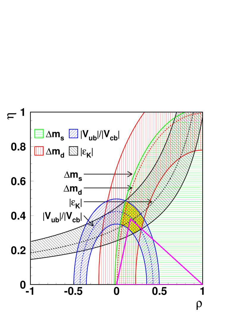
Figure 2: The current constraints and the favoured unitarity triangle. The constraint coming from $\mathrm{B}^{0}_{\mathrm{s}}$ oscillations is a limit at 95% of Confidence Level, while the others represent a $\pm 1\sigma$ variation of the experimental and theoretical parameters entering the formulae in the text.

This constraint gives a circle in the $\rho-\eta$ plane with centre in (0,0), shown in Figure 2 together with all the other constraints described above.

Determination of $\boldmath{\rho}$ and $\boldmath{\eta}$

The $\rho$ and $\eta$ parameters can be determined from a fit to the experimental values of all the constraints described above. The experimental and theoretical quantities that appear in the formulae describing the constraints have been fixed to their central values if their errors were reasonably small, and are reported in the left half of Table 1. The quantities affected by a larger error have been used as additional parameters of the fit, but including a constraint on their value. This procedure has been implemented making use of the MINUIT package [22] to minimise the following expression:

$$\chi^{2}={\left(\widehat{A}-A\right)^{2}\over\sigma_{A}^{2}}+{\left(\widehat{m_{c}}-m_{c}\right)^{2}\over\sigma_{m_{c}}^{2}}+{\left(\widehat{m_{t}}-m_{t}\right)^{2}\over\sigma_{m_{t}}^{2}}+{\left(\widehat{B_{K}}-B_{K}\right)^{2}\over\sigma_{B_{K}}^{2}}+$$

$$+{\left(\widehat{\eta_{cc}}-\eta_{cc}\right)^{2}\over\sigma_{\eta_{cc}}^{2}}+{\left(\widehat{\eta_{ct}}-\eta_{ct}\right)^{2}\over\sigma_{\eta_{ct}}^{2}}+{\left(\widehat{f_{B_{d}}\sqrt{B_{B_{d}}}}-f_{B_{d}}\sqrt{B_{B_{d}}}\right)^{2}\over\sigma_{f_{B_{d}}\sqrt{B_{B_{d}}}}^{2}}+{\left(\widehat{\xi}-\xi\right)^{2}\over\sigma_{\xi}^{2}}+{\left(\widehat{|\mathrm{V_{ub}}|\over|\mathrm{V_{cb}}|}-{|\mathrm{V_{ub}}|\over|\mathrm{V_{cb}}|}\right)^{2}\over\ \sigma_{{|\mathrm{V_{ub}}|\over|\mathrm{V_{cb}}|}}^{2}}+$$

$$+{\left(\widehat{|\epsilon_{K}|}-|\epsilon_{K}|\right)^{2}\over\sigma_{|\epsilon_{K}|}^{2}}+{\left(\widehat{\Delta m_{d}}-\Delta m_{d}\right)^{2}\over\sigma_{\Delta m_{d}}^{2}}+\chi^{2}\left({\cal{A}}\left(\Delta m_{s}\right),\sigma_{\cal{A}}\left(\Delta m_{s}\right)\right).$$

The symbols with a hat represent the reference values measured or calculated for a given physical quantity, as listed in Table 1, while the corresponding $\sigma$ are their errors. The parameters of the fit are $\rho$, $\eta$, $A$, $m_{c}$, $m_{t}$, $B_{K}$, $\eta_{ct}$, $\eta_{cc}$, $f_{B_{d}}\sqrt{B_{B_{d}}}$ and $\xi$, that are used to calculate the values of $|\epsilon_{K}|$, $\Delta m_{d}$, $\Delta m_{s}$ and $|\mathrm{V_{ub}}|\over|\mathrm{V_{cb}}|$ by means of the formulae (2), (4), (5) and (6).

As no measurements of $\Delta m_{s}$ are available a further contribution to the $\chi^{2}$ analogous to the previous ones can not be calculated. The following approximation has been used to extract a contribution from the Confidence Levels of the $\Delta m_{s}$ exclusion. The results of the search for $B^{0}_{s}$ oscillations have been presented and combined [13] in terms of the oscillation amplitude ${\cal{A}}$ [23], a parameter that is zero in the absence of signal and compatible with one if an oscillation signal is observed, as in:

$$P\left[B^{0}_{s}\rightarrow(B^{0}_{s},\bar{B^{0}_{s}})\right]={1\over 2\tau_{s}}e^{-t/\tau_{s}}\left(1\pm{\cal{A}}\cos{\Delta m_{s}}\right).$$

The experimental results are reported in terms of ${\cal{A}}\left(\Delta m_{s}\right)$ and $\sigma_{\cal{A}}\left(\Delta m_{s}\right)$, which leads to the quoted 95% Confidence Level limit as the value of $\Delta m_{s}$ for which the area above one of the Gaussian distribution with mean ${\cal{A}}\left(\Delta m_{s}\right)$ and variance $\sigma^{2}_{\cal{A}}\left(\Delta m_{s}\right)$ equals the 5% of the total area. As noted in [24] the full set of combined ${\cal{A}}\left(\Delta m_{s}\right)$ and $\sigma_{\cal{A}}\left(\Delta m_{s}\right)$ measurements indeed contains more information than this limit and it is used in this procedure, with a different statistical approach. The value of $\Delta m_{s}$ can be calculated for each value taken by the fit parameters $\rho$, $\eta$ and $\xi$ by means of formula (5), together with the value of its corresponding Confidence Level obtained as described above. The value $\chi^{2}\left({\cal{A}}\left(\Delta m_{s}\right),\sigma_{\cal{A}}\left(\Delta m_{s}\right)\right)$ of a $\chi^{2}$ distribution with one degree of freedom corresponding to this Confidence Level can then be calculated and added to the total $\chi^{2}$ of the fit.

		Fixed in the fit			Varied in the fit
$\lambda$	=	$0.2196\pm 0.0023$	$A$	=	$0.819\pm 0.035$
$G_{F}$	=	$(1.16639\pm 0.00001)\times 10^{-5}$ GeV-2	$\eta_{ct}$	=	$0.47\pm 0.04$
$f_{K}$	=	$0.1598\pm 0.0015$ GeV	$\eta_{cc}$	=	$1.38\pm 0.53$
$\Delta m_{K}$	=	$(0.5304\pm 0.0014)\times 10^{-2}$ ps-1	$\overline{m_{c}}(m_{c})$	=	$1.25\pm 0.15$ GeV
$m_{K}$	=	$0.497672\pm 0.000031$ GeV	$\overline{m_{t}}(m_{t})$	=	$166.8\pm 5.3$ GeV
$m_{W}$	=	$80.375\pm 0.064$ GeV	$f_{B_{d}}\sqrt{B_{B_{d}}}$	=	$0.201\pm 0.042$ GeV
$m_{B_{d}}$	=	$5.2792\pm 0.0018$ GeV	$B_{K}$	=	$0.87\pm 0.14$
$m_{B_{s}}$	=	$5.3692\pm 0.0020$ GeV	$\xi$	=	$1.14\pm 0.08$
$m_{B}$	=	$5.290\pm 0.002$ GeV	$|\epsilon_{K}|$	=	$(2.280\pm 0.019)\times 10^{-3}$
$\eta_{B}$	=	$0.55\pm 0.01$	$\Delta m_{d}$	=	$0.471\pm 0.016$ ps-1
$\eta_{tt}$	=	$0.574\pm 0.004$	$|\mathrm{V_{ub}}|/|\mathrm{V_{cb}}|$	=	$0.093\pm 0.016$

Table 1: Physical constants and parameters of the fit. The values whose origin is not discussed in the text are from [5].

The results of the fit are the following:

$$\rho=0.160^{+0.094}_{-0.070}\,\,\,\,\,\eta=0.381^{+0.061}_{-0.058}.$$

The 95% Confidence Level regions for $\rho$ and $\eta$ are:

$$-0.02<\rho<0.35\,\,\,\,\,0.27<\eta<0.50\,\,\,(\mathrm{95\%C.L.}).$$

Figure 3a shows the allowed confidence regions in the $\rho-\eta$ plane, together with the favoured unitarity triangle, that is also shown superimposed on the constraints of Figure 2.

From these results it is possible to determine also the value of the angles of the unitarity triangle. The angles $\alpha$ and $\beta$ are reported in terms of the functions $\sin{2\alpha}$ and $\sin{2\beta}$ as will be measured at the next B-factories. The numerical values obtained from the fit are:

$$\sin{2\alpha}=0.06^{+0.35}_{-0.42}\,\,\,\,\,\sin{2\beta}=0.75\pm 0.09\,\,\,\,\,\gamma=67^{+11}_{-12}\,{}^{\circ}.$$

In terms of 95% Confidence Level regions these last results can be expressed as:

$$-0.71<\sin{2\alpha}<0.70\,\,\,\,\,0.56<\sin{2\beta}<0.94\,\,\,\,\,44^{\circ}<\gamma<93^{\circ}\,\,\,(\mathrm{95\%C.L.})$$

Interpretations

The fit procedure described above can also be used to extract information on the theory parameters that enter the fit with a large uncertainty and at the same time, perform an estimation of $\rho$ and $\eta$ independent of them. This can be achieved by removing from the fit the constraint on the parameter. The two parameters $B_{K}$ and $f_{B_{d}}\sqrt{B_{B_{d}}}$ are those affected by the largest theory uncertainty. By applying this method to the parameter $B_{K}$, the fit yields:

$$\rho=0.156^{+0.096}_{-0.091}\,\,\,\,\,\eta=0.393^{+0.072}_{-0.080}\,\,\,\,\,B_{K}=0.80^{+0.27}_{-0.16}.$$

The value of $B_{K}$ favoured by the fit has an error larger than that on the estimated input parameter and thus can not help in restricting its range of allowed values. The same procedure with $f_{B_{d}}\sqrt{B_{B_{d}}}$ as a free parameter leads to the results:

$$\rho=0.186^{+0.085}_{-0.093}\,\,\,\,\,\eta=0.379^{+0.061}_{-0.057}\,\,\,\,\,f_{B_{d}}\sqrt{B_{B_{d}}}=0.222^{+0.026}_{-0.011}\,{\mathrm{\ Ge\kern-1.00006ptV}},$$

the value of $f_{B_{d}}\sqrt{B_{B_{d}}}$ comes out to be well in agreement with the predicted one with a smaller uncertainty. The same procedure applied to $B_{K}$ and $f_{B_{d}}\sqrt{B_{B_{d}}}$ simultaneously gives:

$$\rho=0.170^{+0.320}_{-0.098}\,\,\,\,\,\eta=0.390^{-0.059}_{-0.103}\,\,\,\,\,B_{K}=0.82^{+0.41}_{-0.17}\,\,\,\,\,f_{B_{d}}\sqrt{B_{B_{d}}}=0.217^{+0.047}_{-0.022}\,{\mathrm{\ Ge\kern-1.00006ptV}}.$$

The $\Delta m_{s}$ constraint has a big impact on the $\rho$ uncertainty as can be observed by removing it from the fit, what gives:

$$\rho=0.022_{-0.264}^{+0.145}\,\,\,\,\,\eta=0.434_{-0.090}^{+0.062}.$$

Figure 3b shows the experimentally favoured regions in the $\rho-\eta$ plane for this fit together with the lower limit and expected sensitivity ($\Delta m_{s}=13.8\,\mathrm{ps}^{-1}$ [15]) of the current experiments to $B^{0}_{s}$ oscillations. The confidence regions for $\Delta m_{s}$ can be extracted from this fit as:

$$\Delta m_{s}=11.3_{-3.9}^{+3.0}\,\mathrm{ps}^{-1}\\$$

$$5.7\,\mathrm{ps}^{-1}<\Delta m_{s}<17.8\,\mathrm{ps}^{-1}\,\,\,(\mathrm{95\%C.L.}),$$

The LEP measurements have greatly improved the constraints on the CKM matrix. Another fit has been performed removing the $\Delta m_{s}$ constraint, derived mainly from the LEP limits, and excluding the LEP measurement from the averages of the other input quantities; that is using:

$$|\mathrm{V_{ub}}|/|\mathrm{V_{cb}}| = 0.08\pm 0.02$$

$$|\mathrm{V_{cb}}| = (50\pm 5)\times 10^{-3}$$

$$\Delta m_{d} = (0.500\pm 0.030)\,\mathrm{ps}^{-1}.$$

The first value is that quoted above from the CLEO collaboration [16], the second follows from [25] and the last has been estimated from the current published and preliminary results from the CDF and SLD collaborations. This fit, as shown in Figure 3c, yields:

$$\rho=0.012^{+0.192}_{-0.252}\,\,\,\,\,\eta=0.383^{+0.082}_{-0.093}\,\,\,\mathrm{and}$$

$$\sin{2\alpha}=0.63^{+0.37}_{-0.90}\,\,\,\,\,\sin{2\beta}=0.67^{+0.14}_{-0.22}\,\,\,\,\,\gamma=88^{+39}_{-28}\,{}^{\circ}.$$

Some of the errors are reduced by as much as a factor three by the inclusion of the LEP data.

A real CKM matrix ?

To date the only experimental evidence for the violation of CP in the CKM matrix, namely its complex phase described by a value of $\eta$ different from zero, comes from the neutral kaon system. As different models have been proposed to explain that effect, it is of interest to remove from the fit the constraint related to this process and then investigate the compatibility of $\eta$ with zero [26]. This procedure yields the following results, graphically displayed in Figure 3d:

$$\rho=0.156_{-0.090}^{+0.096}\,\,\,\,\,\eta=0.394_{-0.080}^{+0.072}.$$

The value of $\eta$ is not compatible with zero at the 95% and 99% of Confidence Levels either:

$$-0.025<\rho<0.358\,\,\,(\mathrm{95\%C.L.}) \,\,\,\,\,\,-0.069<\rho<0.411\,\,\,(\mathrm{99\%C.L.})$$

$$0.224<\eta<0.531\,\,\,(\mathrm{95\%C.L.}) \,\,\,\,\,\,\phantom{-}0.157<\eta<0.574\,\,\,(\mathrm{99\%C.L.}).$$

If the CKM matrix is assumed to be real, as recently proposed for instance in [27], all the circular constraints reduce to linear intervals on the $\rho$ axis, onto which the unitarity triangle will then be projected. This hypothesis can be checked removing again the neutral kaon constraints from the fit and modifying the formulae (4), (5) and (6) imposing $\eta$ equal to zero. The result of this fit, whose parameters are reduced to $\rho$, $A$, $m_{t}$, $f_{B_{d}}\sqrt{B_{B_{d}}}$ and $\xi$, is:

$$\rho=0.321_{-0.056}^{+0.053}.$$

The value of the $\chi^{2}$ function at the minimum is 6.7, leading to the conclusion that a CKM matrix real by construction can fit the data.

Conclusions

The combination of the precise measurements of $\Delta m_{d}$, the updated limits on $\Delta m_{s}$ and the determination of $|\mathrm{V_{ub}}|$ helps in constraining the CKM matrix elements.

From a simultaneous fit to all the available data and theory parameters the vertex of the unitarity triangle is determined as:

$$\rho=0.160^{+0.094}_{-0.070}\,\,\,\,\,\eta=0.381^{+0.061}_{-0.058}.$$

yielding the following values for its angles:

$$\sin{2\alpha}=0.06^{+0.35}_{-0.42}\,\,\,\,\,\sin{2\beta}=0.75\pm 0.09\,\,\,\,\,\gamma=67^{+11}_{-12}\,{}^{\circ}.$$

The accuracy on $\sin{2\beta}$ from this indirect analysis is already at the same level as that expected to be achieved with the direct measurement at the B-factories due to become operational in the next future. These limits greatly benefit from the inclusion of LEP data.

The fit suggests the value of the non-perturbative QCD parameter $f_{B_{d}}\sqrt{B_{B_{d}}}$ as:

$$f_{B_{d}}\sqrt{B_{B_{d}}}=0.222^{+0.026}_{-0.011}\,{\mathrm{\ Ge\kern-1.00006ptV}}.$$

The parameter $\eta$ related to the complex phase of the matrix and thus to the CP violation is found to be different from zero at more than the 99% Confidence Level, even removing from the fit the constraints arising from CP violation in the neutral kaon system. Nonetheless the hypothesis of a real matrix can still fit the data without this constraint.

The fit also indicates the $\Delta m_{s}$ variation range as:

$$\Delta m_{s}=(11.3_{-3.9}^{+3.0})\,\mathrm{ps}^{-1}$$

$$5.7\,\mathrm{ps}^{-1}<\Delta m_{s}<17.8\,\mathrm{ps}^{-1}\,\,\,(\mathrm{95\%C.L.}).$$

These results improve those of similar previous analyses  [24, 28] and agree with another one based on a different approach [15].

Figure 1: The unitarity triangle.

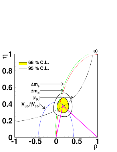
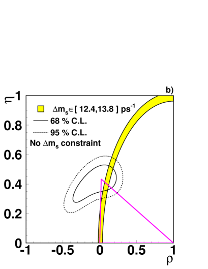
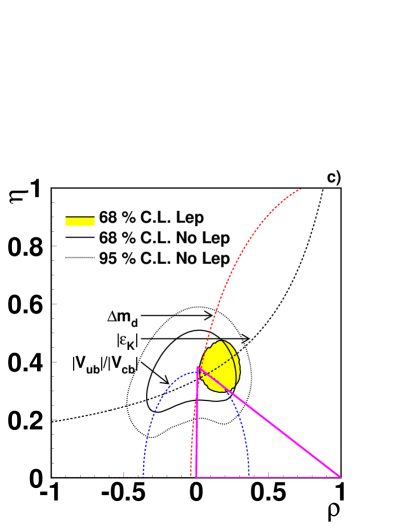
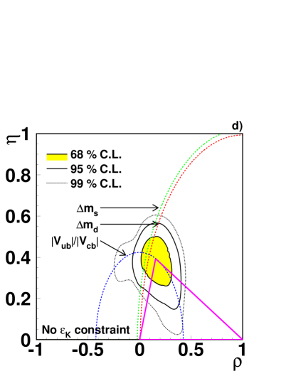
Figure 3: The favoured unitarity triangles and the confidence regions for their vertices in the following assumptions: a) the fit using all data described in the text, b) the constraint from the $\mathrm{B}^{0}_{\mathrm{s}}$ oscillations is not applied, c) the LEP measurements are excluded from the fit, d) no constraints from the neutral kaon system are applied. The band in b) displays the values of $\rho$ and $\eta$ corresponding to a value of $\Delta m_{s}$ between the current lower limit and expected sensitivity. The $\Delta m_{s}$ limit and the central values of the constraints are shown in a), c) and d).

References

• [1] S. L. Glashow, Nucl. Phys. 22 (1961) 579; A. Salam, in Proceedings of the VIIIth Nobel Symposium, ed. N. Svartholm, (Almquist and Wiksell, Stockholm, 1968), p. 367; S. Weinberg, Phys. Rev. Lett. 19 (1967) 1264.
• [2] N. Cabibbo, Phys. Rev. Lett. 10 (1963) 531; M. Kobayashi and K. Maskawa, Prog. Theo. Phys. 49 (1973) 652.
• [3] L. Wolfenstein, Phys. Rev. Lett. 51 (1983) 1945.
• [4] A. Ali and D. London, Z. Phys. C 65 (1995) 431.
• [5] Particle Data Group, Eur. Phys. J. C 3 (1998) 1.
• [6] T. T. Wu and C. N. Yang, Phys. Rev. Lett. 13 (1964) 380.
• [7] A. J. Buras et al., Nucl. Phys. B 238 (1984) 529.
• [8] A. J. Buras et al., Nucl. Phys. B 245 (1984) 369.
• [9] A. J. Buras et al., Nucl. Phys. B 347 (1990) 491.
• [10] A. J. Buras, Nucl. Inst. Meth. A 368 (1995) 1; A. Buchalla et al., Nucl. Phys. B 337 (1990) 313; W. A. Kaufman et al., Mod. Phys. Lett. A 3 (1989) 1479; J. M. Flynn et al., Mod. Phys. Lett. A 5 (1990) 877; A. Datta et al., Z. Phys. C 46 (1990) 63; S. Herrlich et al., Nucl. Phys. B 419 (1994) 292.
• [11] JLQCD Collab., S. Aoki et al., Nucl. Phys. B (Proc. Suppl) 63A-C (1998) 281.
• [12] S. R. Sharpe, Nucl. Phys. B (Proc. Suppl) 53 (1997) 181.
• [13] J. Alexander, XXIXth International Conference on High Energy Physics, Vancouver 1998, to appear in the Proceedings.
• [14] J. M. Flynn and C. T. Sachrajda, hep-lat/9710057, to appear in Heavy Flavours (2nd edition) ed. by A. J. Buras and M. Linder (World Scientific, Singapore).
• [15] F. Parodi, XXIXth International Conference on High Energy Physics, Vancouver 1998, to appear in the Proceedings.
• [16] CLEO Collab., J. Bartelt et al., Phys. Rev. Lett. 71 (1993) 4111.
• [17] N. G. Uraltsev, Int. Jour. of Mod. Phys. A 11 (1996) 515; I. Bigi et al., Ann. Rev. Nucl. Part. Sci. 47 (1997) 591.
• [18] ALEPH Collab., R. Barate et al., Preprint CERN-EP/98-067, 1998.
• [19] L3 Collab., M. Acciarri et al., Preprint CERN-EP/98-097, 1998.
• [20] R. Bately, XXXIIIrd Rencontres de Moriond, Electroweak Interactions and Unified Theories, 1998, to appear in the Proceedings.
• [21] DELPHI Collab., M. Battaglia et al., DELPHI note 98-97, 1998.
• [22] F. James, MINUIT Reference Manual, CERN Program Library Long Writeup D506, 1994.
• [23] H. G. Moser and A. Roussarie, Nucl. Inst. Meth. A 384 (1997) 491.
• [24] F. Paganini et al., Preprint LAL-97-79, 1997.
• [25] J. R. Patterson, in Proceedings of the XXVIIth International Conference on High Energy Physics, Glasgow, 1994, ed. I. G. Knowles P. J. Bussey, (Institute of Physics Publishing, Bristol and Philadelphia, 1994), p. 149.
• [26] R. Barbieri et al., Phys. Lett. B 425 (1998) 119.
• [27] H. Georgi and S. L. Glashow, Preprint HUTP-98/A048, 1998.
• [28] A. Ali and B. Kayser, hep-ph/9806320, to appear in The Particle Century ed. by G. Fraser (Institute of Physics Publishing, Bristol and Philadelphia); Y. Grossman et al., Nucl. Phys. B 511 (1998) 69; F. Parodi et al., Preprint LAL-98-49, 1998; S. Mele, hep-ph/9808411, Workshop on CP Violation, Adelaide 1998, to appear in the Proceedings.
Refer to caption