Historical and other Remarks on Hidden Symmetries
(Norbert Straumann, University of Zürich)

Apart from a few remarks on lattice systems with global or gauge symmetries, most of this talk is devoted to some interesting ancient examples of symmetries and their breakdowns in elasticity theory and hydrodynamics. Since Galois Theory is in many ways the origin of group theory as a tool to analyse (hidden) symmetries, a brief review of this profound mathematical theory is also given.

Introductory Remarks

The organisers have asked me to entertain you in an evening lecture with some historical episodes, related to symmetries and their spontaneous breakdowns, the main theme of this Summer School. This is indeed a fascinating subject. I shall begin with ancient examples, connected with great names, like Euler, Galois, Jacobi, $\cdot\cdot\cdot$. In a second part of my talk I would, however, like to add a few non-historical remarks which are relevant for (lattice) field theory. These should be regarded as supplements to the lectures by Lochlainn O’Raifeartaigh, Daniel Loss, and others.

In one hour I cannot cover the various topics in any depth. To compensate for this, I shall add a few references to sources which I find interesting and pleasant to read.

Contents

1. 1 Euler’s instability analysis of rods under longitudinal compressional forces
2. 2 Galois Theory, the origin of group theory to analyse symmetries
   1. 2.1 Basic concepts and fundamental theorem of Galois Theory
   2. 2.2 Solutions by radicals
   3. 2.3 Ruler and compass constructions
3. 3 Rotating selfgravitating equilibrium figures
4. 4 Spontaneous symmetry breaking due to thermal instabilities
5. 5 Goldstone- and Mermin-Wagner theorems
   1. 5.1 Spontaneous symmetry breaking for the Ising model (d$\geq$2)
   2. 5.2 Spin systems with continuous symmetry groups
6. 6 Order parameters and Elitzur’s theorem for gauge theories

1 Euler’s instability analysis of rods under longitudinal compressional forces

Leonhard Euler, the man who created more mathematics than anybody else in history, was also one of the leading figures in the development of elasticity theory [1]. In one of his later works on this subject, ”Determinatio onerum, quae columnae gestare valent” (Determination of loads which may be supported by columns), submitted to the Academy in Petersburg in 1776, Euler studies again the following problem.

Consider a thin (metal) rod of length $L$ and circular cross section of radius $R$. Assume that the rod is clamped at both ends and subjected to a compressional force $F$ directed along the rod axis ($z$ axis). We denote the deflections of the rod in the transversal $x$ and $y$ directions as functions of $z$ by $X(z)$ and $Y(z)$, respectively. For small deflections Euler derives from the theory of elasticity the following differential equations

$$IE~{}\frac{d^{4}X}{dz^{4}}+F~{}\frac{d^{2}X}{dz^{2}} = 0~{},$$

$$IE~{}\frac{d^{4}Y}{dz^{4}}+F~{}\frac{d^{2}Y}{dz^{2}} = 0~{},$$ (1.1)

where $E$ is the Young’s modulus (which was actually introduced already by Euler in the paper mentioned above) and $I$ is the moment of inertia, $I=1/4~{}\pi R^{4}$. (For a textbook derivation of these equations, see [2].)

The boundary conditions of the clamped rod are

$$X(0)=X(L)=0~{},$$

$$\frac{dX}{dz}(0)=\frac{dX}{dz}(L)=0~{},$$ (1.2)

and similarly for $Y$.

Clearly, as long as the force $F$ is sufficiently small, the rod will be straight; that is, the only solution of (1.1) and (1.2) will be $X(z)=Y(z)\equiv 0$, and the rod is stable. However, if $F$ is increased there will be a critical value $F_{c}$, above which the rod is unstable against small perturbations from straightness and will bend (see Fig.1).

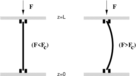
Figure 1: Elastic instability of a longitudinally compressed rod.

Although in general the deflection will be large, equations (1.1) can still be used to find the critical value $F_{c}$. We just have to find out when (1.1) will have a nontrivial solution $X(z)$, satisfying the boundary conditions (1.2).

The most general solution of (1.1) for $X(z)$ is

$$X(z)=A+Bz+C\sin(kz)+D\cos(kz)~{},~{}~{}k=\sqrt{\frac{F}{EI}}~{}.$$ (1.3)

The boundary conditions (1.2) imply two branches of solutions. One is given by

$$X={\rm const}~{}(1-\cos(kz))~{},~{}~{}kL=2\pi n~{}~{}(n=1,2,...)~{},$$ (1.4)

and for the other $k$ has to satisfy $\tan(kL/2)=kL/2$.
The critical value $F_{c}$ corresponds to the lowest mode with $n=1$ (no node), whence

$$F_{c}=\frac{4\pi^{2}EI}{L^{2}}~{}~{}(\rm{Euler})~{}.$$ (1.5)

For $n=1$ the deflection (1.4) can be written as

$$X(z)={\rm const}\sin^{2}\left(\frac{\pi z}{L}\right)~{}.$$ (1.6)

When $F$ becomes larger than $F_{c}$, the system, when perturbed infinitesimally, jumps to a new ground state in which the U(1) symmetry is broken (the bent rod). This new state is degenerate, since the rod can be bent in any plane containing the $z$ axis. This is a nice example of the phenomenon of spontaneous symmetry breaking (SSB).

The relevance of the criterion (1.5) for engineering is obvious. Euler has also studied the shapes of bent rods undergoing large deflections. (This is discussed in [2], §19.)

2 Galois Theory, the origin of group theory to analyse symmetries

I come now to an entirely different chapter.

One of the main contributions of Galois was to identify the group concept and to use it to analyse the problem of solvability of polynomial equations by radicals. This enabled him to find a criterion of solvability which has unsolvability of the general quintic as just one of many corollaries. Galois theory is in many ways the origin of group theory as a tool to analyse symmetries. It may thus not be completely out of place to make a few remarks about this very beautiful and profound theory, even if it has, so far, no direct applications in physics. (The relations between physics and pure mathematics are much more subtle than most physicists are aware of.) Galois Theory nowadays plays an important role in algebraic geometry and number theory.

2.1 Basic concepts and fundamental theorem of Galois Theory

In Galois Theory one studies field extensions $K$ of a base field $F$. The extension $K$ of $F$ ($F\subset K$) may be regarded as a vector space over $F$. We write [$K:F$] for the dimension of $K$ as an $F$-vector space and assume always that this is finite. The pair $F\subset K$ is then called a finite extension. The reader may assume (for simplicity) that all fields are subfields of the complex numbers $\mathbb{C}$ containing the rational numbers $\mathbb{Q}$. A simple example is $\mathbb{R}\subset\mathbb{C}$, with $[\mathbb{C}:\mathbb{R}]=2$.

Important examples of field extensions arise as follows. Consider a polynomial $p(X)$ in the indeterminate $X$,

$$p(X)=a_{0}+a_{1}X+...+a_{n}X^{n},$$ (2.1)

whose coefficient are (for instance) in $\mathbb{Q}$. Let $\alpha_{1},...,\alpha_{n}$ be the roots of $p(X)$ in $\mathbb{C}$. The smallest subfield of $\mathbb{C}$, containing $\mathbb{Q}$ as well as the roots $\alpha_{1},...,\alpha_{n}$, is denoted by $\mathbb{Q}(\alpha_{1},...,\alpha_{n})$ and is called the splitting field of $p$ over $\mathbb{Q}$. (This notion can, of course, be generalised to arbitrary fields $F$ and polynomials over $F$, instead of $\mathbb{Q}$.)

For finite extensions $F\subset K$ the field $K$ is algebraic over $F$, i.e., for every $\alpha\in K$ there is a polynomial $f\in F[X]$, such that $f(\alpha)=0$.

The Galois group, $Gal(K/F)$, of a field extension $F\subset K$ consists of all automorphisms of $K$ which leave the elements of $F$ fixed. For finite extensions the Galois group is always finite. Clearly, the fixed set $Fix(Gal(K/F))$, consisting of all elements of $K$ which are left invariant under $Gal(K/F)$, contains $F$, but may in general be larger. We say that $F\subset K$ is a Galois extension, if

$$Fix(Gal(K/F))=F~{}.$$ (2.2)

One can show that this is equivalent to

$$|Gal(K/F)|=[K:F]~{}.$$ (2.3)

(For a finite group $G$, the number of elements is denoted by $|G|$.) This is just one of several characterizations of Galois extensions.

Now we come to a first central result, which provides a key to analyse the structure of field extensions with the help of group theory.

Theorem 1 (Fundamental Theorem of Galois Theory.)

Let $K$ be a finite Galois extension of $F$, and let $G=Gal(K/F)$. Then there is a 1-1 inclusion reversing correspondence between intermediate fields $L~{}(F\subset L\subset K)$ and subgroups of $G$, given by

$$L\longmapsto Gal(K/L)$$ (2.4)

and

$$H\longmapsto Fix(H)~{}~{}(H\subset G)~{}.$$ (2.5)

Furthermore, if $L\longleftrightarrow H$, then $[K:L]=|H|$ and $[L:F]=[G:H]$ (= order of $G$ in $H$). Moreover, $H$ is a normal subgroup of $G$ if and only if $L$ is Galois over $F$. When this occurs,

$$Gal(L/F)\cong G/H~{}.$$ (2.6)

2.2 Solutions by radicals

Consider the polynomial equation $p(X)=0$, with a polynomial $p(X)$ of the form (2.1). The elements obtained from $a_{0},...,a_{n}$ by the operations $+,\cdot,\div$ form the coefficient field $\mathbb{Q}(a_{0},...,a_{n})$. An element obtained from this field by a finite number of roots $~{}\sqrt[]{~{}~{}},\sqrt[3]{~{}~{}},\sqrt[4]{~{}~{}},...$ lies in an extension field of $\mathbb{Q}(a_{0},...,a_{n})$ obtained by a finite number of radical adjunctions. We say that adjunctions of an element $\alpha$ to a field $F$ is radical if there is a positive integer $m$ such that $\alpha^{m}\in F$. The result of several radical adjunctions $F(\alpha_{1})...(\alpha_{k})$ is called a radical extension of $F$ and is denoted by $F(\alpha_{1},...,\alpha_{k})$.

Thus the problem of solution by radicals is to find a radical extension of the coefficient field $\mathbb{Q}(\alpha_{0},...,\alpha_{n})$ which includes the roots $x_{1},...,x_{n}$ of

$$a_{0}+a_{1}x+...+a_{n}x^{n}=0.$$ (2.7)

For example, the formula for the solution of the quadratic equation with $a_{2}=1$,

$$x_{1,2}=\frac{-a_{1}\pm\sqrt{a_{1}^{2}-4a_{0}}}{2}~{},$$

shows that $\mathbb{Q}(x_{1},x_{2})$ is contained in the radical extension $\mathbb{Q}(a_{0},a_{1},\sqrt{a_{1}^{2}-4a_{0}})$.

A classical application of Galois Theory, and one of the main results of Galois himself, is the following

Theorem 2 (Galois)

A polynomial $f\in\mathbb{Q}[X]$ with splitting field $K$ over $\mathbb{Q}$ is solvable by radicals if and only if the Galois group $Gal(K/\mathbb{Q})$ is solvable. (Here, $\mathbb{Q}$ can be replaced by any field of characteristic 0.)

We recall that a group $G$ is solvable if there is a chain of subgroups

$$<e>=H_{0}\subseteq H_{1}\subseteq...\subseteq H_{n}=G~{},$$

such that for all $i$, the subgroup $H_{i}$ is normal in $H_{i+1}$ and the quotient group $H_{i+1}/H_{i}$ is Abelian.

Consider, for instance, the equation

$$x^{5}-4x+2=0~{}.$$ (2.8)

It is not difficult to show that the Galois group of this equation (i.e., the Galois group $Gal(K/\mathbb{Q})$, $K$ being the splitting field of $f(X)=X^{5}-4X+2$) is the permutation group $S_{5}$, which is not solvable. (The latter fact can be proven in a very elementary way.) Galois’ theorem thus implies that (2.8) is not solvable by radicals.

2.3 Ruler and compass constructions

Galois Theory can also be used to answer some ancient questions concerning constructions with ruler and compass. Examples are:

• Is it possible to trisect any angle?

• Is it possible to double the cube?

• For which $n$ is it possible to construct a regular $n$-gon?

Let me only address the third question, whose solution makes use of much of Galois Theory. Consider first the case when $n$ is a prime number $p$. In this case we have the

Theorem 3

A regular $p$-gon ($p$ a prime number) is constructible if and only if $p-1$ is a power of 2.

Such numbers are called Fermat primes. Unfortunately, we do not know whether there are any Fermat primes beyond

$$3,5,17,257,65537~{}.$$ (2.9)

Deciding whether 65537 is the last Fermat prime may well tax the best mathematician of the future. Fermat had conjectured (1640) that $2^{2^{h}}+1$ is prime for all natural numbers $h$, but Euler found (1738) that 641 divides $2^{2^{5}}+1$.

The theorem above implies, for example, that a regular 17-gon is constructible. An explicit construction was given by the 19-year old Gauss in 1796.

For the general case we have to introduce the Euler phi function $\phi(n)$. This counts those integers among $1,2,...,n-1$ which have no nontrivial common divisors with $n$. (For a prime, we clearly have $\phi(p)=p-1$.) The last theorem generalizes to:

Theorem 4

A regular $n$-gon is constructible if and only if $\phi(n)$ is a power of 2.

If $n=p_{1}^{m_{1}}...p_{r}^{m_{r}}$ is the prime factorization of $n$, then $\phi(n)=\prod_{i}p^{m_{i}-1}(p_{i}-1)$. It is not difficult to show that $\phi(n)$ is a power of 2 if and only if

$$n=2^{s}q_{1}...q_{r}~{},$$ (2.10)

where the $q_{i}$ are Fermat primes. In this sense problem (iii) is solved. But remember, we may not know all Fermat primes.

Discussion

Galois’ work was to sketchy to be understood by his referees, and it was not published in his brief lifetime (he died after a duel in 1832, aged 20). It was later published by Liouville in 1846, after he became convinced that Galois’ proof of his solvability criterion of equations was correct. Over the next two decades the group concept was then assimilated to the point where Jordan could write his ”Trait$\acute{{\rm e}}$ des substitutions et des $\acute{{\rm e}}$quations alg$\acute{{\rm e}}$brique” in 1870. This book is inspired by Galois Theory, but group theory takes over almost completely.

In the 1870s geometry also began to influence group theory. Of great importance was Klein’s Erlanger Programm in 1872, which emphasized the unifying role of groups in geometry. In those days nobody could imagine that group theory would one day play also in physics such a decisive and increasingly important role.

Among the many excellent textbooks on Galois Theory, I refer to the recent one by J. Stillwell [3], which is written in a lively style, emphasizing the historical context, and avoiding unnecessary generalizations (for beginners).

3 Rotating selfgravitating equilibrium figures

For nearly a century it was believed that Maclaurin’s axially symmetric ellipsoids (1742) represent the only admissable solutions of the problem of the equilibrium of selfgravitating uniformly rotating homogeneous masses.

In 1834 Jacobi came up with the surprising announcement:

”One would make a grave mistake if one supposed that the spheroids of revolution are the only admissable figures of equilibrium even under the restrictive assumption of second degree surfaces. $\cdot\cdot\cdot$ In fact a simple consideration shows that ellipsoids with three unequal axes can very well be figures of equilibrium; and that one can assume an ellipse of arbitrary shape for the equatorial section and determine the third axes (which is also the least of the three axes) and the angular velocity of rotation such that the ellipsoid is a figure of equilibrium.”

Jacobi’s surprising discovery can be regarded as an example of spontaneous symmetry breaking of the group U(1). For small angular momenta there is only the symmetric solution, but above some bifurcation point there exists also an unsymmetric solution. Before saying more about this and the stability issue, let me enter a bit into the preceding history, which begins with Newton.

In the Principia, Book III, Propositions XVIII-XX, Newton derives the oblateness of the Earth and other planets. I first give his result.

Let

$$\epsilon=\frac{\rm{equatorial~{}radius-polar~{}radius}}{\rm{mean~{}radius~{}(R)}}$$ (3.1)

be the ellipticity, $M$ the total mass, $\Omega$ the angular velocity, and $R$ the average radius of the planet. With a beautiful argument (described below) Newton finds that

$$\epsilon=\frac{5}{4}\frac{\Omega^{2}R^{3}}{GM}~{},$$ (3.2)

if the body is assumed to be homogeneous.

In his derivation, Newton imagines a hole of unit cross-section drilled from a point of the equator to the center of the Earth and a similar hole from the pole to the center. Both ’canals’ are imagined to be filled with water (see Fig.2). Newton studies now the implication of the equilibrium condition:

$$\rm{weight~{}of~{}equilibrium~{}column=weight~{}of~{}polar~{}column}.$$ (3.3)

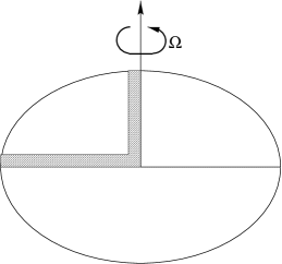
Figure 2: Newton’s water ’canals’ through the Earth.

Along the equator the acceleration due to gravity is ’diluted’ by the centrifugal acceleration. Newton has shown earlier (Book I, Propositions LXXIII and Corollary III, Proposition XCI) that both these accelerations, in a homogeneous body, vary from the center linearly with the distance. Therefore, the dilution factor remains constant and is equal to its value, $m$, on the boundary

$$m=\frac{\rm{centrifugal~{}acceleration~{}at~{}the~{}equator}}{\rm{mean~{}gravitational~{}acceleration~{}on~{}the~{}surface}}=\frac{\Omega^{2}R}{GM/R^{2}}~{}.$$ (3.4)

(Here, $m<<1$ is used.)

Now, the weight of the equatorial column is equal to $\frac{1}{2}\rho ag_{\rm{eq}}(1-m)$ ($a$=equatorial radius), and the weight of the polar column is $\frac{1}{2}\rho cg_{\rm{pole}}$ ($c$=polar radius). Thus eq.(3.3) gives

$$ag_{\rm{eq}}(1-m)=cg_{\rm{pole}}~{}.$$ (3.5)

Newton recognizes that this equation is valid for any $\epsilon$!
Using also $c=(1-\epsilon)a$ this gives

$$\frac{g_{\rm{pole}}}{g_{\rm{eq}}}=\frac{a}{c}(1-m)=\frac{1-m}{1-\epsilon}\simeq(1+\epsilon-m)~{}.$$ (3.6)

Chandrasekhar explains in his beautiful last book ([4], p. 386), how Newton arrived at the relations

$$g_{\rm{eq}}=\frac{4\pi}{3}a(1-\frac{2}{5}\epsilon),~{}~{}g_{\rm{pole}}=\frac{4\pi}{3}a(1-\frac{1}{5}\epsilon)~{}.$$ (3.7)

(For us it is easier to derive this from the Maclaurin solutions.)
If this is used in (3.6), Newton’s result

$$\epsilon=\frac{5}{4}m$$ (3.8)

is obtained.

It was known already in Newton’s time that for the Earth $m\simeq 1/290$. Therefore, Newton concludes that if the Earth were homogeneous, it should be oblate with an ellipticity

$$\epsilon\simeq\frac{5}{4}\frac{1}{290}\simeq\frac{1}{230}~{}.$$ (3.9)

We know that the actual ellipticity of the Earth is substantially smaller ($\simeq$1/294). This is interpreted in terms of the inhomogeneity of the Earth.

Newton’s prediction was against the ideas of the Cassini school, as is illustrated in the old-time caricature below (Fig.3).

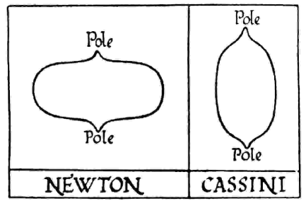
Figure 3: Caricature of the controversy on the figure of the Earth.

The famous controversy was finally settled by a measurement in 1738 of the arc of the meridian by a French expedition to Lapland, led by Maupertuis. This was an exceedingly difficult and tedious enterprise.

I. Todhunter writes in his ”A history of the mathematical theories of attraction and the figures of the Earth” in 1873 (reprinted by Dover Publications, p. 100):

”The success of the Arctic expedition may be fairly ascribed in great measure to the skill and energy of Maupertuis: and his fame was widely celebrated. The engravings of the period represent him in the costume of a Lapland Hercules, having a fur cap over his eyes; with one hand he holds a club, and with the other he compresses a terrestrial globe. Voltaire, then his friend, congratulated him warmly for having ’aplati les pôles et les Cassini’.”

Maupertuis’ report to the Paris Academy became a bestseller. A German translation appeared 1741 in Zürich.

I have to refrain to tell you more about Maupertuis, who later became the first President of the Prussian Academy, founded by Frederick the Great. Maupertuis was actually an organizer, but not a great scientist. His end was tragic.

After this long digression I come back to Jacobi’s solution. In Fig.4 the moment of inertia, $\Theta$, relative to the rotation axis (in units of the non-rotational case) is shown as a function of the angular velocity squared (in units of $\pi G\rho$, $\rho$=uniform density) for the Maclaurin and the triaxial Jacoby solutions. The latter sequence bifurcates from the axially symmetric family at the point where $\Omega^{2}/\pi G\rho=0.37423$ (eccentricity $\epsilon$=0.81267). One sees from Fig.4 that for $\Omega^{2}/\pi G\rho<0.37423$ there are three equilibrium figures possible: two Maclaurin spheroids and one Jacobi ellipsoid; for $0.4493>\Omega^{2}/\pi G\rho>0.3742$ only the Maclaurin figures are possible; and finally for $\Omega^{2}/\pi G\rho>0.4493$ there are no equilibrium solutions. (This enumeration was given by C.O. Meyer in 1842.)

As Riemann has shown, the Maclaurin ellipsoids become unstable in point $B$ in Fig.4, where $\Omega^{2}/\pi G\rho=0.4402$. Poincar$\acute{\rm{e}}$ and Cartan proved that the Jacobi sequence becomes unstable at $\Omega^{2}/\pi G\rho=0.2840$.

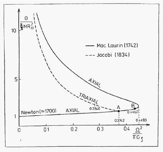
Figure 4: Maclaurin and Jacobi sequences of ellipsoidal equilibrium figures.

S. Chandrasekhar has devoted an entire book on the ellipsoidal figures of equilibrium and their stability analysis [5]. In Chapter 1 he gives a detailed discussion of the interesting history of this subject, to which an impressive list of great mathematicians, from Newton to Cartan, has contributed over a long period of time.

4 Spontaneous symmetry breaking due to thermal instabilities

Thermal instabilities often arise when a fluid is heated from below. A classical example is a horizontal layer of fluid with its lower side hotter than its upper. Due to thermal expansion, the fluid at the bottom will be lighter than at the top. When the temperature difference across the layer is great enough the stabilizing effects of viscosity and thermal conductivity are overcome by the destabilizing buoyancy, and an overturning instability ensues as thermal convection.

Such a convective instability seems to have been first described by James Thomson (1882), the elder brother of Lord Kelvin, but the first quantitative experiments were made by B$\acute{\rm{e}}$nard (1900). Stimulated by these experiments, Rayleigh formulated in 1916 the theory of convective instability of a layer of fluid between horizontal planes.

Starting from the basic hydrodynamic equations (in the Boussinesq approximation) and the boundary conditions, Rayleigh derived the linear equations for normal modes about the equilibrium solution. He then showed that an instability sets in when the following dimensionless parameter

$$R=g\alpha\beta d^{4}/\kappa\nu$$ (4.1)

exceeds a certain critical value $R_{c}$. Here $g$ is the acceleration due to gravity, $\alpha$ the coefficient of thermal expansion of the fluid, $\beta$ the magnitude of the vertical temperature gradient of the basic state at rest, $d$ the depth of the layer of the fluid, $\kappa$ the thermal conductivity and $\nu$ the kinematic viscosity. The parameter $R$ is now called the Rayleigh number.

If both boundaries are rigid, the critical value turns out to be

$$R_{c}=1707.762~{}.$$ (4.2)

(A detailed derivation can be found in [6], Chap.II. This beautiful book gives also the relevant references to the original literature.) Experimentally one found

$$R_{c}^{\rm{exp.}}=1700\pm 51~{},$$ (4.3)

in complete agreement with the theoretical value.

There is an ironic twist to what is cold B$\acute{\rm{e}}$nard convection. Most of the motions observed by B$\acute{\rm{e}}$nard, being in very thin layers with a free surface, were actually driven by variations of the surface tension with temperature and not by a thermal instability of a light fluid below a heavy one. This effect of the surface tension becomes, however, unimportant if the thickness of the layer is sufficiently large.

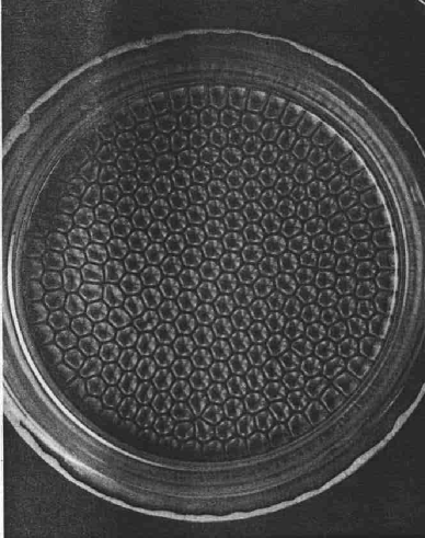
Figure 5: B$\acute{\rm{e}}$nard cells under an air surface.

When $R$ becomes larger then $R_{c}$, the motion of the fluid assumes a stationary, cellular character (spontaneous breakdown of translational symmetry). If the experiment is performed with sufficient care, the cells become equal and often form a regular hexagonal pattern (see Fig.5). As the Rayleigh number increases, a series of transitions from one complicated flow to the next more complicated one can be detected. An understanding of all this is difficult, because nonlinearities become significant.

This concludes my sundry of ancient examples on SSB.

5 Goldstone- and Mermin-Wagner theorems

Before Onsager had found his famous exact solution of the 2-dimensional Ising model, it was not generally accepted that the rules of statistical mechanics are able to describe phase transitions. As late as 1937, at the Van der Waals Centenary Conference, there was lively debate on whether phase transitions are consistent with the formalism of statistical mechanics. After the debate, Kramers suggested that a vote should be taken, on whether the infinite-volume limit could provide the answer. The result of that vote was close, but the infinite-volume limit did finally win. (More on this can be found in Pais’ wonderful biography of Einstein [7], pp. 432-33.)

We now know that first order phase-transitions in some parameter are equivalent to the existence of more than one translational invariant infinite-volume equilibrium state. This subject has matured very much, especially by the many advances in the sixties and seventies.

Lattice approximations of Euclidean formulations of quantum field theories are classical statistical mechanics systems. The simplest example, a (multicomponent) scalar field theory, leads to a spin model with ferromagnetic nearest neighbor coupling. This alone is good reason for studying lattice spin models.

5.1 Spontaneous symmetry breaking for the Ising model (d$\geq$2)

The Ising model illustrates very nicely the phenomenon of SSB. I recall that the configurations of this model consist of distributions of spins ${\sigma_{x}=\pm 1}$ at each lattice point $x$ of a hypercubic lattice $\mathbb{Z}^{d}$, say. The interaction is invariant under the group $\mathbb{Z}_{2}$, consisting of the identity and the reflection $\sigma_{x}\rightarrow-\sigma_{x}$ for all lattice sites $x$.

Above a critical temperature $T_{c}$ there is only one infinite-volume equilibrium state (state=probability measure). However, for $T<T_{c}$ each translationally invariant equilibrium state $\mu^{\beta}$ ($\beta=1/kT$) is a convex linear combination of two different extremal states $\mu_{\pm}^{\beta}$:

$$\mu^{\beta}=\lambda\mu_{+}^{\beta}+(1-\lambda)\mu_{-}^{\beta}\qquad(0\leq\lambda\leq 1)~{}.$$ (5.1)

This means that $\mu^{\beta}$ describes a mixture of two pure phases. The latter probability measures $\mu_{\pm}^{\beta}$ are weak limits of Gibbs states on finite regions $\Lambda\subset\mathbb{Z}^{d}$ with $\pm$ boundary conditions outside $\Lambda$. Since they are different, they are not invariant under the symmetry group $\mathbb{Z}_{2}$ of the interaction; the symmetry is spontaneously broken for these pure phases. Correspondingly, the spontaneous magnetizations

$$m_{\pm}(\beta)=<\sigma_{x}>_{\mu_{\pm}^{\beta}}$$ (5.2)

do not vanish for $\beta>\beta_{c}$ (see Fig.6).

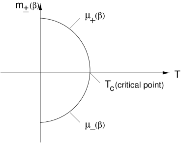
Figure 6: Spontaneous magnetization in the Ising model for $d\geq 2$.

5.2 Spin systems with continuous symmetry groups

Instead of the discrete spin variables $\sigma_{x}=\pm 1$, we consider now continuous ’spins’: $x\mapsto\varphi_{x}\in\mathbb{R}^{N},S^{N},...,$ and interactions which are invariant under a continuous symmetry group.

Let $\mu$ be a translationally invariant infinite-volume equilibrium state. Assume that the following cluster property holds for local observables $A,~{}B$ (that is, observables which depend only on finitely many spin variables)

$$\arrowvert<A\tau_{x}(B)>-<A><B>\arrowvert={\cal O}\left(\frac{1}{|x|^{\delta}}\right)~{},\qquad\delta>0~{},$$ (5.3)

where $\tau_{a}$ denotes the translation by $a$. One can prove that this implies the following, provided the interaction has finite range (this can be weakened): The equilibrium state $\mu$ is invariant under the symmetry group, if

$$\delta>d-2~{}.$$ (5.4)

For a proof, see, e.g., Ref. [8], and references therein.

Consequences

• If $d=2$ all clustering states are invariant, i.e., the continuous symmetry group $G$ cannot be spontaneously broken (Mermin-Wagner Theorem).

• Consider the case $d=3$. Then in any nonsymmetric phase the clustering cannot decay faster than $|x|^{-1}$.

• For $d=4$ (field theory) there is no mass gap in a nonsymmetric phase (otherwise there would be an exponential clustering, which is not possible). This is the Goldstone-Theorem (for lattice models).

6 Order parameters and Elitzur’s theorem for gauge theories

In the previous section we considered systems with global symmetries. A spontaneous breaking of such a symmetry is accompanied by a nonvanishing spontaneous magnetization. At first sight one expects something similar for gauge theories. However, Elitzur has shown that local quantities, like a Higgs field, which are not gauge invariant, have always vanishing mean values; that is, local observables cannot exhibit spontaneous breaking of local gauge symmetries.

Since this is quite easy to prove, I give here the details for lattice gauge models. It is instructive to consider a lattice gauge theory with the gauge group $\mathbb{Z}_{2}$, because this shows the contrast to the Ising model.

First, I need some standard notation. A field configuration is a map of bonds ($b$) into the gauge group $\mathbb{Z}_{2}$: $b\mapsto\sigma_{b}(=\pm 1)$. $\sigma_{\partial P}$ denotes the group element for a plaquette $P$. The action for a finite region $\Lambda$ of the lattice $\mathbb{Z}^{d}$ is

$$S_{\Lambda}(\{\sigma\})=-\sum_{P\subset\Lambda}\sigma_{\partial P}-h\sum_{b\subset\Lambda}\sigma_{b}~{},$$ (6.1)

where $h$ is an external ’field’. The expectation value for a local observable $A$ is

$$<A>_{\Lambda}=Z_{\Lambda}^{-1}\sum_{\{\sigma\}}A(\{\sigma\})e^{-\beta S_{\Lambda}(\{\sigma\})}~{},$$ (6.2)

where $Z_{\Lambda}$ is the partition sum

$$Z_{\Lambda}=\sum_{\{\sigma\}}e^{-\beta S_{\Lambda}(\{\sigma\})}~{}.$$ (6.3)

In sharp contrast to what happens in the Ising model, the mean value of $\sigma_{b}$ does not signal a symmetry breaking:

Theorem 5 (Elitzur)

For the expectation value $<\sigma_{b}>_{\Lambda}(h)$ we have

$$\lim_{h\downarrow 0}<\sigma_{b}>_{\Lambda}(h)=0~{}~{}\rm{uniformly~{}in~{}}\Lambda~{}\rm{and}~{}\beta~{}.$$ (6.4)

In particular, the thermodynamic limit of $<\sigma_{b}>_{\Lambda}$ vanishes for $h\downarrow 0$ (no spontaneous ’magnetization’).

Before giving the simple proof, I remark that it is easy to add a Higgs field $\phi_{x}$ to the model, and prove similarly that

$$<\phi_{x}>=0~{}.$$ (6.5)

This does, however, not exclude a Higgs phase with exponential fall off of the correlation function $<\sigma_{\partial P_{1}}\sigma_{\partial P_{2}}>$ for the gauge fields (mass generation), but (6.4) and (6.5) show that this is not signaled by local observables.

Proof of Elizur’s theorem.

We choose in (6.4) the bond variable $\sigma_{01}$ for the bond $b=<0,1>$ and estimate in

$$<\sigma_{01}>_{\Lambda}=\frac{\sum_{\{\sigma\}}\sigma_{01}\exp\left(\beta\sum_{P}\sigma_{\partial P}+\beta h\sum_{b}\sigma_{b}\right)}{\sum_{\{\sigma\}}\exp\left(\beta\sum_{P}\sigma_{\partial P}+\beta h\sum_{b}\sigma_{b}\right)}$$ (6.6)

the numerator $N$ and the denominator $D$ separately.

Consider a gauge transformation $\sigma_{ij}^{\prime}=\epsilon_{i}\sigma_{ij}\epsilon_{j}$, with $\epsilon_{i}=1$ for $i\neq 0$ and replace $\sigma_{ij}$ in $N$ and $D$ by $\epsilon_{i}\sigma_{ij}^{\prime}\epsilon_{j}$, dropping afterwards the prime of $\sigma_{ij}$ ($\sigma_{ij}\rightarrow\epsilon_{i}\sigma_{ij}\epsilon_{j}$). This can be done for $\epsilon_{0}=\pm 1$. $D$ is equal to half of the sum:

$$D=\frac{1}{2}\sum_{\epsilon_{0}=\pm 1}\sum_{\{\sigma\}}\exp\left(\beta\sum_{P}\sigma_{\partial P}+\beta h\sideset{}{{}^{\prime}}{\sum}_{b}\sigma_{b}\right)\exp\left(\epsilon_{0}\beta h\sum_{j=1}^{2d}\sigma_{0j}\right)~{},$$ (6.7)

where the prime of the sum means that the bonds $<0,j>$ must be excluded. Clearly, for $h>0$

$$D\geq\sum_{\{\sigma\}}\exp\left(\beta\sum_{P}\sigma_{\partial P}+\beta h\sideset{}{{}^{\prime}}{\sum}_{b}\sigma_{b}\right)~{}\frac{1}{2}~{}e^{-2d\beta h}~{}.$$ (6.8)

Similarly, we have for the numerator

$$|N|\leq\sum_{\{\sigma\}}\exp\left(\beta\sum_{P}\sigma_{\partial P}+\beta h\sideset{}{{}^{\prime}}{\sum}_{b}\sigma_{b}\right)~{}\frac{1}{2}~{}\left|\sum_{\epsilon_{0}=\pm 1}\epsilon_{0}\sigma_{01}\exp\left(\epsilon_{0}\beta h\sum_{j=1}^{2d}\sigma_{0j}\right)\right|~{},$$ (6.9)

and thus

$$|N|\leq\sum_{\{\sigma\}}\exp\left(\beta\sum_{P}\sigma_{\partial P}+\beta h\sideset{}{{}^{\prime}}{\sum}_{b}\sigma_{b}\right)\sinh(2d\beta h)~{}.$$ (6.10)

This gives the estimate

$$\arrowvert<\sigma_{01}>_{\Lambda}(h)\arrowvert\leq 2e^{2d\beta h}\sinh(2d\beta h)\overset{\small{(h\downarrow 0)}}{\longrightarrow}0~{},$$ (6.11)

uniformly in $\Lambda$ and $\beta$.       QED.

This argument can easily be generalized to any lattice gauge theory and any local observable which is noninvariant under the gauge group (see, e.g., [9], Chap. 6).

Elitzur’s theorem implies that possible order parameters have to be nonlocal objects. An example of such a quantity is the Wilson loop and the associated string tension.

What is the reason for this different behavior of models with local and global symmetries? Consider again the Ising model in the absence of an external field. At low temperatures, the two regions in configuration space with opposite magnetizations ${\sigma_{x}}$ and ${-\sigma_{x}}$ can only be connected by a dynamical path involving the creation of an infinite interface which costs an infinite amount of energy. Therefor the process cannot occur spontaneously. Alternatively, one can make use of a small external field which is switched off after the thermodynamic limit is taken. On the other hand, in a local gauge theory one can perform gauge transformations which act only on a finite set of basic variables on which a local ”observable” depends, and which leaves the complementary set invariant.

References

- [1] C. Truesdell, The rational mechanics of elastic or flexible bodies, 1638-1788. Leonhardi Euleri opera omnia, Serie II, Vol. 11, Teil 2; Zürich, Orell Füssli, 1960.
- [2] L.D. Landau & E.M. Lifshitz: Course of Theoretical Physics, Theory of Elasticity, Vol. 7, 3rd Edition.
- [3] J. Stillwell, Elements of Algebra, Geometry, Numbers, Equations; Springer-Verlag 1994.
- [4] S. Chandrasekhar, Newton’s Principia for the Common Reader; Clarendon Press, Oxford 1995.
- [5] S. Chandrasekhar, Ellipsoidal Figures of Equilibrium; Yale University Press 1969, Dover, New York 1987.
- [6] S. Chandrasekhar, Hydrodynamics and Hydromagnetic Stability; Clarendon Press, Oxford 1961, Dover, New York 1981.
- [7] A. Pais, Subtle Is the Lord … The Science and Life of Albert Einstein; Oxford University Press, 1982.
- [8] P.A. Martin, Il Nuovo Cimento, 68B, 302 (1982).
- [9] C. Itzykson, J.-M. Drouffe, Statistical Field Theory, Vol. 1; Cambridge University Press, 1989.