ROME1-1222/98

Heavy-heavy form factors and generalized factorization

M. Ciuchini¹, R. Contino², E. Franco², G. Martinelli²

¹ Dipartimento di Fisica, Università di Roma Tre and INFN

Sezione di Roma III, Via della Vasca Navale 84, I-00146 Rome, Italy.

² Dipartimento di Fisica, Università “La Sapienza” and INFN,

Sezione di Roma, P.le A. Moro 2, I-00185 Rome, Italy.

We reanalyze $B\to D\pi$ and $B\to KJ/\psi$ data to extract a set of parameters which give the relevant hadronic matrix elements in terms of factorized amplitudes. Various sources of theoretical uncertainties are studied, in particular those depending on the model adopted for the form factors. We find that the fit to the $B\to D\pi$ branching ratios substantially depends on the model describing the Isgur-Wise function and on the value of its slope. This dependence can be reduced by substituting the $BR(B\to D\pi)$ with suitable ratios of non-leptonic to differential semileptonic $BR$s. In this way, we obtain a model-independent determination of these parameters. Using these results, the $B\to D$ form factors at $q^{2}=M_{\pi}^{2}$ can be extracted from a fit of the $BR(B\to D\pi)$. The comparison between the form factors obtained in this way and the corresponding measurements in semileptonic decays can be used as a test of (generalized) factorization free from the uncertainties due to heavy-heavy form factor modeling. Finally, we present predictions for yet-unmeasured $D\pi$ and $DK$ branching ratios and extract $f_{D_{s}}$ and $f_{D_{s}^{*}}$ from $B\to DD_{s}$ decays. We find $f_{D_{s}}=270\pm 45$ MeV and $f_{D_{s}^{*}}=260\pm 40$ MeV, in good agreement with recent measurements and lattice calculations.

ROME1-1222/98

Oct. 1998

1 Introduction

A problem of utmost importance in $B$ phenomenology is the computation of the hadronic amplitudes: in recent years it has been realized that the full determination of the unitarity triangle from $B$ decays can hardly be carried out without an accurate knowledge of these quantities [1, 2]. Unfortunately, the computation of hadronic amplitudes requires an understanding of low-energy strong interactions which is missing at present. Even a non-perturbative approach based on first principles, such as lattice QCD, fails in computing decay amplitudes involving two or more hadrons in the final state [3].

In the absence of rigorous methods, some simplifying approaches have been developed. The most popular one consists in the factorization of matrix elements of four-fermion operators in terms of local products of two currents. In this approach, the original matrix element is computed as product of the matrix elements of the two currents. Attempts to give theoretical soundness to this procedure in the framework of the $1/N$ expansion and of the Large Energy Effective Theory (LEET) can be found in refs. [4, 5]. Unfortunately, there are many problems in both these approaches and their applicability to exclusive decays is questionable. Independently of any theoretical prejudice, there is a priori no reason for this approximation to be accurate in the case of $B$ decays. Indeed, none of the expansions developed so far was able to compute corrections to the lowest order results and estimate the size of the errors. On the other hand, the importance of controlling the theoretical uncertainties calls for some phenomenological approach to test predictions obtained using factorized amplitudes. To this end, a popular method consists in reducing the Wick contractions of matrix elements to few topologies using Fierz transformations and color rearrangement. Then, the remaining amplitudes are factorized and expressed in terms of the appropriate decay constants and/or form factors. In this procedure, some phenomenological parameters are introduced in order to account for possible deviations from factorization [1, 6, 7]. These factorization parameters, denoted as FP in the following, are meant to be fitted to experimental data.

In this paper, we introduce a parameterization of the hadronic matrix elements that extends the one of ref. [1] and allows the computation of the hadronic amplitudes relevant to Cabibbo-allowed non-leptonic $B$ decays in terms of factorized matrix elements and of three real FP. We find that, in the fit of the $BR(B\to D\pi)$ and $BR(B\to KJ/\Psi)$, there is a strong interplay between the values of the FP and the model used for the heavy-heavy form factors, more specifically on the Isgur-Wise (IW) function and its slope $\rho^{2}$ . This implies that factorization tests are obscured by our ignorance on the values of the form factors in the kinematical region relevant in non-leptonic decays ($q^{2}\ll q^{2}_{max}$). The model dependence is drastically reduced by using, in the fit, suitable ratios of semileptonic and non-leptonic $BR$s (to be introduced below) instead of the $BR(B\to D\pi)$ alone. In this way, we are able to extract (almost) model independent FP. With these FP at hand, we use then the $BR(B\to D\pi)$ to determine, within a given model, the value of $\rho^{2}$ which may be compared, as a test of factorization, to the one measured in semileptonic decays. The value of $\rho^{2}$ extracted from the fit depends, however, on the model used for the form factors. Different values of $\rho^{2}$ compensate, indeed, for the different dependence of the theoretical form factors on the momentum transfer, thus giving the same values for the matrix elements of the weak currents at low $q^{2}$. We conclude that the quantities to be compared with the corresponding ones in semileptonic decays are the form factors themselves in the region of $q^{2}$ relevant in non-leptonic decays (e.g. $q^{2}=M_{\pi}^{2}\sim 0$ for $B\to D\pi$ decays). This is a real test of factorization, free from model uncertainties. The values of the form factors extracted from our analysis are given in table 1.

Form Factor	LINSR	NRSX
$f_{+}(M_{\pi}^{2})$	0.56 [0.49–0.63]	0.57 [0.52–0.63]
$V(M_{\pi}^{2})$	0.68 [0.61–0.73]	0.75 [0.69–0.81]
$A_{0}(M_{\pi}^{2})$	0.59 [0.54–0.64]	0.58 [0.54–0.63]
$A_{1}(M_{\pi}^{2})$	0.59 [0.53–0.64]	0.56 [0.52–0.61]
$A_{2}(M_{\pi}^{2})$	0.59 [0.53–0.64]	0.54 [0.49–0.58]

Table 1: Values of $B\to D$ form factors determined by fitting the $B\to D\pi$ data with two different models, as explained in the text below. The ranges in square brackets correspond to variations of $\chi^{2}/dof$ up three times larger than its minimum. We find that form factors at $q^{2}=M_{\pi}^{2}$ already verify the kinematical relation $f_{0}=f_{+}$ and $A_{3}=A_{0}$ valid at $q^{2}=0$.

In principle, one may extract the five form factors of tab. 1 independently. However, in our analysis, all the form factors are related to the IW function through the heavy quark symmetry. Consequently, the only $B\to D$ form factor measured so far at small $q^{2}$, $f_{+}(0)$, already allows a full test of our approach. Its experimental value, $f_{+}(0)=0.66\pm 0.06\pm 0.04$ [8] is in good agreement with our findings. Measurements of the other form factors entering $B\to D^{*}$ semileptonic decays would check the relations enforced by the heavy quark symmetry.

The determination of the FP also allows us to predict several $BR$s, including $B\to DK$, which have not been measured yet. Our predictions are presented in table 2.

Finally, using ratios of non-leptonic $BR$s involving $D^{(*)}D_{s}^{(*)}$ final states and the FP and form factors from the previous fits, we extract the meson decay constants $f_{D_{s}}$ and $f_{D_{s}^{*}}$, obtaining

$$f_{D_{s}}=270\pm 45~{}\mbox{MeV},\qquad f_{D_{s}^{*}}=260\pm 40~{}\mbox{MeV},$$ (1)

in good agreement with recent experimental measurements $f_{D_{s}}=250\pm 30$ MeV [9] and lattice determinations, $f_{D_{s}}=218^{+20}_{-14}$ MeV (quenched), $f_{D_{s}}=235^{+22+17}_{-15-9}$ MeV (unquenched) [10] and $f_{D_{s}^{*}}=240\pm 20$ MeV (preliminary quenched) [11]. We also study the contribution of charming penguins [1] and discuss their effects on the predictions for the decay constants, which we find non-negligible.

The paper is organized as follows. In sect. 2 we introduce our FP and two different models for the form factors to be used in the phenomenological analysis. Section 3 contains the main results of our fits to the $B\to D\pi$ and $B\to KJ/\Psi$ branching ratios, namely the determination of the FP, the analysis of their $\rho^{2}$ dependence and the extraction of the $B\to D$ and $B\to D^{*}$ form factors at $q^{2}=M_{\pi}^{2}$. The results of these fits have been used for the predictions of yet-unmeasured $BR$s, including many $B\to DK$ modes. Finally, in sect. 4, we analyze the $B\to DD_{s}$ modes and extract $f_{D_{s}}$ and $f_{D_{s}^{*}}$, giving an estimate of the theoretical error which includes charming-penguin effects.

Channel	LINSR		NRSX		Experiment
	$[BR\times 10^{5}]$		$[BR\times 10^{5}]$		$[BR\times 10^{5}]$
$B_{d}\to\pi^{0}\bar{D}^{0}$	14	[1–58]	10	[2–27]	$<12$
$B_{d}\to\pi^{0}\bar{D}^{*0}$	15	[1–63]	13	[2–35]	$<44$
$B_{d}\to\rho^{0}\bar{D}^{0}$	6	[1–26]	7	[1–19]	$<39$
$B_{d}\to\rho^{0}\bar{D}^{*0}$	17	[2–71]	14	[2–38]	$<56$
$B_{d}\to K^{+}D^{-}$	22	[13–38]	23	[16–32]	–
$B_{d}\to K^{+}D^{*-}$	22	[14–37]	22	[16–30]	–
$B_{d}\to K^{*+}D^{-}$	53	[32–90]	53	[38–75]	–
$B_{d}\to K^{*+}D^{*-}$	67	[43–110]	64	[46–88]	–
$B^{+}\to K^{+}\bar{D}^{0}$	35	[12–54]	35	[18–45]	$29\pm 10$
$B^{+}\to K^{+}\bar{D}^{*0}$	36	[13–54]	35	[17–44]	–
$B^{+}\to K^{*+}\bar{D}^{0}$	67	[34–100]	69	[42–88]	–
$B^{+}\to K^{*+}\bar{D}^{*0}$	87	[46–126]	83	[51–104]	–
$B_{d}\to K_{0}\bar{D}^{0}$	1.4	[0.2–5.7]	1.0	[0.2–2.7]	–
$B_{d}\to K_{0}\bar{D}^{*0}$	1.5	[0.2–6.2]	1.3	[0.2–3.4]	–
$B_{d}\to K^{*0}\bar{D}^{0}$	0.6	[0.1–2.7]	0.7	[0.1–1.8]	–
$B_{d}\to K^{*0}\bar{D}^{*0}$	1.7	[0.2–7.2]	1.4	[0.2–3.6]	–

Table 2: Predictions of yet-unmeasured branching ratios.

2 Factorization, FP and form-factor models

In this section, we present our parameterization of the hadronic amplitudes and discuss its relation with other popular choices. We also introduce two different models for the form factors used in our phenomenological analysis.

Consider the matrix element of some composite operator appearing in the $\Delta B=1$ weak Hamiltonian, between the $B$ meson and two final pseudoscalar or vector mesons. In general this operator can be written as the product of two currents. If one of the currents has the correct quantum numbers to create one of the final state mesons from the vacuum, then the matrix element can be factorized. The physical idea is the following: the quark pair produced by this current acts as a color dipole, weakly interacting with the surrounding color field. If the transferred energy is large, the quark pair has no time to interact before hadronizing far from the interaction point [12].

As an example, we discuss the factorization of the amplitudes entering the decay $B_{d}\to D^{-}\pi^{+}$. In this case, the two relevant matrix elements ($\alpha$ and $\beta$ are color indices)

$$\langle D^{-}\pi^{+}|Q_{1}|B_{d}\rangle = \langle D^{-}\pi^{+}|\bar{b}_{\alpha}\gamma_{\mu}(1-\gamma_{5})c_{\beta}~{}\bar{u}_{\beta}\gamma^{\mu}(1-\gamma_{5})d_{\alpha}|B_{d}\rangle,$$

$$\langle D^{-}\pi^{+}|Q_{2}|B_{d}\rangle = \langle D^{-}\pi^{+}|\bar{b}_{\alpha}\gamma_{\mu}(1-\gamma_{5})c_{\alpha}~{}\bar{u}_{\beta}\gamma^{\mu}(1-\gamma_{5})d_{\beta}|B_{d}\rangle,$$ (2)

can be Wick-contracted according to two different topologies, that are usually denoted as connected ($CE$) and disconnected ($DE$) emissions, respectively. Color indices can be rearranged using the algebraic relation,

$$\delta_{\alpha\beta}\delta_{\rho\sigma}=\frac{1}{N}\delta_{\alpha\sigma}\delta_{\rho\beta}+2t^{a}_{\alpha\sigma}t^{a}_{\rho\beta},$$ (3)

where $N$ is the number of colors, $\delta$ is the Kronecker symbol and the $t^{a}$ are the $SU(N)$ color matrices in the fundamental representation, normalized as $tr(t^{a}t^{b})=\delta^{ab}/2$. Using this relation, one obtains

      CE $=\frac{1}{N}$ DE $+2$ octet terms  .

In the factorization limit, no gluon exchange occurs between the quark pair of the emitted meson and the other quarks, so that the octet terms vanish and the relation between $DE$ and $CE$ becomes simply $CE=DE/N$. Exact factorization is known to fail, however, in reproducing $D$ phenomenology [13]. For this reason, it is customary to introduce several phenomenological parameters to account for octet terms (and in general for the different sources of factorization violation). These parameters may be extracted from the experimental data. An example is provided by the generalized factorization of ref. [7]. In this case the relevant contractions are rewritten, without loss of generality, as

$$DE=(1+\epsilon_{1})DE_{fact}\ ,\qquad CE=\left(\frac{1}{N}+\frac{\epsilon_{8}}{1+\epsilon_{1}}\right)(1+\epsilon_{1})DE_{fact}\ ,$$ (4)

where the two parameters, $\epsilon_{1}$ and $\epsilon_{8}$, vanish in the factorization limit.

In this paper, following ref. [1], we adopt a different parameterization, given by

$$DE=\alpha DE_{fact},\qquad CE=\alpha e^{i\delta_{\xi}}\xi DE_{fact},$$ (5)

where $DE$ and $CE$ are given in terms of three real parameters $\alpha$, $\xi$ and $\delta_{\xi}$. Note that there is no inconsistency between the two parameterizations: in general, there are three real parameters, namely two moduli $|DE|$, $|CE|$, and one relative phase, $\arg(CE)-\arg(DE)$. These correspond to our three real parameters $\alpha$, $\xi$ and $\delta_{\xi}$ or to the two complex parameters $\epsilon_{1}$ and $\epsilon_{8}$ in eq. (4), one of which can always be chosen real. The relation between the two sets of parameters is given by

$$\alpha=1+\epsilon_{1},\qquad\xi e^{i\delta_{\xi}}=\frac{1}{N}+\frac{\epsilon_{8}}{1+\epsilon_{1}}.$$ (6)

As recently stressed in ref. [14], these phenomenological parameters are renormalization scale and scheme dependent, as much as the original matrix elements, since the factorized amplitudes are insensitive to both the scale and the scheme. This dependence is required to cancel the corresponding dependence in the Wilson coefficients, up to the order at which the perturbative calculation is done. Note that, in order to study the scale dependence of the parameters, the next-to-leading order (NLO) determination of the effective Hamiltonian is required. Being scheme-dependent, any physical interpretation of the “factorization scale”, namely of the renormalization scale (if it really exists) at which exact factorization holds, is meaningless. Nevertheless, the FP can be precisely extracted from data, once the renormalization scale and the scheme are fixed. Their values will depend, of course, on these choices. We will use the NDR-$\overline{\rm MS}$ NLO Wilson coefficients computed at $\mu=5$ GeV, as given in ref. [15]. In the following, it is understood that we determine $\alpha$, $\xi$ and $\delta_{\xi}$ using this choice of the scale and of the renormalization scheme.

After the introduction of the FP, the only amplitude that remains to be computed, namely

$$DE_{fact} = \langle D^{-}\pi^{+}|\bar{b}\gamma_{\mu}(1-\gamma_{5})c~{}\bar{u}\gamma^{\mu}(1-\gamma_{5})d|B_{d}\rangle|_{fact}$$ (7)

$$= \langle D^{-}|\bar{b}\gamma_{\mu}(1-\gamma_{5})c|B_{d}\rangle\langle\pi^{+}|\bar{u}\gamma^{\mu}(1-\gamma_{5})d|0\rangle~{},$$

can be easily expressed in terms of the $B\to D$ semileptonic form factors and of the decay constant $f_{\pi}$.

In this example, only left-handed currents appear. In general, considering also penguin operators, there are diagrams involving different Dirac structures, e.g. $\gamma^{\mu}(1-\gamma_{5})\otimes\gamma^{\mu}(1+\gamma_{5})$ and $(1-\gamma_{5})\otimes(1+\gamma_{5})$. In the case of interest, the right-handed current always appears in the matrix element of the emitted meson, $\langle M|\bar{q}\gamma^{\mu}(1+\gamma_{5})q^{\prime}|0\rangle$, while the current entering the other matrix element is always left-handed. Therefore only the vector or the axial current separately contributes, depending on the quantum numbers of the emitted meson. Consequently, assuming that both left-left and left-right operators can be described with the same set of FP, the relation between the corresponding matrix elements becomes trivial. Similarly, matrix elements of operators with a $(1-\gamma_{5})\otimes(1+\gamma_{5})$ Dirac structure can be connected to the current-current ones via the vector and axial vector Ward identities . In summary, using factorization, one only needs to compute matrix elements of currents, that can be expressed in terms of form factors and/or decay constants. However, these relations among insertions of different Dirac structures only hold for factorized amplitudes. By using only one set of FP, we implicitly assume that the same relations hold for the original four-fermion operator matrix elements. This simplifying assumption allows us to account for penguin-operator contributions using factorization, albeit in a model-dependent way.

In our analysis, we use the same FP for i) matrix elements connected by $SU(2)$ flavor symmetry; ii) matrix elements with the same quark content, differing only for the angular momentum of the final hadrons. The first assumption has sound phenomenological motivations; the second is reasonable since some of the differences among matrix elements with pseudoscalar and/or vector meson final states are already accounted for by factorized matrix elements.

For a generic transition $B\to P(V)$ of a $B$ going into a pseudoscalar (vector) meson of mass $M$, momentum $p$ (and polarization $\epsilon$), the form factors in the helicity basis are defined as

$$\langle P(p)|\hat{V}_{\mu}|B(p_{B})\rangle = f_{+}(q^{2})\Bigg{\{}(p+p_{B})_{\mu}-q_{\mu}\frac{M_{B}^{2}-M^{2}}{q^{2}}\Bigg{\}}+f_{0}(q^{2})q_{\mu}\frac{(M_{B}^{2}-M^{2})}{q^{2}},$$

$$\langle V(p,\epsilon)|\hat{V}_{\mu}|B(p_{B})\rangle = \frac{2i}{M_{B}+M}\varepsilon_{\mu\nu\alpha\beta}\epsilon^{*\nu}p^{\alpha}p_{B}^{\beta}V(q^{2}),$$ (8)

$$\langle V(p,\epsilon)|\hat{A}_{\mu}|B(p_{B})\rangle = 2MA_{0}(q^{2})q_{\mu}\frac{\epsilon^{*}\cdot q}{q^{2}}+A_{1}(q^{2})(M_{B}+M)\Bigg{\{}\epsilon^{*}_{\mu}-q_{\mu}\frac{\epsilon^{*}\cdot q}{q^{2}}\Bigg{\}}$$

$$\quad-\frac{A_{2}(q^{2})}{M_{B}+M}\Bigg{\{}(p_{B}+p)_{\mu}\epsilon^{*}\cdot q-q_{\mu}\frac{\epsilon^{*}\cdot q}{q^{2}}(M_{B}^{2}-M^{2})\Bigg{\}},$$

where $\hat{V}_{\mu}$ and $\hat{A}_{\mu}$ are the vector and axial currents respectively.

For heavy final mesons, the form factors can be connected to the HQET functions $\xi_{i}(y)$, see e.g. ref. [16], using the following formulas

$$\langle P(v)|\hat{V}_{\mu}|B(v_{B})\rangle = \sqrt{M_{B}M}\;\Big{\{}\xi_{+}(y)(v_{B}+v)_{\mu}+\xi_{-}(y)(v_{B}-v)_{\mu}\Big{\}},$$

$$\langle V(v,\epsilon)|\hat{V}_{\mu}|B(v_{B})\rangle = \sqrt{M_{B}M}\;\Big{\{}i\xi_{V}(y)\varepsilon_{\mu\nu\alpha\beta}\epsilon^{*\nu}v^{\alpha}v_{B}^{\beta}\Big{\}},$$ (9)

$$\langle V(v,\epsilon)|\hat{A}_{\mu}|B(v_{B})\rangle = \sqrt{M_{B}M}\;\Big{\{}\xi_{A_{1}}(y)(y+1)\epsilon^{*}_{\mu}$$

$$\quad-\xi_{A_{2}}(y)(\epsilon^{*}\cdot v_{B})v_{B\,\mu}-\xi_{A_{3}}(y)(\epsilon^{*}\cdot v_{B})v_{\mu}\Big{\}},$$

where $v_{B}$ and $v$ are the 4-velocities of the initial and final meson respectively and

$$y\equiv v_{B}\cdot v=\frac{M_{B}^{2}+M^{2}-q^{2}}{2M_{B}M}.$$ (10)

In the heavy quark limit, the functions $\xi_{i}(y)$ are all related to the IW function $\xi(y)$

$$\xi_{+}=\xi_{V}=\xi_{A_{1}}=\xi_{A_{3}}=\xi(y),\qquad\xi_{-}=\xi_{A_{2}}=0,$$ (11)

with the normalization of $\xi$ fixed by the heavy quark symmetry, $\xi(1)=1$. The $\xi_{i}(y)$ can be written as

$$\xi_{i}(y)=\Big{\{}\alpha_{i}+\frac{\alpha_{s}(\bar{m})}{\pi}\beta_{i}(y)+\gamma_{i}(y)\Big{\}}\,\xi(y),$$ (12)

where the functions $\beta_{i}(y)$ and $\gamma_{i}(y)$ take into account the perturbative ${\cal O}(\alpha_{s})$ corrections and the ${\cal O}(1/m)$ terms respectively . Following ref. [17], we used for $\bar{m}$ the reduced charm-bottom mass i.e. $\bar{m}=2.26$ GeV.

We are now ready to introduce the two models that we will use in order to study the form-factor dependence of the FP. We denote these models as LINSR and NRSX:

• LINSR: the first model uses the heavy-heavy form factors defined in eq. (12), taking the $\beta_{i}(y)$ from ref. [17] and neglecting the ${\cal O}(1/m)$ corrections, i.e. $\gamma_{i}(y)=0$. For the IW function, the simplest form is assumed, namely

  $$\xi(y)=1-\rho^{2}(y-1)\ .$$ (13)

  For the heavy-light form factors, LINSR uses those computed with light-cone QCD sum rules [18].

• NRSX: the second model is the one defined in ref. [19] and makes use of the functions $\beta_{i}(y)$ and $\gamma_{i}(y)$ calculated in refs. [16] and [17], respectively. The IW function is obtained using a relativistic oscillator model, which gives

  $$\xi(y)=\frac{2}{y+1}\exp\bigg{\{}-A\;\frac{y-1}{y+1}\bigg{\}},$$ (14)

  where $A=2\rho^{2}-1$. Concerning the heavy-light form factors, NRSX improves the old WSB model [20] by implementing, for $q^{2}\sim q^{2}_{max}$, the expected heavy quark scaling laws, see ref. [19] for details.

We end this section by spending a word of comment about the parameter $\rho^{2}$ entering eqs. (13) and (14). In both models, $\rho^{2}$ is defined as the slope of the IW function at the zero-recoil point (i.e. $y\equiv v_{B}\cdot v=1$), namely

$$\rho^{2}\equiv-\frac{d}{dy}\xi(y)\bigg{|}_{\,y=1}.$$ (15)

The value of $\rho^{2}$ is related to the semileptonic differential rate for $B\to D^{*}l\nu$,

$$\frac{d\Gamma(B\to D^{*}l\nu)}{dy} = \frac{G_{F}^{2}}{48\pi^{3}}M_{D^{*}}^{3}(M_{B}-M_{D^{*}})^{2}\sqrt{y^{2}-1}(y+1)^{2}$$ (16)

$$\times\bigg{[}1+\frac{4y}{y+1}\frac{1-2yr+r^{2}}{(1-r)^{2}}\bigg{]}|V_{cb}|^{2}{\cal F}(y)^{2},$$

where $r\equiv M_{D^{*}}/M_{B}$ and ${\cal F}(y)$ is an effective semileptonic form factor. The latter is a calculable function of the $\xi_{i}(y)$s. To make contact with experiments, one defines the slope

$$\hat{\rho}^{2}\equiv-\frac{1}{{\cal F}(1)}\frac{d}{dy}{\cal F}(y)\bigg{|}_{\,y=1},$$ (17)

which can be extracted from the measurement of the semileptonic differential rate.

The relation between the experimental slope $\hat{\rho}^{2}$ and the theoretical parameter $\rho^{2}$ depends on the model used for the calculation of eq. (16). We found

LINSR $$\rho^{2}=\;\hat{\rho}^{2}-0.13,$$

NRSX $$\rho^{2}=\;\hat{\rho}^{2}+0.084,$$ (18)

to be compared with the results of ref. [21], $\rho^{2}=\;\hat{\rho}^{2}-(0.14\pm 0.02)+{\cal O}(1/m)$ and $\rho^{2}=\;\hat{\rho}^{2}\pm 0.2$ respectively.

In the next section, we will study the dependence of our results on the physical slope $\hat{\rho}^{2}$, rather than $\rho^{2}$.

3 Fitting Cabibbo-allowed decay modes

	Channel	$BR$ $\times 10^{5}$
	$\star$ $B_{d}\to\pi^{+}D^{-}$	$300\pm 40$
	$\star$ $B_{d}\to\pi^{+}D^{*-}$	$276\pm 21$
	$\star$ $B_{d}\to\rho^{+}D^{-}$	$790\pm 140$
	$\star$ $B_{d}\to\rho^{+}D^{*-}$	$670\pm 330$
	$B_{d}\to D_{s}^{+}D^{-}$	$800\pm 300$
Type I	$B_{d}\to D_{s}^{+}D^{*-}$	$960\pm 340$
$\propto|a_{1}|^{2}$	$B^{+}\to D_{s}^{+}\bar{D}^{0}$	$1300\pm 400$
	$B^{+}\to D_{s}^{+}\bar{D}^{*0}$	$1200\pm 500$
	$B_{d}\to D_{s}^{*+}D^{-}$	$1000\pm 500$
	$B_{d}\to D_{s}^{*+}D^{*-}$	$2000\pm 700$
	$B^{+}\to D_{s}^{*+}\bar{D}^{0}$	$900\pm 400$
	$B^{+}\to D_{s}^{*+}\bar{D}^{*0}$	$2700\pm 1000$
	$B_{d}\to K^{0}J/\psi$	$89\pm 12$
Type II	$B_{d}\to K^{*0}J/\psi$	$135\pm 18$
$\propto|a_{2}|^{2}$	$B^{+}\to K^{+}J/\psi$	$99\pm 10$
	$B^{+}\to K^{*+}J/\psi$	$147\pm 27$
	$\star$ $B^{+}\to\pi^{+}\bar{D}^{0}$	$530\pm 50$
Type III	$\star$ $B^{+}\to\pi^{+}\bar{D}^{*0}$	$460\pm 40$
$\propto|x_{1}a_{1}+x_{2}a_{2}|^{2}$	$\star$ $B^{+}\to\rho^{+}\bar{D}^{0}$	$1340\pm 180$
	$\star$ $B^{+}\to\rho^{+}\bar{D}^{*0}$	$1550\pm 310$

$q^{2}$	$\frac{d}{dq^{2}}BR(B\to D^{*}l^{+}\nu)(GeV^{-2})$	$\frac{d}{dq^{2}}BR(B\to Dl^{+}\nu)(GeV^{-2})$
$m^{2}_{\pi}$	$(0.237\pm 0.026)\times 10^{-2}$	$(0.35\pm 0.06)\times 10^{-2}$
$m^{2}_{\rho}$	$(0.250\pm 0.030)\times 10^{-2}$	$(0.33\pm 0.06)\times 10^{-2}$
$m^{2}_{D_{s}}$	$(0.483\pm 0.033)\times 10^{-2}$	–
$m^{2}_{D_{s}^{*}}$	$(0.507\pm 0.035)\times 10^{-2}$	–

Table 3: Experimental branching ratios [8, 22, 23] of decay modes to be used in the fit of the parameters $\alpha$, $\xi$ and $\delta_{\xi}$. The classification of non-leptonic channels according to their dependence on $a_{1}$ and $a_{2}$ is also shown. The channels marked with $\star$ have been used for the fit of the ratios defined in eq. (20).

This section contains the results of our phenomenological analysis of Cabibbo-allowed $B$ decays, focused on the rôle of heavy-heavy form factors. We proceed as follows:

• we show that the best fit to the $BR(B\to D\pi)$ and $BR(B\to KJ/\Psi)$ is obtained for different values of $\hat{\rho}^{2}$, depending on the model used for computing heavy-heavy form factors;

• we use the ratios $R_{\pi}(B\to D\pi)$ introduced in ref. [24], see below, and show that, by using them instead of the $BR(B\to D\pi)$, it is possible to fit the FP (almost) independently of $\hat{\rho}^{2}$. This method gives our best determination of the FP, free from theoretical uncertainties coming from the assumptions made for the heavy-heavy form factors;

• using the ($\hat{\rho}^{2}$-independent) FP, we perform a fit to the $BR(B\to D\pi)$ in order to extract a preferred range for the value of $\hat{\rho}^{2}$; the results are model dependent, in agreement with our first finding;

• we show that the different ranges of $\hat{\rho}^{2}$ actually correspond to the same values of the relevant form factors at $q^{2}=M_{\pi}^{2}\sim 0$. Using the HQET, the latters can be determined by factorization applied to $B\to D\pi$ decays and may be compared with direct measurements from semileptonic decays.

The relevant decay modes which we use in the fits are listed in tab. 3. It is well known that, in the factorization approximation, only two combinations of $DE$ and $CE$ appear in the amplitudes of these decays. This feature is taken into account by the parameters $a_{1}$ and $a_{2}$ introduced by BSW [6]. The relation between $a_{1}$ and $a_{2}$ and our parameters is given by

$$a_{1}=\alpha\left(C_{2}+\xi e^{i\delta_{\xi}}C_{1}\right),\qquad a_{2}=\alpha\left(C_{1}+\xi e^{i\delta_{\xi}}C_{2}\right)$$ (19)

where $C_{1}$ and $C_{2}$ are the Wilson coefficients of the operators defined in eq. (2) . In tab. 3, the decay modes are organized according to the standard classification in three classes. Amplitudes of Type I, II and III decay modes are proportional to $|a_{1}|$, $|a_{2}|$ and $|x_{1}a_{1}+x_{2}a_{2}|$ respectively, where $x_{i}$ are generic, process-dependent coefficients.

Given the structure of the amplitudes, we have to fit decay modes of all the three classes in order to fully determine the FP. Note that the three classes have a different dependence on the form-factors. While Type-II decays always involve a heavy-light transition, heavy-heavy form factors enter Type-I modes only. The latter is a general feature, since Type-I transitions are always driven by charged currents and are therefore proportional to $a_{1}$. In general Type-III modes involve transitions of both sorts. In our parameterization, Type-I modes essentially fix $\alpha$, while both Type II and III are needed to constrain $\xi$ and $\delta_{\xi}$.

$\frac{\chi^{2}}{dof}$

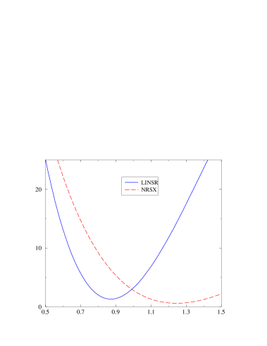
$\hat{\rho}^{2}$

Figure 1: $\hat{\rho}^{2}$ dependence of the minimum $\chi^{2}/dof$ from the fit of $\xi$ to $BR(B\to D\pi)$ and $BR(B\to KJ/\Psi)$ assuming $\alpha=1$ and $\delta_{\xi}=0$. Both LINSR and NRSX results are shown.

Contrary to the common wisdom, the assumptions made on the momentum dependence of the heavy-heavy form factors introduce large uncertainties in the determination of the FP from this fit. This is more easily shown fitting only the effective number of colour as done in the old literature . In our parametrization this corresponds to assume $\alpha=1$ and $\delta_{\xi}=0$ and to fit $\xi$ only. The result of this fit is shown in fig. 1, where minimum values of $\chi^{2}/dof$ from the fit of $\xi$ to the $BR(B\to D\pi)$ and to the $BR(B\to KJ/\Psi)$ are plotted as function of $\hat{\rho}^{2}$. It is apparent that the best fit is obtained for quite different values of $\hat{\rho}^{2}$, and corresponds to different values of $\xi$, depending on the model used to compute the heavy-heavy form factors. Consequently, in general, the FP fitted using $BR$s at fixed $\hat{\rho}^{2}$, as usually done in the literature, suffer from a large theoretical error, which was previously hidden in the choice of a specific model when fitting the data. The second important remark is that a comparison of the value of $\hat{\rho}^{2}$, the “physical” slope measured in semileptonic decays, with that extracted from non-leptonic decays is not a good test of factorization since, in the latter case, the result is model dependent.

To circumvent this problem in the determination of the FP, instead of the Type-I and Type-III $BR$s, we fit the ratios

$$R_{M}(B\to D^{(*)}M)=\frac{BR(B\to D^{(*)}M)}{\frac{d}{dq^{2}}BR(B\to D^{(*)}l\nu)|_{q^{2}=m_{M}^{2}}},$$ (20)

where $M=\pi,D_{s},\dots$ is the emitted meson. The advantage of using eq. (20) is that in these ratios the heavy-heavy form factor dependence drops out completely for Type-I decays and is strongly reduced for Type III. In practice, we used the ratios corresponding to the non-leptonic decays marked with $\star$ in table 3. In the fit, besides the ratios $R_{M}$ for Type-I and Type-III, we also use all the $BR$s of the Type-II decays.

LINSR		$\hat{\rho}^{2}=0.80$	$\hat{\rho}^{2}=0.90$	$\hat{\rho}^{2}=1.00$
$R_{\pi}(B\to D\pi)$	$\chi^{2}/dof$	$1.36$	$1.36$	$1.36$
Type I	$\alpha$	$1.02$	$1.02$	$1.02$
+	$\xi$	$0.45$	$0.45$	$0.45$
$BR(B\to KJ/\psi)$	$\delta_{\xi}$	$0.00$	$0.00$	$0.00$
$R_{\pi}(B\to D\pi)$	$\chi^{2}/dof$	$1.40$	$1.39$	$1.42$
Type I+III	$\alpha$	$1.05$	$1.04$	$1.03$
+	$\xi$	$0.44$	$0.44$	$0.44$
$BR(B\to KJ/\psi)$	$\delta_{\xi}$	$0.00$	$0.00$	$-0.26$

NRSX		$\hat{\rho}^{2}=1.25$	$\hat{\rho}^{2}=1.35$	$\hat{\rho}^{2}=1.45$
$R_{\pi}(B\to D\pi)$	$\chi^{2}/dof$	$0.39$	$0.39$	$0.39$
Type I	$\alpha$	$1.01$	$1.01$	$1.01$
+	$\xi$	$0.38$	$0.38$	$0.38$
$BR(B\to KJ/\psi)$	$\delta_{\xi}$	$0.00$	$0.00$	$0.00$
$R_{\pi}(B\to D\pi)$	$\chi^{2}/dof$	$0.71$	$0.70$	$0.68$
Type I+III	$\alpha$	$1.04$	$1.04$	$1.03$
+	$\xi$	$0.38$	$0.38$	$0.38$
$BR(B\to KJ/\psi)$	$\delta_{\xi}$	$0.00$	$0.00$	$0.00$

Table 4: Results of the fit using $D\pi$ semileptonic ratios and $BR(B\to KJ/\Psi)$ for three different values of the slope $\hat{\rho}^{2}$ and the two form-factor models, LINSR and NRSX, described in the text. For each model, two fits have been performed, the difference being the inclusion of Type-III $D\pi$ modes, which introduce some $\hat{\rho}^{2}$ dependence.

The results of the fit are shown in tab. 4 for NRSX and LINSR. We do not include the $D^{(*)}D_{s}^{(*)}$ modes for two reasons: on the one hand, their contribution to the total $\chi^{2}$ is suppressed by the large experimental errors in the measured $BR$s; on the other, we want to use them to extract the decay constants $f_{D_{s}}$ and $f_{D_{s}^{*}}$.

For both choices of form factors, we give the results of two different fits: the first includes all types of decays and determines the FP $\alpha$, $\xi$ and $\delta_{\xi}$. It retains, however, a small residual dependence on heavy-heavy form factors, i.e. on $\hat{\rho}^{2}$. The second is a fit to Type-I and -II channels only, which is totally independent of $\hat{\rho}^{2}$. The results are quite close. Note that the second fit only involves two combinations of the three FP. As a consequence we have to fix one parameter in order to extract the other two: we choose to put $\delta_{\xi}=0$, quite consistently with what has been found with the first fit. As a consistency check, we have also verified that different values of $\delta_{\xi}$ do not change appreciably the results . In tab. 4 we show the fitted values of the FP for several choices of $\hat{\rho}^{2}$, for both NRSX and LINSR. As mentioned above, the results turn out to be, within a given model, independent of $\hat{\rho}^{2}$.

$\hat{\rho}^{2}$

$\xi$

Figure 2: Contour plots of $\chi^{2}/dof$ in the plane $(\xi,\hat{\rho}^{2})$, obtained from a two-parameter fit to the non-leptonic $B\to D\pi$ decays. The other parameters ($\alpha$ and $\delta_{\xi}$) have been fixed by the fit of tab. 4 in a $\hat{\rho}^{2}$-independent way. The solid curves refer to LINSR, the dashed ones to NRSX. The different contours correspond to $\chi^{2}/dof=(1.5,2,3)\times\chi^{2}_{min}/dof$.

Having fitted the FP in a $\hat{\rho}^{2}$-independent way, we now use the $BR(B\to D\pi)$ to extract from the data a preferred range of $\hat{\rho}^{2}$. Notice that $\delta_{\xi}$ is not a critical parameter, since the results of the fits are not very sensitive to its value, and that the values of $\alpha$ and $\hat{\rho}^{2}$ are trivially correlated, because the amplitudes only depend on the product of $\alpha$ with the effective form factors at $q^{2}\sim 0$. Therefore we choose to perform a two-parameter fit of $\xi$ and $\hat{\rho}^{2}$ using the $BR(B\to D\pi)$, at fixed values of $\delta_{\xi}$ and $\alpha$, as extracted from the previous fit of tab. 4. In this way, we can study the correlations in the $(\xi$–$\hat{\rho}^{2})$ plane and check the consistency of the determination of $\xi$ using different fitting procedures.

Figure 2 shows the contour plots of $\chi^{2}/dof$ in the $(\xi,\hat{\rho}^{2})$ plane for NRSX and LINSR. The fitted value of $\xi$ is consistent with tab. 4 and the preferred $\hat{\rho}^{2}$ is larger using NRSX than LINSR. Moreover, the LINSR $BR$s are steeper functions of $\hat{\rho}^{2}$, consistently with fig. 1. This observation justifies the choice of the set of values of $\hat{\rho}^{2}$ used in tab. 4.

It is not surprising that the fit to the $BR(B\to D\pi)$ gives values of $\hat{\rho}^{2}$ which are model dependent. The fit only fixes the values of the relevant heavy-heavy form factors $f_{i}=f_{+},A_{0},\dots$ at $q^{2}=M_{\pi}^{2}\sim 0$ . These form factors can be expressed in terms of the $\xi_{i}$s at $q^{2}\sim 0$ which, in turn, are related to the IW function $\xi(y)$ by heavy quark symmetry, see eq. (12). The relation between the fitted form factors at $q^{2}=M_{\pi}^{2}$ and the values of $\xi_{i}(1)$, which are fixed by the HQET, depends on the functional form adopted for the IW function $\xi(y)$ and on the value of $\rho^{2}$. Thus different values of $\hat{\rho}^{2}$ are obtained by fitting the data with different models. In particular, we find that the main difference between NRSX and LINSR relies on the choice of the IW function, eqs. (13) and (14), rather than in the inclusion of $1/m$ corrections. Plotting the results of the fit in the planes $(\xi,f_{i})$, through eqs. (8)–(12), we obtain almost the same determination of the $f_{i}(M_{\pi}^{2})$ with both NRSX and LINSR, as shown in figs. 3 and 4. Although we have considered only two models in the present study, we believe that this result is quite general.

We stress again that constraints on the heavy-heavy form factors can only be obtained by combining the results of two independent fits: the first which fixes the FP using the ratios $R_{\pi}$, that are essentially independent on the model used to calculate the form factors, and the second which fixes the form factors using the $BR(B\to D\pi)$ at fixed values of the FP.

$f_{+}(M_{\pi}^{2})$

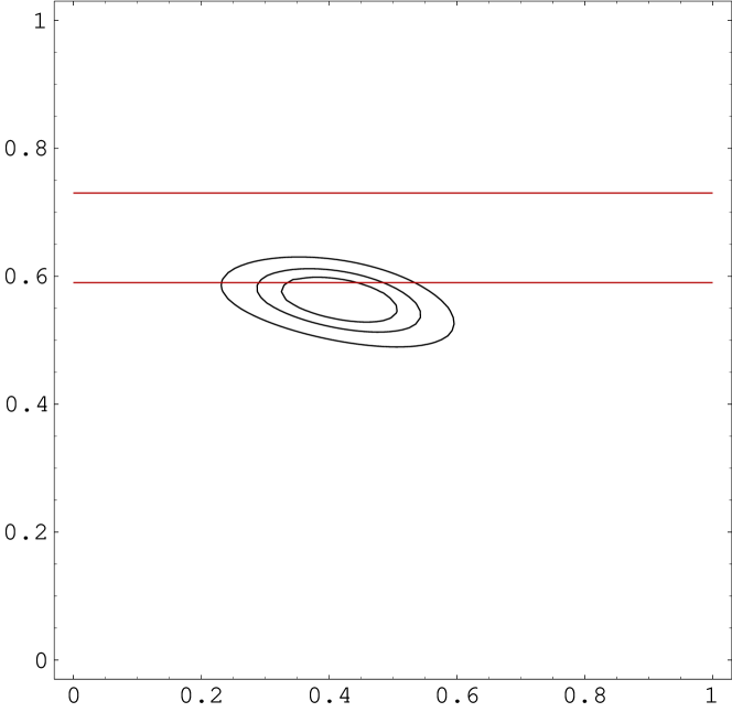
$\xi$

$f_{+}(M_{\pi}^{2})$

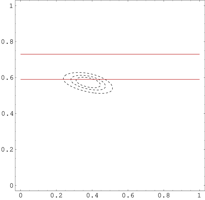
$\xi$

$V(M_{\pi}^{2})$

$\xi$

$V(M_{\pi}^{2})$

$\xi$

Figure 3: Determination of various $B\to D\pi$ form factors at $q^{2}=M_{\pi}^{2}$ as functions of $\xi$. These plots are obtained from fig. 2 using the relations connecting heavy-heavy form factors to the Isgur-Wise function, eqs. (8)–(12). LINSR (NRSX) form factors are shown in the left (right) column. The different contours correspond to $\chi^{2}/dof=(1.5,2,3)\times\chi^{2}_{min}/dof$.

$A_{0}(M_{\pi}^{2})$

$\xi$

$A_{0}(M_{\pi}^{2})$

$\xi$

$A_{1}(M_{\pi}^{2})$

$\xi$

$A_{1}(M_{\pi}^{2})$

$\xi$

$A_{2}(M_{\pi}^{2})$

$\xi$

$A_{2}(M_{\pi}^{2})$

$\xi$

Figure 4: The same plots as in fig. 3 for $A_{0}$, $A_{1}$ and $A_{2}$.

The comparison of the heavy-heavy form factors directly measured in semileptonic decays at $q^{2}=M_{\pi}^{2}\sim 0$ with the results in figs. 3 and 4, and table 1, is a real test of generalized factorization in $B\to D\pi$ decays, independently on the choice of the IW function and of the value of $\hat{\rho}^{2}$. This checks the assumptions we made for computing hadronic matrix elements as described in the previous sections. Since we use the HQET relations coming from eq. (12), we are left with only one independent form factor, namely the IW function. Therefore the only form factor directly measured at $q^{2}=0$, $f_{+}(0)$, already allows a test of our approach. Its value, $f_{+}(0)=0.66\pm 0.06\pm 0.04$ [8], showed as a band in the upper plots of fig. 3, agrees well with the result of the fit. The extraction of the other form factors at $q^{2}=0$ from the CLEO data is under way [25] and would allow a check of the HQET relations among $B\to D$ form factors near the maximum recoil point. Notice that, at least in principle, the fitting procedure described in this section could be used to extract independently the values of all the form factors at $q^{2}=M_{\pi}^{2}$, just including them among the FP. In this case, the comparison of each form factor with the measurements from semileptonic decays would be a test of generalized factorization, independent of the HQET relations eq. (12). Unfortunately the present accuracy of the data does not allow a separate determination of the different form factors.

From the discussion above, we conclude that the HQET-inspired parameterization of the heavy-heavy form factors in terms of their value at $q^{2}_{max}$ and of the slope $\hat{\rho}^{2}$, which is commonly adopted by experimental collaborations and successfully applied to semileptonic decays, is not the most appropriate choice for the factorization analysis of non-leptonic decays.

With the results for the FP given in (21), we can predict $BR$s of yet-unmeasured decay channels, having one $D$ and one light meson in the final state. We list our predictions in tab. 2, where the ranges in square brackets give an estimate of the theoretical uncertainties. They were found by allowing values of $\chi^{2}/dof$ up to three times larger than the minimum. Flavor $SU(3)$ symmetry justifies the use of parameters obtained from $B\to D\pi$ and $B\to KJ/\Psi$ decays to the decays listed in table 2. Large flavour effects are unlikely, since the factorized amplitudes already account for some $SU(3)$ breaking.

Finally, we summarize the result of our fits of the FP by quoting their best values and ranges of variation, obtained by allowing values of $\chi^{2}/dof$ up to three times larger than the minimum. The comparison between the two different models, NRSX and LINSR, gives us an estimate of the theoretical uncertainties due to the form-factor model dependence. As discussed before, these FP parameters are those obtained using the coefficients functions computed at the NLO in the $\overline{\rm MS}$ scheme with $\mu=5$ GeV. We obtain

LINSR NRSX

$$\alpha$$ 1.04 [0.9–1.2] 1.04 [1.0–1.1]

0.44 [0.2–0.5] 0.38 [0.2–0.4]

0.0 [-1.5–1.5] 0.00 [-1.0–1.0]

1.04 [0.9–1.3] 1.05 [1.0–1.2]

0.31 [0.0–0.7] 0.25 [0.0–0.4]

1.4 [1.4–4.2] 0.7 [0.7–2.1]

0.91 [0.8–1.0] 1.34 [1.1–1.5]

(21)

For the sake of comparison with previous literature, we have also shown the values of $|a_{1}|$ and $|a_{2}|$, computed using eq. (19). It is worth noticing that exact factorization, namely $\alpha=1$, $\xi=1/3$ and $\delta_{\xi}=0$, would give values of $\chi^{2}/dof$ $3$–$4$ times larger than the fits which use the generalized factorization, for both the models considered here.

4 Decay constants from $DD_{s}$ decays

In this section, we extract the meson decay constants $f_{D_{s}}$ and $f_{D_{s}^{*}}$ and compare the results with available measurements and lattice results.

We consider the semi-leptonic ratios $R_{D_{s}}(B\to D^{(*)}D_{s}^{+})$ and $R_{D_{s}^{*}}(B\to D^{(*)}D_{s}^{*+})$, introduced in the previous section, and define the non-leptonic ratios [7]

$$R^{P}_{D_{s}}(B\to D^{(*)}D_{s}^{+}) = \frac{BR(B\to D^{(*)}D_{s}^{+})}{BR(B\to D^{(*)}\pi^{+})},$$

$$R^{V}_{D_{s}^{*}}(B\to D^{(*)}D_{s}^{*+}) = \frac{BR(B\to D^{(*)}D_{s}^{*+})}{BR(B\to D^{(*)}\rho^{+})}.$$ (22)

Up to color-suppressed terms, the factorized amplitudes of the decay modes considered here are proportional to $f_{D_{s}}/f_{\pi}$ or to $f_{D^{*}_{s}}/f_{\rho}$. Whereas the ratios $R_{M}$ of eq. (20) are defined in such a way that the main form-factor dependence drops out, in the non-leptonic ratios of eqs. (22), the form factors appearing in the numerator and denominator are evaluated at different $q^{2}$ and do not cancel out. In this case, however, it is the dependence on the FP that tends to cancel, as long as penguin contributions are neglected. The non-leptonic ratios above are exactly independent of $\xi$ and $\delta_{\xi}$ only if charged $B^{+}$ decays are not considered, as done in ref. [7]. In our case, we prefer to double the number of channels in the fit, by including charged $B^{+}$ decays, at the cost of introducing a small dependence on FP and on the $D^{(*)}$ decay constants, both appearing in color suppressed terms in the decay amplitudes. We take $f_{D}=200$ MeV and $f_{D^{*}}=220$ MeV [26].

In general, all $DD_{s}$ modes suffer from a further theoretical error. This uncertainty originates from using the same FP, obtained from the fit of sec. 3, in the calculation of the relevant $BR$s entering the non-leptonic ratios. Since in $DD_{s}$ decays, the emitted meson is heavy, one may expect, according to the LEET approach, larger violations to the factorization limit. In other words, in this case the FP may significantly differ from those fixed by the $D\pi$ and $KJ/\Psi$ modes. This is a further source of theoretical uncertainty, which we are not able to estimate at present.

Using the the semileptonic ratios $R_{D_{s}}(B\to D^{(*)}D_{s}^{+})$ and $R_{D_{s}^{*}}(B\to D^{(*)}D_{s}^{*+})$ and the non-leptonic ratios of eqs. (22), the form factors determined from the fit to the $BR(B\to D\pi)$ and the FP from (21), we have extracted $f_{D_{s}}$ and $f_{D_{s}^{*}}$. Results are collected in tab. 5, where we have separately shown the uncertainties coming from the experimental errors on the $BR$s and from the errors on the FP. As before, in order to estimate this source of theoretical uncertainty, we present results obtained using both LINSR and NRSX.

From tab. 5, we quote

$$f_{D_{s}}=270\pm 35~{}\mbox{MeV},\qquad f_{D_{s}^{*}}=260\pm 30~{}\mbox{MeV},$$ (23)

where the errors indicatively account for all the sources of uncertainty.

The value obtained for $f_{D_{s}}$ is in reasonable agreement with the data [9], $f_{D_{s}}=250\pm 30$ MeV, and with the lattice results $f_{D_{s}}=218^{+20}_{-14}$ MeV (quenched), $235^{+22+17}_{-15-9}$ MeV (unquenched) [10], although within large experimental and theoretical uncertainties. Our prediction for $f_{D_{s}^{*}}$ is in good agreement with the quenched lattice determination, $f_{D_{s}^{*}}=240\pm 20$ MeV [11].

	LINSR		NRSX
MeV	semileptonic	nonleptonic	semileptonic	nonleptonic
$f_{D_{s}}$	$304\pm 42\pm 47$	$253\pm 24\pm 35$	$297\pm 41\pm 26$	$267\pm 25\pm 21$
$f_{D_{s}^{*}}$	$277\pm 36\pm 43$	$250\pm 31\pm 16$	$274\pm 36\pm 24$	$261\pm 32\pm 9$

Table 5: Decay constants extracted from both semileptonic and non-leptonic ratios, eqs. (20) and (22). Both LINSR and NRSX results are shown. The first error comes from the experimental ones on the BRs, while the second is a “theoretical” error obtained by varying the FP in a range corresponding to values of $\chi^{2}/dof$ up to three times larger than the minimum one.

Comparing the NRSX results of tab. 5 with the analysis of ref. [7], one finds differences of the order of $10$–$15\%$. Besides our inclusion of the charged decay modes, this difference arises because we take into account contributions from penguin operators, which were neglected in ref. [7]. These contributions amount up to $20\%$ in some channels, in particular to those used to determine $f_{D_{s}}$. For this reason, it is worth testing the effect of charming-penguin contractions in the determination of the leptonic decay constants. We parameterize the effects of charming penguins as in ref. [1], by using two real quantities $\eta_{L}$ and $\delta_{L}$, denoting the relative size and the phase of the charming-penguin amplitudes with respect to the corresponding emission ones. In fig. 5, we plot $\delta f_{D_{s}}=f_{D_{s}}(\eta_{L},\delta_{L})/f_{D_{s}}(0,0)-1$ as a function of $\eta_{L}$ for various choices of $\delta_{L}$, using NRSX. For $\eta_{L}\sim 0.2$–$0.3$ and $\delta_{L}\sim\pi$, as suggested by $B\to K\pi$ decays [1], $|\delta f_{D_{s}}|$ is about $20\%$, larger than the (previously) estimated theoretical error on $f_{D_{s}}$. Of course, there is no compelling theoretical reason to use parameters extracted from $K\pi$ modes in this analysis. This exercise shows, however, that penguin effects are not negligible and should be included, at least as further source of theoretical uncertainty, at the level of 10%, in addition to the one in eq. (23).

$\delta f_{D_{s}}$

$\eta_{L}$

Figure 5: Charming penguin effect on the determination of $f_{D_{s}}$ from semileptonic ratios using NRSX. The difference $\delta f_{D_{s}}=f_{D_{s}}(\eta_{L},\delta_{L})/f_{D_{s}}(0,0)-1$ is plotted as a function of $\eta_{L}$ at different values of $\delta_{L}$.

5 Conclusions

In this paper, we have introduced a parameterization of the hadronic matrix elements, that generalizes the one of ref. [1] and express the amplitudes relevant to the calculation of Cabibbo-allowed non-leptonic $B$ decays in terms of factorized matrix elements and three real parameters $\alpha$, $\xi$ and $\delta_{\xi}$. We have shown the connection of our parameterization with the generalized factorization of ref. [7]. In order to fix these parameters, we have reanalized $B\to D\pi$ and $B\to KJ/\Psi$ data.

We have found that the fit to $B\to D\pi$ decays substantially depends on the model describing the Isgur-Wise function $\xi$ and on the value of its slope. This dependence has been drastically reduced by fitting the ratios in eq. (20). We have shown that, once that the FP are fixed in this way, a best fit to the non-leptonic $BR(B\to D\pi)$ determines the values of heavy-heavy form factors at $q^{2}=M_{\pi}^{2}\sim 0$. This provides a costraint on the HQET models which are currently used for the heavy-heavy form factors. We have shown that, in general, different models require different values of $\hat{\rho}^{2}$ to reproduce the fitted values of the form factors. Consequently, a meaningful test of factorization is only provided by the comparison of the values of the form factors extracted from non-leptonic decays with those directly measured, at small values of $q^{2}$, in semileptonic decays. The only form factor directly measured at $q^{2}=0$, $f_{+}(0)=0.66\pm 0.06\pm 0.04$ [8], is in good agreement with our finding, suggesting that the generalized factorization works well in the case of $B\to D\pi$ decays.

Our best determination of the FP can be found in (21), where an estimate of the theoretical uncertainties is also given. Using these FP, we have also presented a set of predictions for the $BR$s of yet-unmeasured $B$ decays, including $D\pi$, $D\rho$, $DK^{(*)}$ modes, see tab. 2.

Finally, using non-leptonic ratios of eqs. (20) and (22), we have extracted the charmed meson decay constants from the $BR(B\to DD_{s})$, finding

$$f_{D_{s}}=270\pm 45~{}\mbox{MeV},\qquad f_{D_{s}^{*}}=260\pm 40~{}\mbox{MeV},$$ (24)

where errors indicatively account for all sources of uncertainty present in the fit, including charming penguins.

References

-
[1]
M. Ciuchini, E. Franco, G. Martinelli, and L. Silvestrini,
Nucl. Phys. B501 (1997) 271;
M. Ciuchini et al., Nucl. Phys. B512 (1998) 3. -
[2]
J.-M. Gérard and J. Weyers, UCL-IPT-97-18 [hep-ph/9711469];
M. Neubert, Phys. Lett. B424 (1998) 152;
A.F. Falk, A.L. Kagan, Y. Nir, and A.A. Petrov, Phys. Rev. D57 (1998) 4290;
D. Atwood and A. Soni, Phys. Rev. D58 (1998) 036005;
for a review, see e.g. R. Fleischer, Int. J. Mod. Phys. A12 (1997) 2459. - [3] L. Maiani and M. Testa, Phys. Lett. B245 (1990) 585.
- [4] A.J. Buras, J.-M. Gerard, and R. Ruckl, Nucl.Phys. B268 (1986) 16.
- [5] M.J. Dugan and B. Grinstein, Phys. Lett. B255 (1991) 583.
- [6] M. Bauer, B. Stech, and M. Wirbel, Z. Phys. C34 (1987) 103.
- [7] M. Neubert and B. Stech, CERN-TH/97-99, [hep-ph/9705292], to appear in “Heavy Flavours II”, edited by A.J. Buras and M. Lindner.
- [8] T. Bergfeld et al. (CLEO Coll.), CLEO CONF 96-3.
- [9] A. Nippe, to appear in the proceedings of the 7th International Symposium on Heavy Flavor Physics, Santa Barbara, California, July 1997.
- [10] T. Draper, plenary talk at “Lattice ’98”, 13–18 July 1998, Boulder, Colorado, USA.
- [11] D. Becirevic et al., ROME1-1227/98, in preparation.
- [12] J.D. Bjorken, Nucl. Phys. B (Proc. Suppl.) 11 (1989) 325.
-
[13]
M. Bauer and B. Stech, Phys. Lett. B152 (1985) 380;
F. Buccella et al., Phys. Rev. D51 (1995) 3478. -
[14]
A.J. Buras, Nucl. Phys. B434 (1995) 606;
A.J. Buras and L. Silvestrini, TUM-HEP-315/98, [hep-ph/9806278]. - [15] M. Ciuchini et al., Z. Phys. C68 (1995) 239.
- [16] M. Neubert and V. Rieckert, Nucl. Phys. B382 (1992) 97.
- [17] M. Neubert, Nucl. Phys. B371 (1992) 149.
-
[18]
V.M. Belayev et al., Phys. Rev. D51 (1995) 6177;
P. Ball, Phys. Rev. D48 (1993) 3190;
P. Ball and V.M. Braun, Phys. Rev. D54 (1996) 2182. - [19] M. Neubert, V. Rieckert, B. Stech, and Q.P. Xu, in “Heavy Flavours”, edited by A.J. Buras and M. Lindner (World Scientific, Singapore, 1992), p. 286.
- [20] M. Wirbel, B. Stech, and M. Bauer, Z. Phys. C29 (1985) 637.
-
[21]
M. Neubert, Phys. Lett. B338 (1994) 84;
M. Neubert, proceedings of the 27th ICHEP, Glasgow, Scotland, Jul 20-27, 1994, edited by P.J. Bussey and I.G. Knowles. IOP, 1995. - [22] C. Caso et al. (PDG), Eur. Phys. J. C3 (1998) 1.
- [23] T. Browder and K. Homscheid, Prog. Nucl. Part. Phys. 35 (1995) 81.
- [24] J. .D. Bjorken, Nucl. Phys. B (Proc. Suppl.) 11 (1989) 325.
- [25] M. Artuso, private communication.
-
[26]
J.M. Flynn and C.T. Sachrajda, SHEP 97/20, [hep-lat/9710057],
to appear in “Heavy Flavours II”, edited by A.J. Buras and M. Lindner;
R.M. Baxter et al. (UKQCD Coll.), Phys. Rev. D49 (1994) 474.