String-Mediated Electroweak Baryogenesis:
A Critical Analysis

Abstract

We study the scenario of electroweak baryogenesis mediated by nonsuperconducting cosmic strings. This idea relies upon electroweak symmetry being restored in a region around the core of the topological defect so that, within this region, the rate of baryon number violation is enhanced. We compute numerically how effectively baryon number is violated along a cosmic string, at an epoch when the baryon number violation rate elsewhere is negligible. We show that $B$-violation along nonsuperconducting strings is quite inefficient. When proper accounting is taken of the velocity dependence of the baryon number production by strings, it proves too small to explain the observed abundance by at least ten orders of magnitude, whether the strings are in the friction dominated or the scaling regime.

CERN-TH/98-306

October 1998

CERN-TH/98-306

IEM-FT-182/98

MCGILL-98/24

hep-ph/9810261

1 Introduction

Considerations about the formation of light element abundances when the temperature of the Universe was about 1 MeV lead us to conclude that the difference between the number density of baryons and that of antibaryons is about $10^{-10}$ if normalized to the entropy density of the Universe [1].

The theories that explain how to produce such a tiny number go generically under the name of theories of baryogenesis, and they represent, perhaps, the best example of the interplay between particle physics and cosmology. Until now, many mechanisms for the generation of the baryon asymmetry have been proposed. Grand Unified Theories unify the strong and the electroweak interactions and predict baryon number violation at the tree level. They are, therefore, good candidates for a theory of baryogenesis. There, the out-of-equilibrium decay of superheavy particles can explain the observed baryon asymmetry [2].

An alternative possibility is represented by electroweak baryogenesis, which has been the subject of intense activity in the last few years [3, 4]. The Standard Model (SM) itself provides one of the key ingredients for baryogenesis [5]: violation of baryon number via the anomaly  [6], which also constrains some models in which the baryon asymmetry is generated at a very high energy scale.

The underlying idea is this. If the electroweak phase transition is of the first order, the minimum of the Higgs potential associated with the symmetric phase is separated from the local minimum of the broken phase by an energy barrier. At the critical temperature $T_{c}$ both phases are degenerate in energy and at later times the broken phase becomes the global minimum of the potential. The universe supercools in the symmetric phase, and the phase transition then proceeds by nucleation of critical bubbles. As the bubble walls separating the broken from the unbroken phase pass each point in space, the order parameter changes rapidly, leading to a significant departure from thermal equilibrium. CP-violating sources may be locally induced by the passage of the bubble wall and baryogenesis is enhanced if the CP-violating charges can efficiently diffuse in front of the advancing bubble wall, where anomalous electroweak baryon number violating processes induced by sphaleron transitions are unsuppressed [7].

In the SM, the electroweak phase transition is too weakly first order to assure the preservation of the generated baryon asymmetry, as perturbative and non-perturbative analyses have shown [3]. For this reason, electroweak baryogenesis requires new physics at the electroweak scale. Low-energy supersymmetry is a well-motivated possibility, and there is still some room for a suitably strong phase transition in this scenario [8] and for the production of the baryon asymmetry [4].

In this paper we will focus on a different mechanism to implement electroweak baryogenesis, in which the third Sakharov condition, loss of thermal equilibrium [5], is fulfilled by the evolution of a network of topological defects [9, 10]. The advantage of this idea is that it does not depend upon the order of the electroweak phase transition, although the presence of stable topological defects still requires new physics beyond the SM.

Topological defects are regions of trapped energy density which may be left over after a cosmological phase transition if the topology of the vacuum of the theory is nontrivial. In particular, cosmic strings are solitonic solutions in spontaneously broken field theories for which there exist non-contractible loops in the vacuum manifold [11].

An essential ingredient of cosmic string mediated baryogenesis is the restoration of electroweak symmetry in a region surrounding the core of the string. This obviously requires some coupling of the fields responsible for the strings, which are presumed to have formed at a scale above the weak scale $v$, to the Higgs field. For example, the strings may arise from the breaking of an extra gauged $U(1)^{\prime}$ symmetry by the formation of a condensate of some other scalar field $S$; if the SM Higgs is charged under $U(1)^{\prime}$, electroweak symmetry is restored in a region about the string because this reduces Higgs field gradient energies within the string [12].

After the electroweak phase transition, baryon number violation may be efficient only in the symmetry restored region around the string, and not outside. If, in addition, there are CP violating interactions between the string and the background plasma, the motion of the string can disturb equilibrium in a way which creates a localized CP asymmetry. The CP asymmetry biases electroweak sphalerons to generate a baryon asymmetry [9], in a manner analogous to the physics at a bubble wall in the conventional scenario with a first order phase transition. We anticipate that the asymmetry generated by cosmic strings will be smaller because only a fraction of space is swept out by the moving network of strings, and because the opposite walls of the string produce asymmetries of opposite sign that tend to cancel unless baryon number violation is very rapid inside the string.

From these considerations one sees that a crucial requirement for string mediated electroweak baryogenesis is that the baryon number violating sphaleron transitions are fast in the regions near the strings. Further, this must be true for some part of the epoch where baryon number violation is very inefficient in the bulk plasma, because when baryon number violation is at all efficient in the bulk, any asymmetry produced by strings is subsequently erased. Hence, the mechanism relies on there being some temperature range in which both

1. Sphaleron configurations large enough to be unsuppressed fit inside the region of electroweak symmetry restoration, so the baryon number violation rate is unsuppressed close to string cores, and

2. sphalerons are suppressed in the bulk plasma, so baryon number produced by strings is preserved.

To see what is needed to satisfy the above requirements, let us consider the typical length scale $R_{s}$ of symmetry restoration around the center of nonsuperconducting strings:

$$R_{s}\sim\frac{1}{\lambda^{1/2}v(T)}\,,$$ (1)

where $\lambda$ is the quartic Higgs coupling and $v(T)$ is the temperature dependent vacuum expectation value of the Higgs field. On the other hand, the sphaleron size in the unbroken phase is $R_{sph}\sim(g^{2}T)^{-1}$. Conditions $1.$ and $2.$ are then $R_{sph}\mathrel{\hbox to0.0pt{\lower 4.0pt\hbox{\hskip 1.0pt$\sim$}\hss}\raise 1.0pt\hbox{$<$}}R_{s}$ and $v(T)/T\mathrel{\hbox to0.0pt{\lower 4.0pt\hbox{\hskip 1.0pt$\sim$}\hss}\raise 1.0pt\hbox{$>$}}1$, respectively. Together these imply

$$\lambda\mathrel{\hbox to0.0pt{\lower 4.0pt\hbox{\hskip 1.0pt$\sim$}\hss}\raise 1.0pt\hbox{$<$}}g^{4}\,,$$ (2)

which indicates that one needs a Higgs boson which is far too light and already ruled out by present LEP data which require $\lambda\sim g^{2}$ [13]. It might be possible to satisfy this condition in extensions of the SM; however such a weak scalar self-coupling leads to a very strong first order electroweak phase transition, in which case baryogenesis could proceed without strings anyway.

It is therefore clear that a more rigorous treatment is needed to understand whether string mediated electroweak baryogenesis can really explain the observed baryon asymmetry. To answer this question, we have computed either the sphaleron energy or the sphaleron rate in the background of each sort of nonsuperconducting strings. For sphaleron energies we use techniques similar to those in [14] and for sphaleron rates we use the techniques of [15]. The case of superconducting strings is more complicated, because it involves determining the size of currents on such strings in a realistic cosmological setting. Since we are not aware of any reliable estimates of the current carried by a superconducting string in a realistic early universe cosmological setting we have not attempted this here and we leave it for future investigation.

Our findings indicate that the baryon number violation along a string is generally too slow for significant baryogenesis. This is because the region where electroweak symmetry is restored is never wide enough to allow symmetric phase sphaleron-like events. At best it brings the sphaleron rate to $1/30$ of what it would be if the core region were of the order of the natural nonperturbative length scale $1/\alpha_{W}T$; and this only occurs in a rather special case where the Higgs field is charged under an extra $U(1)^{\prime}$, with a charge incommensurate with the charge of the scalar field which breaks the extra $U(1)^{\prime}$. If the charge is commensurate, or if the Higgs field only interacts with the string generating fields via potential terms, then the sphaleron rate is insignificant.

Moreover, if the network is in the scaling regime, the baryon number violation occurs in too small a total volume to explain the observed baryon asymmetry. If the network evolution is friction dominated, the network will be denser, but strings will move more slowly. As we discuss in some detail here, the baryon number production is suppressed by the second power of the string velocity, so this case also leads to insignificant baryogenesis. In either case we find that the generated baryon number is at least ten orders of magnitude smaller than the observed abundance.

The paper is organized as follows: section 2 is dedicated to the computation of the baryon number violation on the strings for different cases; section 3 deals with the generation of CP asymmetry inside the strings; and section 4 with the efficiency of baryogenesis by a string network. Finally, in section 5 we present our conclusions.

2 Baryon number violation on cosmic strings

To determine how efficiently cosmic strings can generate the baryon number asymmetry, we need to know the rate of $B$ violation by sphalerons inside the string, at times when the Higgs field condensate is large enough so $B$ violation is negligibly slow outside the string. We characterize the efficiency of baryon number violation on the string by the Chern-Simons number ($N_{\rm CS}$) diffusion constant per unit string length $L$,

$$\Gamma_{l}\equiv\lim_{t\rightarrow\infty}\frac{\langle(N_{\rm CS}(t)-N_{\rm CS}(0))^{2}\rangle}{Lt}\,.$$ (3)

This is related to baryon number production by the string through

$$\frac{1}{L}\,\frac{dN_{\rm B}}{dt}=-\frac{\Gamma_{l}N_{F}}{2}\sum_{i}\frac{\mu_{i}}{T}\,,$$ (4)

where $N_{F}=3$ is the number of families and $\mu_{i}$ is half the difference in chemical potential between particle and antiparticle, averaged over the region of symmetry restoration. The sum runs over each doublet which couples to $SU(2)_{L}$. We will often write $\Gamma_{l}$ in terms of a dimensionless quantity $\kappa_{l}$,

$$\Gamma_{l}=\kappa_{l}\alpha_{w}^{2}T^{2}\,.$$ (5)

For a very thick string, $\kappa_{l}$ would numerically be approximately $\alpha_{w}^{2}T^{2}$ times the cross sectional area, although parametrically there is actually an extra power of $\alpha_{w}$ [16, 17, 18, 19, 20]. We would say that baryon number violation is unsuppressed on the string if $\kappa_{l}\sim 1$.

Since the only baryons which survive are those created after the Higgs VEV exceeds the temperature, we will focus on temperatures such that $\phi_{0}/T\mathrel{\hbox to0.0pt{\lower 4.0pt\hbox{\hskip 1.0pt$\sim$}\hss}\raise 1.0pt\hbox{$>$}}1$, where $\phi_{0}$ is the amplitude of the Higgs field condensate, $\phi_{0}^{2}=2\Phi^{\dagger}\Phi\,({\rm broken\;phase})$. We expect (and can check) that at lower temperatures, baryon number violation becomes less efficient along a cosmic string. For instance, a cosmic string today, at temperatures $\mathrel{\hbox to0.0pt{\lower 4.0pt\hbox{\hskip 1.0pt$\sim$}\hss}\raise 1.0pt\hbox{$<$}}1$MeV, will not catalyze baryon number destruction except by extremely inefficient instanton processes, unless the region of symmetry restoration is very large–either $>1/\alpha_{W}T$, so sphaleron processes will be unsuppressed inside, or $>1/\Lambda_{\rm EW}$, the scale at which the electroweak coupling becomes large and instantons become efficient. (This scale is enormous, $1/\lambda_{\rm EW}>1$ meter.)

Furthermore, we will focus on the case $m_{H}\sim m_{W}$, so the scalar self-coupling is of order the gauge coupling. Smaller values of $m_{H}$ are experimentally excluded, and larger ones can only decrease the efficiency of baryogenesis. In parametric estimates we will always write $g$, meaning either $g$, $\sqrt{g^{2}+g^{\prime 2}}$, or $\sqrt{\lambda}$.

Except perhaps for superconducting cosmic strings, the width of the region of symmetry restoration on a cosmic string is of order the Higgs field correlation length $1/g\phi_{0}$, which by no coincidence is the characteristic size of a sphaleron in the broken phase. So it is not a priori clear that sphaleron processes are unsuppressed on cosmic strings. Rather, we should check whether this is the case. We now endeavor to do so, case by case for various symmetry-restoring types of strings.

2.1 Strings which force $\Phi=0$ on the string core

We begin with strings which force the Higgs condensate to zero along the core of the string, assumed much thinner than $1/g\phi_{0}$, but do not influence electroweak physics outside the string core. There are two obvious examples of such strings.

In the first, the standard model is extended by a complex scalar field $S$, which is either a singlet under all gauge interactions, or transforms under an extra $U(1)^{\prime}$ symmetry for which all the standard model particles are uncharged. The effective potential for $S$ and the standard model Higgs field $\Phi$ is

$$V(S,\Phi)=\lambda_{s}\left(S^{*}S-S_{0}^{2}\right)^{2}-\gamma(S^{*}S-S_{0}^{2})(\Phi^{\dagger}\Phi-\Phi_{0}^{2})+\lambda\left(\Phi^{\dagger}\Phi-\Phi_{0}^{2}\right)^{2}\,,$$ (6)

where we have assumed that the coefficient of the interaction term between the $S$ and Higgs fields is negative; if it is not, electroweak symmetry will not be restored. Here and throughout we will use the notation in which capital letters $S$ and $\Phi$ denote complex fields, while lower case $s$ and $\phi$ are real components in the direction of the condensate, normalized such that $\phi_{0}^{2}=2\Phi_{0}^{2}$.

Strings will form at some high temperature $T\sim\sqrt{\lambda_{s}}S_{0}$ where the $S$ field condenses. If the $S$ field has no gauge interactions, the strings are global; if it transforms under a local extra $U(1)^{\prime}$ then they are local (Abelian Higgs model) strings. In either case, by the electroweak scale, the $S$ field carries a condensate $S_{0}\equiv\sqrt{|\langle S\rangle|^{2}}$. The doublet Higgs mass parameter is $-2\lambda\Phi_{0}^{2}+\gamma(S_{0}^{2}-|S|^{2})$. In the bulk, where $S=S_{0}$, electroweak symmetry will break because the Higgs field mass term has the usual form, $-2\lambda\Phi_{0}^{2}$. However, in the core of a cosmic string where the $S$ field condensate vanishes, the Higgs field feels a large positive mass squared $\simeq\gamma S_{0}^{2}$, which may be enough to force $\Phi=0$ inside the string core. Whether it does so or not is determined by the competition between the Higgs field potential and gradient energies. The outcome of this competition depends on the values of the quartic couplings and $S_{0}$, which also determine the thickness of the string core. We will discuss this further, in particular the possibility that the $S$ field string is fat, in the subsection on fat strings below. In the present section we will restrict our attention to the case where the $S$ field string is thin compared to the inverse weak scale, $1/\phi_{0}$, and the string does successfully force $\Phi=0$ in its core.

Another type of string which forces $\Phi=0$ in its core was considered in ref. [12]. The idea is that there is a new $U(1)^{\prime}$ gauge symmetry, broken by a scalar $S$ with charge $q_{s}$ under $U(1)^{\prime}$ but neutral under the SM gauge group. The SM Higgs field is assumed to also have a charge $q_{\phi}\neq 0$ under $U(1)^{\prime}$. The $U(1)^{\prime}$ breaks at some scale above the electroweak scale, where the $S$ field condenses with $S_{0}\gg\Phi_{0}$. A cosmic string will carry a $U(1)^{\prime}$ magnetic flux of $2\pi/q_{s}$, and the phase of the Higgs field gets shifted on parallel transportation around the string by $2\pi q_{\phi}/q_{s}$. For now we will assume that $q_{\phi}/q_{s}$ is an integer. If it is not an integer, the Higgs field is forced to be small in a wider region around the string, and a $Z$ magnetic flux will also be established; we treat this special situation in the next section.

In the present case, the Higgs field minimizes gradient energies by having its phase wind by $-2\pi q_{\phi}/q_{s}$ in going around the string, to compensate for the phase induced by the connection. This prevents azimuthal gradient energies in the Higgs condensate from occurring outside the string core. But inside, where a loop does not enclose the complete $U(1)^{\prime}$ magnetic flux, a nonzero Higgs condensate, if it existed, would possess a large, energetically expensive azimuthal covariant gradient, so the Higgs condensate is forced to zero. Writing the $U(1)^{\prime}$ field strength as $B_{\theta}=b(r)/(q_{s}r)$ and the Higgs field as $\Phi(r,\theta)=h(r)\Phi_{0}\exp(-i\theta q_{\phi}/q_{s})$, the Higgs field gradient energy per unit length of string is

$$\frac{dE_{\rm gradient}}{dL}=2\pi\int rdr\left\{\frac{\Phi_{0}^{2}(1-b(r))^{2}q_{\phi}^{2}}{q_{s}^{2}}\frac{h(r)^{2}}{r^{2}}+\Phi_{0}^{2}h^{\prime}(r)^{2}\right\}\,.$$ (7)

The very large coefficient on the first term at small $r$, where $b\neq 1$, forces $h\simeq 0$ here, but $h$ is free to rise away from the core. Far outside the cosmic string, we can redefine the Higgs field to include the phase which compensates for the $U(1)^{\prime}$ connection, and electroweak physics then looks normal, even though $\Phi$ is pinned to zero inside the core of the string.

The above scenario is phenomenologically constrained. Since the Higgs field is charged under the extra $U(1)^{\prime}$, and it couples to the standard model fermions, they must carry $U(1)^{\prime}$ charges as well . Because the Higgs field Yukawa couplings to fermions mix the generations, these charges must be generation-independent. Then the only anomaly-free charge assignment for the fermions is $q_{\phi}$ times their hypercharges. Thus the $U(1)^{\prime}$ gauge field is a standard-model-like $Z^{\prime}$, which is experimentally excluded for masses up to about $700$ GeV. The symmetry breaking scales of $U(1)^{\prime}$ and the electroweak sector have to be separated by at least one order of magnitude, which ensures that this string generation mechanism will always fall into the “thin string” case. (In the case of a $U(1)^{\prime}$ whose generator is not proportional to that of hypercharge, anomalies might be cancelled by adding additional heavy fermions. The mass limits on these other kinds of $Z^{\prime}$ bosons are similar.)

For either of the two possibilities described above, the SM Higgs field is forced to be exactly zero inside the core of a narrow string of thickness $r_{0}$, and it rises to its normal condensate value (at the given temperature) outside. The Higgs field profile is that which minimizes the energy

$$\frac{dE}{dL}=2\pi\int_{r_{0}}^{\infty}rdr\left\{\Phi_{0}^{2}h^{\prime 2}(r)+V(h\Phi_{0})\right\}\,.$$ (8)

If we assume that $dh/dr\mathrel{\hbox to0.0pt{\lower 4.0pt\hbox{\hskip 1.0pt$\sim$}\hss}\raise 1.0pt\hbox{$<$}}h/r$ then the first term behaves as $dr/r$ and the second behaves as $rdr$. Hence the potential term dominates at large $r$ but at small $r$ it is negligible. To see how the profile depends on $r_{0}$ (the size of region where $S\ll S_{0}$, which is the width of the string), assume that the role of the potential is to force the Higgs field to reach its condensate value within a radius of $r_{1}\sim 1/g\Phi_{0}$, and can be neglected for $r<r_{1}$. Then the energy is roughly

$$\frac{dE}{2\pi dL}\sim\Phi_{0}^{2}\int_{\ln r_{0}}^{\ln r_{1}}\left(\frac{dh}{d(\ln r)}\right)^{2}d(\ln r)\,.$$ (9)

Each equal logarithmic interval of $r$ contributes a comparable amount to the rise of $\Phi$. Hence the size of $[h(r)-1]$ near $r=r_{1}$ will depend on $r_{0}$ through

$$h(r)-1\propto\frac{1}{\ln(r_{1}-r_{0})+O(1)}\,.$$ (10)

The smaller the string core is, the more of the Higgs field’s rise occurs at small $r$, and the weaker the symmetry restoration at $r\sim 1/g\Phi_{0}$. But the dependence is only logarithmic in $r_{0}$.

At distances of order $1/g\Phi_{0}$ the suppression of $\Phi$ below $\Phi_{0}$ is incomplete; rather than $\Phi\sim 0$, we find $\Phi/\Phi_{0}\sim 1-1/\log(r/r_{0})$. But $r\sim 1/g\Phi_{0}$ is the physical scale important for setting the sphaleron rate. This suggests that for $r_{0}$ much less than $1/g\Phi_{0}$, the energy of a sphaleron on a string will not be significantly less than in the absence of a string.

To test this, we should determine the energy of a sphaleron in the string background. A sphaleron in the broken phase has a high degree of symmetry; a sphaleron Ansatz with gauge and Higgs field profile functions depending on radius alone [21] describes the saddle point unless $\lambda/g^{2}\gg 1$ [22]. However the string breaks the spherical symmetry down to cylindrical symmetry. A solution based on an Ansatz would need profile functions dependent on $r$ and $z$ separately. We prefer to find the sphaleron solution on the lattice. One writes down a 3D lattice Hamiltonian and seeks the saddle point solution corresponding to the sphaleron. We use an $O(a^{2})$-improved lattice Hamiltonian ($a$ is the lattice spacing) so lattice spacing errors will begin at $O(a^{4})$.

We make a starting guess for a sphaleron configuration by the same technique used in [15]. Dissipative cooling will bring this configuration close to the sphaleron, but since the sphaleron is a saddle point and there are always round-off errors and lattice artifacts, the configuration will miss the sphaleron and cool to the vacuum. An algorithm to cool toward saddle points was developed especially for dealing with sphalerons on the lattice in [14], but its use becomes cumbersome for improved actions. We use a new algorithm for cooling to saddle points, presented in Appendix A. We confirm that the candidate numerical solution for the sphaleron really is one, by measuring its Chern-Simons number using the technique developed in [23].

First, we confirm that the algorithm is working correctly by determining the sphaleron energy in the bulk, for $\lambda/g^{2}=1/8$. On parametric grounds the sphaleron energy can be written as $E_{\rm sph}=4\pi B\phi_{0}/g$, with $B$ a pure number. We find $B=1.815$ with good lattice spacing independence, in excellent agreement with the result using the sphaleron Ansatz, $B=1.82$.

$a\times g\phi_{0}$	$\sqrt{1.6}$	$\sqrt{0.9}$	$\sqrt{0.4}$
$B$	$1.24$	$1.30$	$1.37$

Table 1: Dependence of sphaleron energy $E_{\rm sph}=4\pi B\phi_{0}/g$, on lattice spacing for the thin core string.

We include the string by pinning the Higgs field to zero along a line of lattice sites. The value of $B$ we obtain at three values of the lattice spacing are given in Table 1. By “sphaleron energy” we mean the energy of a sphaleron in the string background, minus the energy of the string background alone. The weak lattice spacing dependence occurs because the effective core size is getting narrower, since our procedure makes it one lattice spacing wide. It is worth commenting that the real space distribution of the magnetic energy associated with the sphaleron remains fairly close to spherically symmetric; the sphaleron does not stretch out along the string significantly. This is also true if we force $\Phi=0$ by hand in some wider cylindrical region.

These results suggest that the best hope for electroweak symmetry restoration is to have a fat string, which in turn requires symmetry breaking of the singlet field very close to the electroweak scale. This case demands a more careful analysis because the back reaction of electroweak fields on the fields generating the string cannot be neglected, and we will return to it in a later section. As for the case where the Higgs field is charged under an extra $U(1)^{\prime}$, we note that none of our lattices had as narrow a core as is actually required by the $Z^{\prime}$ mass bound, so the sphaleron energy is even higher than what we have found.

The conclusion is that $E_{\rm sph,\;with\;string}\geq 0.7E_{\rm sph,\;broken\;phase}$, getting closer to the broken phase value as the string’s core becomes narrower. The relation between the sphaleron energy and the baryon number violation rate involves zero-mode contributions which will also be smaller for the sphaleron on the string, since it has less symmetry. In particular, the translational zero modes previously gave $\int d^{3}x$, bounded by the region of consideration. This will become $l^{2}L$, with $L$ the length of the string and $l$ given roughly by the distance the sphaleron can be translated away from being centered on the string, at an energy cost of $T$. We expect, roughly, $l^{-2}\sim(g\phi_{0})^{2}(E_{\rm sph,\;broken\;phase}-E_{\rm sph,\;with\;string})/T$. This estimate follows from assuming that displacing the center of the sphaleron slightly away from the string core raises the sphaleron energy by an amount quadratic in the displacement, and a displacement by the width of the sphaleron, $\sim 1/g\phi_{0}$, changes the energy to the broken phase (no string) value.

If we approximate the rotational zero mode contributions as being the same as for a sphaleron in the broken phase, then we may take the values determined in [24]. This gives $\kappa_{l}\sim\exp(-12)$ for $v/T=1$. In fact the rate is smaller because the rotational symmetry is also broken, so the rotational zero modes will be partially removed. We made a preliminary calculation using the nonperturbative techniques of [23]; the result was $\kappa_{l}\sim 10^{-6\pm 0.5}$, which is uninterestingly small, so we did not refine the calculation further.

We conclude that if a string only influences electroweak fields in its core, and the core width is less than the weak scale $m_{W}^{-1}$, then it fails completely to allow efficient baryon number violation.

2.2 Strings of non-integer magnetic flux

In the previous subsection we saw that if the Higgs field transforms under an extra $U(1)^{\prime}$ with charge $q_{\phi}$, and a string carries a $U(1)^{\prime}$ magnetic flux of $2\pi/q_{s}$ with $q_{\phi}/q_{s}$ an integer, then the Higgs field is pinned to zero in the core of the string. The case where $q_{\phi}/q_{s}$ is not an integer is much more interesting, and has been explored by Davis and Perkins [12]. Outside of the string, if there are no other gauge field condensates, the Higgs field phase changes by $2\pi q_{\phi}/q_{s}$ on parallel transport around the string, using the gauge field as the connection. If the Higgs field condensate has a phase which changes by $-2\pi n$ around the string, so that $\Phi(r,\theta)=\Phi_{0}h(r)\exp(-ni\theta)$, and if $n\neq q_{\phi}/q_{s}$, as will be the case if $q_{\phi}/q_{s}$ is not an integer, then there will still be a gradient in the azimuthal direction, leading to a gradient energy of

$$2\pi\Phi_{0}^{2}\int rdr\left\{h^{\prime 2}+(n-q_{\phi}/q_{s})^{2}\frac{h^{2}}{r^{2}}\right\}\,.$$ (11)

Since $h(r)$ must eventually reach its asymptotic value of 1 to avoid an extensive potential energy cost, this leads to a logarithmically divergent gradient energy, the logarithm arising from $\int(1/r^{2})rdr$. This can only be removed by having a nonzero $Z$ boson field, with a net $Z$ field magnetic flux of $2\pi(n-q_{\Phi}/q_{s})(2/g)$, to compensate. Since the total $Z$ magnetic flux is fixed by the requirement that the Higgs gradient energy vanishes at large distances, $\int B_{Z}d^{2}x$ is fixed. But the energy in the $Z$ magnetic field is $\int B_{Z}^{2}d^{2}x$, which is minimized (for fixed $\int B_{Z}d^{2}x$) by spreading $B_{Z}$ out over a large region of space. This leads to a larger region of symmetry restoration than in the previous section, and presumably a smaller sphaleron energy.

The string is widest when $q_{\phi}/q_{s}=0.5\;{\rm modulo}\;1$. For this case, writing the $Z$ field as

$$Z_{\theta}=\frac{z(r)}{gr}\,,$$ (12)

(approximating that the weak hypercharge gauge coupling $g^{\prime}$ is zero henceforth), the energy per unit length of string is

$$\frac{dE}{dl}=2\pi\int_{0}^{\infty}rdr\left\{\frac{1}{2g^{2}}\frac{z^{\prime 2}}{r^{2}}+\Phi^{2}_{0}h^{\prime 2}+\frac{(z-1)^{2}\Phi_{0}^{2}h^{2}}{4r^{2}}+\lambda\Phi_{0}^{4}(h^{2}-1)^{2}\right\}\,.$$ (13)

The solution is independent of the core radius of the string provided that it is small enough. We have therefore taken the $r_{0}\to 0$ limit in this equation.

Figure 1: Higgs and gauge field profile functions for the string and the sphaleron. The Higgs field rises faster in the string, but the $Z$ field rises more slowly than the gauge field of the sphaleron. In each case, $\lambda=g^{2}/8$.

We can solve for the profile functions $z(r)$ and $h(r)$ which minimize this energy, and compare them to the gauge and Higgs profile functions of a sphaleron; see Figure 1. The figure is slightly misleading for two reasons: first, the string profiles would rise somewhat faster had we not made the approximation $g^{\prime}=0$; and second, the string profiles are for the radial direction in cylindrical coordinates, while the sphaleron profiles are for the radial direction in spherical coordinates. Hence more of the sphaleron lies within the string than the profile functions suggest. The string and the sphaleron are about the same size, and we should expect an order unity shift in the sphaleron energy in the presence of the string. The situation here is much more favorable than in the last subsection.

However, the above argument is too naive in the present situation. Unlike the case in the last subsection, where the effect of the string could be treated as just a modification of the Higgs potential along the string core (shifting the mass up enough to pin $\Phi=0$), here the string background already contains large gauge magnetic fields and azimuthal Higgs field gradients, which will influence the fields of the sphaleron configuration, potentially changing the sphaleron energy substantially. Directly measuring the sphaleron energy shows that in fact it is significantly lowered.

When the sphaleron energy becomes small (of order the temperature), the perturbative computation of $\Gamma_{l}$ by the saddle point method becomes less reliable, and we are better off using a fully nonperturbative technique. If the rate is not too small, we can watch sphalerons occur during a real time evolution by tracking Chern-Simons number topologically [15]. If the rate is so small that no sphalerons will occur during a reasonable amount of Hamiltonian time, we can use a new technique based on finding the sphaleron free energy nonperturbatively on the lattice [23]. It turns out in our case that for parameters which give a Higgs condensate of $\phi_{0}/T=1$, the sphaleron rate is large enough on the string that the real time approach can be applied.

We work on a lattice of spacing $a=2/(5g^{2}T)$, using ($O(a)$-improved [25]) scalar self-coupling $\lambda=0.125g^{2}$ and a value of the Higgs mass squared parameter which gives $v/T=1$ (technically, $\phi^{2}=2.5g^{2}T^{2}$). We set the Weinberg angle $\Theta_{W}=0$, that is, we ignore weak hypercharge, so that we only have to deal with one $U(1)$ gauge field. The volume is a 3D $L_{1}\times L_{1}\times L_{2}$ torus. We use $L_{1}=L_{2}=12.8/g^{2}T$ (a $32^{3}$ lattice) and $L_{2}=14.4/g^{2}T$, $L_{1}=16/g^{2}T$ (a $36\times 40^{2}$ lattice). Both volumes are much larger than it takes to get continuum-like behavior in sphaleron rates [26], but we need to check whether the string’s presence changes this picture.

We fix a $U(1)^{\prime}$ background field appropriate for a half unit flux along a vertical line at $(L/2,L/2,z)$. For topological reasons the integral of magnetic flux across the cross section of the box must equal zero, so there must be a return flux somewhere; we put it all on the plane $x=0$ (which is identified with $x=L$) or the plane $y=0$ (identified with $y=L$) in such a way that the connection is undisturbed from the string solution except along these planes. Using two box sizes allows us to check that the return flux is not affecting the results. Besides this fixed U(1) background, the approach is the same as used in [15]. In particular we do not introduce extra degrees of freedom to generate hard thermal loop effects beyond those induced by UV lattice modes, although the technology exists [19]. This makes our results an overestimate, by of order a factor of 2.

We find diffusion constants of $\kappa_{l}=0.051\pm 0.012$ in the smaller box, and $\kappa_{l}=0.073\pm 0.026$ in the larger box, which agree within the statistical errors. Baryon number violation is about 30 times less efficient than it would be if the diameter of the symmetry restored region were $1/\alpha_{W}T$, where the usual symmetric phase rate would be recovered [15]. The sphaleron rate on the string is orders of magnitude larger than the rate in the broken phase, so the string is strongly enhancing baryon number violation; however, the rate is not quite high enough to say that sphalerons are fully unsuppressed along the string.

We also find that $\kappa^{\prime}$ is strongly dependent on $\phi_{0}$, and hence on the temperature. Going to $\phi_{0}/T=1.4$, it falls to a value of $\kappa^{\prime}=0.028\pm 0.008$. Since $\phi(T)\simeq\phi(T=0)(1-T^{2}/T_{c}^{2})$ except very close to the phase transition temperature, and since $T_{c}\simeq 100$ GeV for a realistic scalar self-coupling and top quark mass, changing $\phi_{0}/T$ from $1.0$ to $1.4$ corresponds to a decrease in temperature of approximately $8\%$. Thus $\kappa^{\prime}$ is quite temperature sensitive at $\phi_{0}/T\simeq 1$.

2.3 Fat strings

Next we return to the first example of subsection 2.1, and investigate the possibility that the resulting string is “fat,” with the Higgs field VEV suppressed in a large region surrounding the string. We would like to find values of the quartic couplings and the singlet VEV $S_{0}$ defining the potential (6) which give the largest rate of sphaleron processes inside the largest possible strings. This requires that the doublet VEV $\phi(r)$ be close to zero near $r=0$, the center of the string, and throughout a region of space large enough to allow unsuppressed baryon number violation.

Before examining this model’s suitability for baryogenesis, it may be worth pointing out that it cannot be obtained from supersymmetry, because an $F$-term contribution to the potential would give a positive $|S|^{2}|\Phi|^{2}$ coupling, whereas we need it to be negative. A $D$-term would give a negative coupling if the $\Phi$ and $S$ fields had opposite charges under a $U(1)$ gauge symmetry, but this situation is not compatible with having a fat string, for the following reasons. Certainly we should not identify the $U(1)$ with weak hypercharge, since the $S$ field would break it at a high scale. On the other hand, if the standard model Higgs field $\Phi$ transforms under a new $U(1)^{\prime}$, the mass $m_{Z^{\prime}}$ of the corresponding $Z^{\prime}$ boson must be greater than 800 GeV, as discussed in section 2.1; however the string width is of order $m_{Z^{\prime}}^{-1}$, and so the string will be narrow, not fat, such as we wish to construct here.

Also, if the $U(1)^{\prime}$ symmetry associated with $S\rightarrow Se^{i\theta}$ is gauged, then for fixed $S_{0}$ and $\lambda_{s}$, the resulting string is always thinner than if the symmetry is global. This is particularly true if the new gauge coupling $g^{\prime}$ satisfies $g^{\prime 2}\gg\lambda_{s}$, as it must if $\lambda_{s}$ is small and $g^{\prime}$ is to unify with the standard model gauge couplings at some high scale. As we will see, the case of small $\lambda_{s}$ is the most promising. We also observe that the global string’s fields approach their asymptotic values at $r=\infty$ slower than those of a gauged string. The scalar condensates have power-law behavior in global strings, $\phi(r)\sim\phi(\infty)-ar^{-b}$, but exponential behavior in local strings, $\phi(r)\sim\phi(\infty)-ae^{-br}$. Therefore global strings also have a better chance, qualitatively, of having a large region of symmetry restoration. For these reasons, we will consider only global strings in the present section.

While searching for the parameters favorable to baryogenesis, we must keep in mind a number of constraints:

1. The vacuum must be stable, implying that

   $$4\lambda\lambda_{s}>\gamma^{2}\,.$$ (14)

2. The mass of the lightest Higgs boson must be above the experimental limit. While this limit depends on the relative admixtures of the $\Phi$ and $S$ fields in the light eigenstate, it is safe to say that $m_{h}>75-80$ GeV. Solving for the mass eigenvalues gives the constraint

   $$\hat{m}_{h}^{2} \equiv m^{2}_{h}/\Phi_{0}^{2}$$ (15)

   $$= 2y_{0}z\left(x/y_{0}+y_{0}/x-\sqrt{(x/y_{0}-y_{0}/x)^{2}+\hat{\gamma}^{2}}\right)>0.2\,,$$

   where we have defined the useful combinations

   $$x = \sqrt{\lambda/\lambda_{s}}$$

   $$y = (S_{0}/\Phi_{0})|_{T=T_{c}};\qquad y_{0}=(S_{0}/\Phi_{0})|_{T=0}$$

   $$z = \sqrt{\lambda\lambda_{s}}$$

   $$\hat{\gamma} = \gamma/z,$$ (16)

   and $\Phi_{0}=246/\sqrt{2}$ GeV $=174$ GeV at $T=0$, but it has a smaller value, $\sqrt{2}\Phi_{0}\geq T\sim 100$ GeV at the temperature where the bulk sphaleron rate first becomes negligible.

   Really the condition should be stronger still; we should also demand that either the lighter vacuum mass eigenstate must be almost purely $\Phi$, or both eigenstates must be fairly light. Otherwise electroweak radiative corrections could be generated that would contradict precision tests. (Another way of evading precision electroweak test bounds would be to make the heavier mass eigenstate almost pure Higgs field, with a mass of $\sim 100$ GeV; but this turns out to require parameters that do not lead to electroweak symmetry restoration in the string core.) However, in what follows we will be able to rule out string-mediated baryogenesis without bothering to enforce this condition.

3. We require couplings to be perturbatively small, as otherwise the theory receives large radiative corrections, and actually cannot be defined without a UV regulator close to the energy scale of interest. Our condition (perhaps too generous) is

   $$\lambda,\ \lambda_{s},\ \gamma<1\ .$$ (17)

4. Finally, a less obvious but crucial requirement is that the $U(1)^{\prime}$ symmetry broken by the VEV of $S$ be restored at high temperatures. Otherwise the phase transition that should have given rise to the strings will never have occurred. This means that the thermal correction to the $S$ field mass must be positive: $\delta m_{s}^{2}=(2\lambda_{s}-\gamma)T^{2}/6>0$, and hence

   $$\gamma<2\lambda_{s}\ .$$ (18)

   This condition might be evaded by adding extra particles to the theory which would enhance the thermal mass of the $S$, about which we will say more below.

The search of parameter space can be simplified by noticing that a rescaling of the string’s radial variable $r$ by $r\to r/z^{1/2}$ transforms the Hamiltonian density according to

$$H(r;\lambda,\lambda_{s},\gamma)\to zH(r/z^{1/2},x,1/x,\hat{\gamma}).$$ (19)

This implies that the solutions for the fields around a string can be obtained from the case where $z=1$ by simply stretching the spatial size by the factor $1/z^{1/2}$. The other important measure of symmetry restoration, the smallness of $h(r)$ at $r=0$, is unaffected by this transformation. So it is sufficient to vary just the three parameters $x$, $y$ and $\hat{\gamma}$ of eq. (2) to generate all possible solutions.

The most favorable case for baryogenesis occurs when $\hat{\gamma}$ is pushed close to its upper limit of 2, coming from vacuum stability. Naturally one needs for $\gamma$ to be large since in the opposite limit of $\gamma=0$ there is no coupling between the $S$ and $\Phi$ fields, hence no possibility for electroweak symmetry restoration in the strings. Just at the vacuum stability limit the potential develops a flat direction, hence a massless Higgs boson. The experimental limit on the Higgs boson mass, together with Eq. (17), prevent one from taking $\hat{\gamma}$ higher than about 1.8.

To make $\phi(0)$ small, one also needs to have $S_{0}\gg\Phi_{0}$ or $y\gg 1$. Otherwise the symmetry is only weakly or not at all restored in the core of the string. On the other hand, we need a wide string core to avoid the thin string case, which already proved unsuccessful in subsection 2.1. This requires that $\lambda_{s}S_{0}^{2}$ not be too large, hence $\lambda_{s}$ must be small. To summarize, the most favorable situation for baryogenesis is when

$$x\sim y\gg 1;\qquad\hat{\gamma}\mathrel{\hbox to0.0pt{\lower 4.0pt\hbox{\hskip 1.0pt$\sim$}\hss}\raise 1.0pt\hbox{$<$}}2.$$ (20)

The field profiles in such a case which is favorable for baryogenesis are shown in figure 2. There we graph $\Phi(r)$ and $S(r)$ versus $r$ for the couplings $\lambda=0.35$, $\lambda_{s}=8.8\times 10^{-5}$, $\gamma=9.4\times 10^{-3}$, and $S_{0}=63\phi_{0}$ (corresponding to $x=31$, $y=63$, $z=5.5\times 10^{3}$ and $\hat{\gamma}=1.7$). The overall scale of the couplings is chosen to saturate the experimental bound on the Higgs mass. One notices that

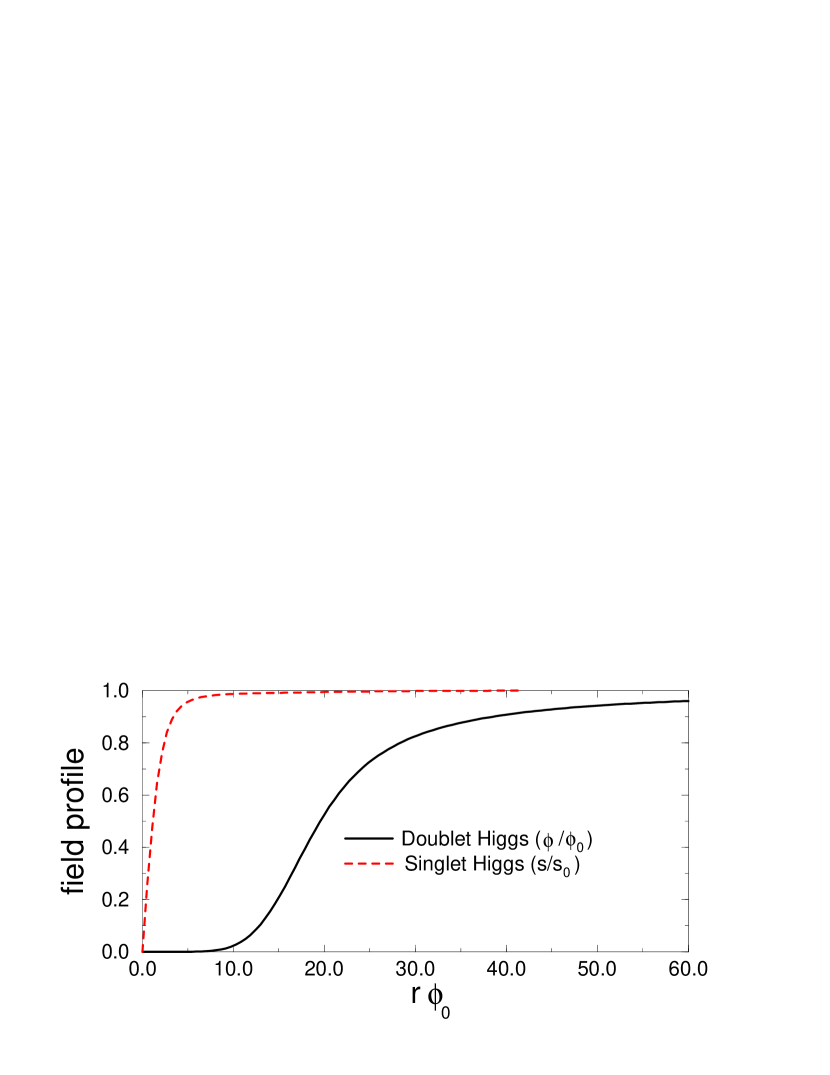
Figure 2: Doublet and singlet Higgs field profiles around a string, for the parameters $\lambda=0.35$, $\lambda_{s}=8.8\times 10^{-5}$, $\gamma=9.4\times 10^{-3}$, and $S_{0}=63\phi_{0}$, where $\Phi_{0}=174$ GeV. These parameters do not allow thermal symmetry restoration of the $S$ field.

the region of symmetry restoration is very wide compared to the weak scale $\Phi_{0}^{-1}\cong 10^{-3}$ fm. In this example, the half-width $r_{1/2}$, where the Higgs field reaches a value of $(\Phi(0)+\Phi_{0})/2$, is nearly 20 times $\Phi_{0}^{-1}$. To get such a wide $\Phi(r)$ profile, it is essential that we use global rather than gauged strings. No radial field excitation in the broken phase is light, and if the $S_{0}$ field approached its asymptotic value exponentially, the region of symmetry restoration could not be wider than the largest inverse mass.

Figure 3 shows how $\Phi(0)$, $r_{1/2}$ and $\hat{m}_{h}^{2}$ depend on $x$ and $y$ for the choices $\hat{\gamma}=1.7$ (same as in figure 2) and $z=1$. The crucial observations are that $\Phi(0)$ tends rapidly toward zero (maximum symmetry restoration in the string) as $S_{0}/\Phi_{0}$ gets large, and the Higgs mass increases most rapidly along the direction of increasing $x\sim y$, while the half-width varies relatively slowly. To increase $r_{1/2}$ dramatically, as in figure 2, one should go to large values of $\hat{m}_{h}^{2}$ and $x\sim y$, and then rescale all the couplings by $z=0.2/\hat{m}_{h}^{2}$, so as to decrease the Higgs mass to the point of saturating the experimental bound. This increases $r_{1/2}$ by the factor $z^{-1/2}$ without changing $\Phi(0)$.

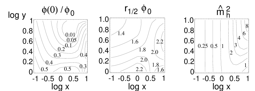
Figure 3: (a,b) Dependence of the Higgs field central value and half-width, $\phi(0)$, $r_{1/2}$ respectively, on the potential parameters $x=\sqrt{\lambda/\lambda_{s}}$ and $y=S_{0}/\Phi_{0}$, for $\hat{\gamma}=1.7$ and $z=1$. The logarithm is base 10. (c) Contours of the dimensionless Higgs mass $\hat{m}_{h}^{2}=m_{h}^{2}/\Phi_{0}^{2}$ for the same parameters.

However we have not yet taken into account the symmetry restoration bound, Eq. (18), which does not allow one to make $\lambda_{s}$ much smaller than $\gamma$. If we saturate this bound, we find that $\hat{\gamma}=2/x$, forcing us to give up at least one of the two baryogenesis-favoring conditions, either that $\hat{\gamma}\sim 2$ or $x\gg 1$. If we give up the latter condition, so that $x\sim 1$ and $\log x\sim 0$, figure 3 shows that $m_{h}$ does not grow with $y$, giving no leverage to rescale $z$ and hence to widen the Higgs field profile. Indeed, eq. (15) shows that in the fixed-$x$, large-$y$ limit, $\hat{m}_{h}^{2}=xz(2-\hat{\gamma}^{2})$. Thus the smallest we can make $z$ is $0.2/(2-\hat{\gamma}^{2})$, which is of order unity or greater if $\hat{\gamma}$ is close to 2. The region of symmetry restoration is of order the weak scale in this case, which is too small to comfortably contain a sphaleron. In fact, the large-$y$, $x\sim 1$ case gives the thin strings we have already considered above. And if we choose $x\sim 1$ and $y\sim 1$, then $\Phi(0)$ is not close to zero; the Higgs field does not lose its condensate even in the core of the string.

If, on the other hand, we try to keep $x$ large while decreasing $\gamma$, the electroweak symmetry restoring effects of the string rapidly diminish, as shown in figure 4, which is the same as figure 3 but for the smaller coupling $\hat{\gamma}=0.1$. As the figure shows, it takes a very large value of $y$ ($S_{0}$) to suppress $\Phi(0)$ in this case; however $r_{1/2}$ decreases with $y$ for fixed $x$, while $m^{2}_{h}$ reaches an asymptotic value. Taking for instance $x=20$, the largest value allowed by the symmetry restoration bound at this value of $\gamma$, we get a string of radius $r_{1/2}<3.5/\phi_{0}$ and $\phi(0)=0.1\phi_{0}$ when $y=100$. Both quantities decrease monotonically with $y$, which must be large in order to suppress the Higgs field in the string core, but the radius over which it is suppressed shrinks at large $y$. For this value, $x=20$, $y=100$, and $\gamma=2\lambda_{s}$, we find a sphaleron energy $0.492$ times the broken phase value. The string cuts the sphaleron energy in half, so the sphaleron rate will be substantially faster than the broken phase rate, but still much slower than the symmetric phase rate, because of the Boltzmann suppression factor $e^{-E_{\rm sph}/T}$. The situation does not improve if we vary $y$ in either direction.

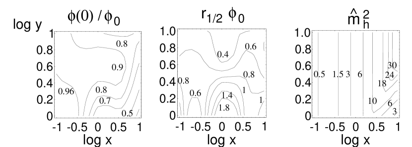
Figure 4: Same as figure 3 but with $\hat{\gamma}=0.1$

It is possible to contrive to evade the symmetry restoration bound, eq. (18). One could add another scalar field $f$ with a positive quartic coupling $\gamma^{\prime}|f|^{2}S^{*}S$, whose sole purpose is to increase the thermal mass of the $S$ field. The constraint is then relaxed to $\gamma<2\lambda_{s}+\gamma^{\prime}$ if $f$ is complex and $\gamma<2\lambda_{s}+\gamma^{\prime}/2$ if $f$ is real. But adding $f$ introduces new problems: $\lambda_{s}$ receives radiative corrections of order $(\gamma^{\prime})^{2}$, which requires fine-tuning of the ultraviolet couplings to preserve the hierarchy $\lambda_{s}\ll|\gamma|$. Furthermore we must either tune $m_{f}<1$ KeV, or give the $f$ particles a direct decay channel by adding a cubic term of form $f|\Phi|^{2}$ and making $m_{f}>4m_{b}$; otherwise they leave an excess relic abundance which overcloses the universe.

It appears possible, then, to allow for “fat” strings with large regions of symmetry restoration, but it requires a highly-tuned hierarchy of couplings in a very artificial model. Aside from this possibility, “fat” global strings do not appear to provide an effective means of restoring electroweak symmetry in a suitably large string core to allow efficient baryon number violation.

To conclude this section, there are two nonsuperconducting string models which allow significant baryon number violation along strings. The case where an extra $U(1)^{\prime}$ is broken by a complex scalar works if the SM Higgs field has a charge $q_{\phi}$ under the $U(1)^{\prime}$ which is incommensurate with the charge $q_{s}$ of the scalar responsible for breaking the $U(1)^{\prime}$ symmetry. The baryon number violation along such a string is much faster than in the broken phase, but is not completely unsuppressed. It is also possible to violate baryon number efficiently in a global string model if the coupling between scalar and Higgs is negative and if there is a large hierarchy of scales between the Higgs self-coupling, the Higgs-singlet coupling, and the singlet self-coupling. However it is also necessary to add a real scalar with cubic couplings and to tune them in a way which is unstable to radiative corrections; thus the model appears to be rather unnatural.

3 Generation of CP asymmetry inside the string

As we saw at the beginning of the last section, the baryon number production is proportional to the product of the sphaleron rate along the string and a CP-odd sum of particle chemical potentials, averaged over the volume in which the sphalerons occur along the string. So besides the sphaleron rate, discussed in the last section, we also need to know how the string biases particle populations, so as to create an asymmetry between particles and their CP conjugates inside the string.

Chemical equilibrium together with CPT ensures that CP-odd combinations of chemical potentials must vanish, so the string only generates such particle distributions if it drives the plasma out of equilibrium, which occurs if the string is moving relative to the plasma. The main goal of this section is to show that, if the string moves slowly, any CP violating chemical potential it generates depends quadratically on the string velocity $v_{s}$. The fact that it goes as $v_{s}^{2}$ and not $v_{s}$ is easy to understand; a string has no natural “front” and “back” sides, so there is no distinction between it moving forward or backward; hence the chemical potentials averaged over the string volume must be even functions of $v_{s}$. Assuming only that the chemical potential on the string has analytic behavior in $v_{s}$, we get that $\mu\sim v_{s}^{2}$ for small $v_{s}$. It remains to check whether this picture is really right, and to see how big the coefficient is.

We will treat this problem in three different ways. First, we will consider an unrealistic model where all parameters are pushed to the extreme values that give the most favorable outcome for baryogenesis. This will be used in the following sections to make a robust argument against the viability of string-mediated baryogenesis. We will then make more realistic estimates of the CP-violating chemical potentials, $\mu_{CP}$, using a purely quantum mechanical treatment for the particle-string interaction, as well as a semiclassical one. It will be seen that both of these give smaller predictions for the size of the CP violating effects than does the toy model. A crucial aspect of these results is the dependence of $\mu_{CP}$ on $v_{s}$, the string velocity. In particular, for small $v_{s}$ we will show that $\mu_{CP}\propto v_{s}^{2}$.

3.1 Model-independent upper limit on ${\mathbf{\mu}_{CP}}$

CP violation at the string wall comes about when the probability for particles to reflect from the wall differs from that of antiparticles. The most extreme situation imaginable for maximizing this effect would occur if the string walls totally reflect particles, and perfectly transmit the corresponding antiparticles. We will make this radical assumption now, in order to get a robust upper limit on $\mu_{CP}$, hereafter simply denoted by $\mu$. Let us now consider how this affects the particle distributions inside the string, where baryon number violation can occur. Since the antiparticles do not see the wall, they are continually refreshed by the equilibrated population outside of the string, so their distribution functions remain thermal. We thus have

$$f_{-}={1\over e^{E/T}\pm 1}=f_{f}\,,$$ (21)

where $f_{f}$ denotes the equilibrium Fermi population function.

The particles, on the other hand, have in addition the effects of the reflections, which in the rest frame of the plasma causes their distribution functions to be boosted by the string velocity (taken to be in the $x$ direction). It is also possible that they acquire a chemical potential, but other departures from equilibrium are damped by collisions. Assuming only that collisions with plasma particles are less frequent than collisions with the walls of the symmetry restored region, which is reasonable for the relatively narrow strings considered in this paper, we get

$$f_{+}={1\over e^{\gamma_{v}(E-v_{s}p_{x}+\mu)/T}\pm 1};\qquad\gamma_{v}=(1-v_{s}^{2})^{-1/2}\,.$$ (22)

For definiteness we will henceforth assume the particles are fermions, and denote them by $F$, since only fermions enter in the anomaly equation and bias baryon number violating processes.

The generation of the chemical potential $\mu$ is due to annihilation ($F\bar{F}\to GG$) and pair-production processes, ($GG\to F\bar{F}$), involving gauge bosons $G$, for example. The size of the equilibrium value of $\mu$ which is generated can be deduced from the Boltzmann equations for the $F$ and $\bar{F}$ distributions: it is that value of $\mu$ which causes the production rate of particles via $GG\to F\bar{F}$ and the destruction rate from $F\bar{F}\to GG$ to cancel each other. This is the right condition because particles inside the string can never get out; if the production and destruction rates did not balance, the particle number would adjust until it did. Let $f_{b}=(e^{E/T}-1)^{-1}$ denote the thermal distribution functions for the gauge bosons, ${\cal M}$ the matrix element for annihilation or pair production, and $d\Pi\equiv\delta(p_{1}+p_{2}-p_{3}-p_{4})\prod_{i=1}^{4}d^{\,3}p_{i}/(16\pi^{3}E_{i})$ the phase space measure. The condition that the collision term vanishes is

$$\int d\Pi|{\cal M}|^{2}\left[f_{+}(p_{1})f_{-}(p_{2})(1+f_{b}(p_{3}))(1+f_{b}(p_{4}))\right.$$

$$\left.-f_{b}(p_{3})f_{b}(p_{3})(1-f_{+}(p_{1}))(1-f_{-}(p_{2}))\right]=0.$$ (23)

Expanding $f_{\pm}$ in powers of $\mu$ and $v_{s}$, and using that $E_{1}+E_{2}=E_{3}+E_{4}$, we find after menial algebra that the term in brackets involving population functions is

$$\left[f_{f}(p_{1})f_{f}(p_{2})(1+f_{b}(p_{3}))(1+f_{b}(p_{4}))\right]\left(\frac{\mu}{T}+v_{s}\frac{p_{1z}}{T}-\frac{v_{s}^{2}}{2}\frac{E^{2}}{T^{2}}+\frac{v_{s}^{2}}{2}\frac{p_{1z}^{2}}{T^{2}}(1-2f_{f}(p_{1}))\right)\,,$$ (24)

plus corrections of order $\mu^{2}$, $v_{s}^{3}$, or $\mu v_{s}$. Since the integration measure contains an average over angles, $p_{z}$ averages to zero and $p_{z}^{2}$ averages to $(1/3)p^{2}$. It is because $p_{z}$ averages to zero that no $v_{s}$ term appears in the expression for $\mu$. It is also clear that for all higher order processes, the term proportional to $v_{s}$ will involve an integration over a vector quantity and will vanish on angular integration; so the $v_{s}^{2}$ dependence of $\mu$ is not an accident of expanding to leading parametric order.

Now, defining

$$\langle X\rangle_{\scriptscriptstyle\cal M}\equiv{\int d\Pi|{\cal M}|^{2}f_{f}(p_{1})f_{f}(p_{2})(1+f_{b}(p_{3}))(1+f_{b}(p_{4}))X\over\int d\Pi|{\cal M}|^{2}f_{f}(p_{1})f_{f}(p_{2})(1+f_{b}(p_{3}))(1+f_{b}(p_{4}))},$$ (25)

then the result for the chemical potential can be simply expressed as

$$\mu={v_{s}^{2}\over 2}\left(\langle E_{2}\rangle_{\scriptscriptstyle\cal M}-{1\over 3T}\left\langle|\vec{p}_{2}|^{2}{e^{E_{2}/T}-1\over e^{E_{2}/T}+1}\right\rangle_{\!\!\scriptscriptstyle\cal M}\right)$$ (26)

Notice that the result is independent of the overall strength of the interaction, ${\cal M}$. This will be true so long as the interaction is faster than the Hubble expansion rate, so that it remains in equilibrium. The answer does involve the energy dependence of ${\cal M}$, but the fact that $\mu\propto v_{s}^{2}$ does not.

To give a concrete estimate for the size of $\mu$, we can simplify the integral by considering the leading logarithmic behavior in the gauge coupling constant $g$, which comes from $t$-channel exchange at low momentum transfer, where ${\cal M}\sim 1/t$. Using the same approximations as in Appendix A of ref. [27], we obtain

$$\mu={\zeta(3)\over 6\zeta(2)}v_{s}^{2}T\cong 0.12v_{s}^{2}T,\qquad v_{s}\ll 1,$$ (27)

in the small-velocity limit. The value of $\mu$, relevant to baryogenesis, is the sum of $1/2$ this quantity, over all left handed doublets coupled to SU(2) which scatter from the wall in this way.

While we have only performed the calculation in the small $v_{s}$ case, where it is valid to make an expansion about equilibrium population functions, we expect that, for relativistic strings,

$$\mu\mathrel{\hbox to0.0pt{\lower 4.0pt\hbox{\hskip 1.0pt$\sim$}\hss}\raise 1.0pt\hbox{$<$}}T,\qquad\gamma_{v}v_{s}\sim 1\,.$$ (28)

since parametrically there is nothing that can enhance $\mu$ to the point of getting a highly degenerate gas of CP-asymmetric particles. In fact, it will be seen that the arguments to be made below would not be invalidated even if $\mu$ diverged like $\gamma_{v}$ in the ultrarelativistic limit.

Eqs. (27-28) are sufficient for making our estimate of the maximum string-mediated baryon asymmetry possible, as will be done below in section 4. To bolster and complete the argument, however, we shall give some more realistic computations of the CP asymmetry in the following subsections.

3.2 Initial chiral flux in a realistic model

We will now consider the generation of a CP-violating particle flux in a specific theory. The simplest example is a two-Higgs-doublet model including [28] a complex mass term $m_{\phi}^{2}\Phi_{1}^{\dagger}\Phi_{2}$ and quartic interaction $h(\Phi_{1}^{\dagger}\Phi_{2})^{2}$. The unremovable CP-violating phase $\theta_{0}$ is defined by $m_{\phi}^{2}h^{1/2}=|m_{\phi}^{2}h^{1/2}|e^{i\theta_{0}}$. In the string wall, the two VEVs can be parameterized as $\Phi_{1}(r)=\phi_{1}(r)e^{i\theta(r)/2}$ and $\Phi_{2}(r)=\phi_{2}(r)e^{-i\theta(r)/2}$, where the $\phi_{i}$ functions are real and $\delta\theta\equiv\theta(\infty)-\theta(0)$ is of order $\theta_{0}$. Solutions for $\theta(r)$ have been found for domain (bubble) wall backgrounds in ref. [28], where $\phi_{i}(r)$ has the form $\tanh(r/r_{0})$, and we expect the solutions to look similar in the case of strings since the shape of our Higgs doublet profiles are qualitatively the same. We will therefore borrow results from ref. [28] to make the following estimates. This is done to be as quantitative as possible, but our main conclusions will not depend on fine details of this particular model, but rather on parametric dependences that we expect to hold in any model.

If each fermion couples only to one of the two Higgs doublets, as is beneficial for avoiding flavor-changing neutral currents, then they will have CP-violating reflections from the string wall as a result of the spatially varying phase $\theta(r)$. Those particles with the largest Yukawa couplings will be reflected most strongly. For simplicity we will model the string as having a square rather than round cross section, moving through the plasma perpendicularly to one of the sides ($\Box\to x$) with velocity $\vec{v}_{s}=v_{s}\hat{x}$. While this approximation is far from perfect, it can only change the answer by a geometrical factor of order 1. It allows the use of planar wall calculations for the difference in reflection probabilities, which can be adequately parameterized in terms of the fermion momentum perpendicular to the string wall (which we will take to be $p_{x}$) by an exponential,

$$\Delta R(p_{x})\cong A\,\delta\theta\,e^{-p_{x}/\delta_{p}}$$ (29)

(the linear dependence on $\delta\theta$ being correct for $\delta\theta\ll 1$), where $A$ and $\delta_{p}$ depend on the mass $m_{f}$ of the fermion outside the string and the width of the Higgs field profile. The dependence of $\delta_{p}$ was found to be

$${\delta_{p}\over m_{f}}=\left\{\begin{array}[]{ll}-1.1\ln(m_{f}r_{1/2})-0.54,&m_{f}r_{1/2}<0.3;\\ 0.19\,(m_{f}r_{1/2})^{-1.2},&0.3<m_{f}r_{1/2}<0.7;\\ 0.15\,(m_{f}r_{1/2})^{-1.8},&m_{f}r_{1/2}>0.7;\end{array}\right.$$ (30)

It should be noticed that, although large values of $r_{1/2}$ are desirable for enhancing the rate of sphaleron interactions in the string, they at the same time suppress the quantum reflections of heavy particles. For this reason lighter particles like the $\tau$ lepton can be more important than top quarks despite their smaller Yukawa couplings.

The amplitude of the asymmetry, $A$, depends not only on $m_{f}r_{1/2}$ but also on $m_{\phi}^{2}/m_{h}^{2}$. For $m_{f}r_{1/2}\sim 1$, $A$ is also of order $0.1$, but for larger $m_{f}r_{1/2}$ it decreases exponentially, $A\cong e^{-cmr_{1/2}}$, where $c$ ranges from $0.5$ to $2$ as $m_{\phi}^{2}/m_{h}^{2}$ goes from 0.3 to 8.

Once $\Delta R$ is known, the next step is to compute the flux of CP asymmetry going into the string. The flux of CP current per unit length of the string is given by

$$J={1\over 2}\int{d^{2}p_{\scriptscriptstyle\perp}dp_{x}\over(2\pi)^{3}}\left|{p_{x}\over E}\right|\Delta R(p_{x})\Bigl{(}f(\gamma_{v}(E+v_{s}\sqrt{p_{x}^{2}-m_{f}^{2}})/T)-f(\gamma_{v}(E-v_{s}p_{x})/T)\Bigr{)},$$ (31)

where $f$ is the distribution function of the particles, boosted by $\pm v$ (the wall velocity) depending on whether they are approaching from the right or the left, and $\gamma_{v}=(1-v_{s}^{2})^{-1/2}$. Making the Maxwell-Boltzmann approximation for the distribution functions, and ignoring the dependence on $m_{f}$ (since the particles are assumed to be relativistic) we can easily evaluate $J$ to be

$$J=v_{s}\,A\,\delta\theta\,{\delta_{p}^{3}\over\pi^{2}}\,{1+\gamma_{v}\delta_{p}/T\over\left(1+2\gamma_{v}\delta_{p}/T+(\delta_{p}/T)^{2}\right)^{2}}$$ (32)

In another theory the form of $J$ might differ, but it must always be proportional to the string velocity, $v_{s}$, because at $v_{s}=0$ everything is in equilibrium. Furthermore, it is bounded by $J\leq v_{s}T^{3}/\pi^{2}$, which is the forward-backwards difference in total incident particle numbers. This bound would be saturated only if the string were a perfect reflector of one CP state and a perfect transmitter of the other; any realistic wall will give currents that are much smaller.

3.3 Subsequent diffusion of the source

Now we are ready to use the current as a source for the diffusion equation to find the steady-state density of chiral asymmetry at the center of the string. It must be understood that the flux $J$ actually represents a positive flux entering the front wall and going into the string, and an equal and opposite flux leaving the string through the front wall and entering the plasma. To apply the diffusion equation, it must be assumed that these fluxes penetrate the plasma by some distance $\lambda$ (the mean free path) before diffusive behavior sets in. Otherwise the diffusion equation sees only two equal and opposite, hence canceling, local densities at the string wall, giving no net source of chiral charge. As explained in references [28, 29], this can be modeled by a source term in the diffusion equation which is a difference of two delta functions:

$${\partial n\over\partial t}-D\left({\partial^{2}\over\partial x^{2}}+{\partial^{2}\over\partial y^{2}}\right)n+\Gamma n=J\left(\delta(x+\lambda-v_{s}t)-\delta(x-\lambda-v_{s}t)\right)$$ (33)

Here $y$ is the transverse direction along the cross-section of the string, $D$ is the fermion’s diffusion constant, and $\Gamma$ is the rate of chirality-damping processes, like spin-flip interactions.

However, the above equation gives only the contribution from the front wall. There is another contribution from the back wall which has the opposite sign. Taking this into account, and changing coordinates to the rest frame of the string, where $x=y=0$ denotes the center, we find that the solution for $n$ can be expressed as a sum of four contributions, two for each wall:

$$n(x,y) = J\Big{[}N(x+w/2+\lambda,y)-N(x+w/2-\lambda,y)$$ (34)

$$\qquad+N(x-w/2+\lambda,y)-N(x-w/2-\lambda,y)\Big{]}\,,$$

where $w=2r_{1/2}$ is the width of the string and $N$ is the Green’s function of the 2-D diffusion equation. The first line represents the front wall contribution and the second is that of the back wall. Although the explicit signs in the equation are the same for both walls, the contributions to the chemical potential at the center of the string are of opposite sign; it is the second and third contributions in the equation which are injected inside of the string. It is only because the string’s motion leads to an asymmetric solution $N$ of the diffusion equation that the expression for $n$ is nonzero at the center of the string; in fact as the string velocity $v_{s}$ goes to zero $N$ becomes a symmetric function and the average over the string interior of the term in brackets goes to zero linearly in $v_{s}$; this is whence the second power of $v_{s}$ arises.

Using the Green’s function for the two-dimensional diffusion equation, the individual contributions are given by

$$N(x,y)={1\over 4\pi D}\int_{0}^{\infty}{dx^{\prime}\over x^{\prime}}\int_{-w/2}^{w/2}dy^{\prime}e^{-(v/4Dx^{\prime})((x+x^{\prime})^{2}+(y-y^{\prime})^{2})-\Gamma x^{\prime}/v},$$ (35)

which satisfies a two-dimensional diffusion equation like (33) with source term

$$\delta(x)\int_{-w/2}^{w/2}dy^{\prime}\delta(y-y^{\prime}).$$ (36)

The derivation of eq. (35) is not completely obvious. For a stationary source, the Green’s function for the 2-D diffusion equation is $G(x,y,t)=t^{-1}\exp(-(x^{2}+y^{2})/4Dt-\Gamma t)$. Now we are considering a moving source, whose trajectory can be described by $x^{\prime}=vt^{\prime}$. At a given position $(x,y)$ and time $t$, an observer sees a contribution from when the source was at position $x^{\prime}$ at the earlier time $t^{\prime}$, proportional to $\int dy^{\prime}G(x-x^{\prime},y-y^{\prime},t-t^{\prime})$. We must integrate all these contributions from $t^{\prime}=-\infty$ to the present time $t$: $N(x,y,t)\propto\int_{-\infty}^{t}dt^{\prime}\int dy^{\prime}G(x-x^{\prime},y-y^{\prime},t-t^{\prime})$. Here $N$ is still in the rest frame of the plasma; replacing $x\to x+vt$ takes us to the rest frame of the source, so that $x$ now measures how far one is in front of the source, and the solution becomes time-independent. The change of variables $x^{\prime}=v(t-t^{\prime})$ in the integral gives eq. (35). As for the normalization, it is chosen to insure that the rate of particle creation by the source equals that of particle loss by decay when the system reaches a steady state:

$$\Gamma\int J\,N(x,y)\,dx\,dy=Jw.$$ (37)

At the center of the string ($y=0$), where the effect is maximized, the answer simplifies somewhat, and can be expressed as

$$N(x)\equiv N(x,0)={e^{-vx/2D}\over 4D\sqrt{\pi}}\int_{0}^{\infty}{dz\over\sqrt{z}}\,{\rm erf}(w/\sqrt{4z})e^{-x^{2}/z-(v/4D)(v/4D+\Gamma/v)z}.$$ (38)

Substituting this result into eq. (34) and evaluating it as a function of $x$, we find that the chiral density in the string is almost antisymmetric about the core, but is skewed slightly by the nonzero velocity, which distinguishes front from back. This behavior (and the fact that we have idealized the string by four delta function sources, eq. (34)) is shown in figure 5. Because $n(x)$ varies significantly inside the core of the string, and the rate of baryon number violation at position $x$ is proportional to $n(x)$, we should average it over the core, i.e., the region $x\in[-w/2,w/2]$:

$$\bar{n}={1\over w}\int_{-w/2}^{w/2}n(x,0)\,dx.$$ (39)

We should also average over $y$, but $n$ is a smooth function of $y$, peaking at $y=0$, so using $y=0$ only slightly overestimates the average. This approximation, in any case, errs in favor of the mechanism we are ruling out.

Figure 5: The chiral asymmetry as a function of distance from the center of the string, for the parameters $D=6/T$, $\lambda=D$, $\Gamma=T/100$, $w=6/T$, $\delta_{p}=0.1T$, and $v=0.1$.

In Figure 6 we show how the spatially averaged chiral asymmetry at the center of the string varies with the string velocity, for several choices of parameters. Set 1: $D=6/T$, $\lambda=D$, $\Gamma=T/100$, $w=6/T$, $\delta_{p}=0.1T$, which is a realistic choice for quarks [30]. Set 2: same as set 1 but with $D=\lambda=100/T$, which might be reasonable for leptons. Set 3: same as set 1 but with $\delta_{p}=T$, to show what happens when the bubble surface efficiently reflects particles with higher momenta. Set 4: same as set 1 but with $w=100/T$, to show what happens for a very thick string. In all examples we have assumed that $T=100$ GeV, which is the temperature where the electroweak phase transition is known to occur, and that CP violation is nearly maximal, $\delta\theta=1$.

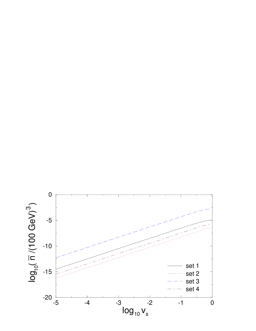
Figure 6: The chiral asymmetry averaged over the string cross section, as a function of the string velocity, treating particle reflections from the string quantum mechanically. See text for description of parameter sets.

In every case the number density, and hence the chemical potential (related by $n=\mu T^{2}/6$ times the number of spin degrees of freedom), varies quadratically with the string velocity, $\mu/T=Kv_{s}^{2}$, with $K$ significantly less than $1$. One power of $v_{s}$ arises from the injected flux, while a second power comes from a front-back cancellation.

To understand why the coefficient of the $v_{s}^{2}$ law is so small, it is important to realize that the string core width is typically not much larger than the quark diffusion constant, and so an asymmetry generated on the string fairly rapidly diffuses away from it into the plasma at large. Since baryon number violation is only efficient right on the string, any chiral asymmetry outside the core is wasted, as far as baryogenesis is concerned, which helps to explain why the coefficient of $\mu$ is so small. Even if we took the flux to be maximal the coefficient $K$ would still be of order $10^{-2}$. This is to be contrasted with the situation in the conventional scenario with a first order phase transition; here the wall is planar, so there is only one direction to diffuse away from it, and baryon number is efficiently violated in one of the half-spaces.

It should be mentioned that the $v_{s}$-dependence of the chemical potential would be different for a very thick string. When the string width satisfies both $r>D/v_{s}$ and $r>T^{3}/\Gamma_{\rm sph}\sim 10^{6}/T$ (where $\Gamma_{\rm sph}\sim 10^{-6}T^{4}$ is the rate per unit volume of sphaleron interactions in the symmetric phase) then the baryon number asymmetry from the front side vanishes; any baryons produced fall into the string and are inevitably destroyed by sphalerons [10]. In this case the baryon number production can scale linearly with $v_{s}$ (although at small enough $v_{s}$, the $r>D/v_{s}$ condition will eventually break down). However, the nonsuperconducting strings we have considered have radii nowhere near this large, and $\mu\propto v_{s}^{2}$ holds up to $v_{s}\sim 1$.

Our treatment becomes less good for $v_{s}$ approaching 1, but we do not expect a large CP asymmetry in this case either. At such large velocities, the flux impinging on the back side of the string can be ignored compared to that which hits the string’s front side and escapes through the back. In the string rest frame, this incident flux is composed of very hard particles. The reflection probability for hard particles drops very quickly with momentum, as was mentioned above, and so therefore does the CP-violating difference in reflection probabilities. In any case, even in a scaling string network where friction is negligible, almost none of the strings are traveling ultrarelativistically; the mean value of $v_{s}^{2}$ (with the average weighted by the energy and not the length of string) is less than 1/2 [32]. For a scaling-regime network what is relevant is an appropriate average of $\mu(v_{s})$ over the velocities represented by the scaling network, for which we expect $\mu\sim T$ with a constant of proportionality roughly of the same order as $K$ the coefficient in the $v^{2}_{s}$ law discussed above.

3.4 WKB estimate of the chiral asymmetry

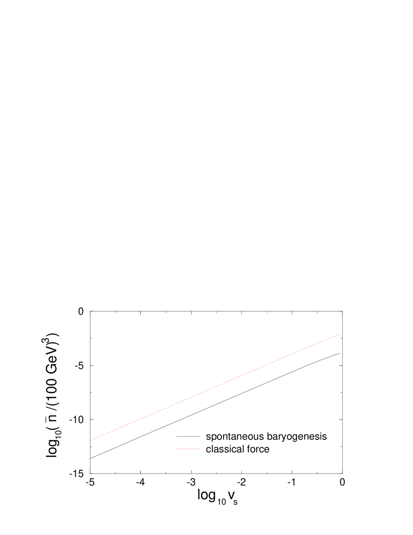
Figure 7: The chiral asymmetry at the center of the string as a function of $v_{s}$, using the WKB approximation, and the parameters $D=6/T$, $\Gamma_{hf}=T/100$, $w=6/T$, $\delta\theta=1$, $y_{f}=1$.

It has been pointed out that when defect boundaries are sufficiently thick compared to the mean free path for particles to scatter in the plasma, a semiclassical treatment of chiral asymmetry generation is more appropriate than the quantum mechanical one given above [30, 31], and gives a larger answer. The distinction arises because CP violation in the defect creates a classical, CP-violating force on particles as they cross the wall. In addition, the scatterings themselves can be CP-violating, giving rise to what has been called “spontaneous baryogenesis” in earlier literature.

If $\theta(x)$ is the background CP-violating phase, such as appears in the two-Higgs-doublet model discussed above, then these two classical effects generically give rise to a source term in the diffusion equation (replacing the r.h.s. of eq. (33)) of the form

$$S(x)\sim v_{s}\,{y_{f}^{2}T^{2}\over 6}\,\left(D\theta^{\prime\prime\prime}+\Gamma_{hf}\theta^{\prime}\right),$$ (40)

where $y_{f}$ is the Yukawa coupling of the fermion to the Higgs field. The primes denote spatial derivatives, and $\Gamma_{hf}$ is the rate of helicity-flipping interactions. The first term is due to the classical force, and the second is the origin of spontaneous baryogenesis. The size of the chemical potential thereby generated can be roughly estimated just as in the previous section if we approximate $\theta$ as a step function, so that $\theta^{\prime}\cong\delta\theta\,\delta(x)$. Taking into account the separate contributions from the front and back walls of the string is accomplished by replacing the above source term by

$$S_{2}(x)=S(x+w/2)-S(x-w/2)$$ (41)

The minus sign occurs because the shape of the $\theta(x)$ profile on the back wall is the mirror image of that on the front wall, and $S(x)$ involves an odd number of derivatives of $\theta(x)$. This behavior is in contrast to the quantum mechanical calculation, where front and back walls gave same-sign contributions. This difference between the quantum and classical treatments stems from the fact that quantum reflection probabilities are the same for particles crossing a potential step, regardless of the direction of motion, whereas the sign of the classical force exerted on the particle by such a step does depend on what direction it is going.

With the delta-function approximation for $\theta^{\prime}$, we can immediately write the spatially averaged solution for the chiral asymmetry in the string, in analogy to the quantum mechanical treatment of the preceding section. $\bar{n}$ is given by eq. (39), using

$$n(x)=v_{s}\,\delta\theta\,{y_{f}^{2}T^{2}\over 6}\left.\left(DN^{\prime\prime}(x^{\prime})+{\Gamma_{hf}}N(x^{\prime})\right)\right|^{x^{\prime}=x+w/2}_{x^{\prime}=x-w/2},$$ (42)

and the definition of $N(x)$ given by eq. (38). The results for the previously-described parameter set 1 ($D=6/T$, $\Gamma_{hf}=T/100$, $w=6/T$, $\delta\theta=1$), assuming $y_{f}=1$, are shown in figure 7. The two terms, due to the spontaneous baryogenesis and classical force effects, respectively, are shown separately. The classical force contribution is larger than the spontaneous baryogenesis contribution, and is also significantly larger than the quantum mechanical prediction for the same set of parameters. The $v_{s}^{2}$ dependence is evident over most of the range of velocities. To convert from density to chemical potential, one uses

$$\mu={6n\over gT^{2}}$$ (43)

for a fermion with $g$ helicity states.

4 Efficiency of baryogenesis by a string network

We have now seen how efficiently baryon number is violated along cosmic strings. Namely, the production of baryons per unit length of string is

$$\frac{dN_{B}}{dLdt}=1.5\kappa_{l}\alpha_{W}^{2}T^{2}\sum_{i}\frac{-\mu_{i}}{T}\,,$$ (44)

where the $\mu_{i}$ are the chemical potentials for the $i$th species of left-handed (SU(2) doublet) fermions. Henceforth we will write $\sum_{i}\mu_{i}$ simply as $\mu$. We have already seen that $\kappa_{l}<0.1$, falling fairly rapidly as the temperature drops, and that $\mu$ varies as $v_{s}^{2}$, the square of the string velocity, when $v_{s}$ is small. To estimate the baryon number produced, we still need to know the density and velocity of the string network, however. These quantities depend crucially on one model-dependent parameter of the strings, namely their tension.

Let us denote the string tension by $\tau$, the typical string’s radius of curvature at the electroweak epoch by $R$, and the typical velocity of propagation of a string, in the rest frame of the plasma, by $v$. On dimensional grounds we have that

$$v\sim HR\,,$$ (45)

with $H$ the Hubble constant at the electroweak epoch.

The string experiences a velocity-dependent friction as it moves through the plasma, arising from particles bouncing off the electroweak-symmetry-restored core of the string. For small velocities one can define a frictional constant $\eta$, such that the force per unit length of string is $d\vec{F}/dL=-\eta\vec{v}$. If $w$ is the width of the symmetry-restored region, then

$$\eta\sim w\eta_{\rm b}\sim\frac{1}{g\phi_{0}}g^{3}\phi_{0}^{3}T\,,$$ (46)

where $\eta_{\rm b}$ is the friction constant of a moving electroweak bubble wall, $\vec{F}/{\rm area}=-\vec{v}\eta_{\rm b}$, and its parametric dependence, $\eta_{\rm b}\sim g^{3}\phi_{0}^{3}T$, was argued in ref. [33]. If we take $\phi_{0}\sim T$, as needed to prevent baryon number violation in the bulk from erasing the baryons produced by strings, then $\eta\sim g^{2}T^{3}$; if instead we make the parametric estimate appropriate right after a weak phase transition, $\phi_{0}\sim gT$, we get $\eta\sim\alpha_{w}^{2}T^{3}$. This is the friction on the string just from its dragging a region of restored electroweak symmetry through the plasma; there may also be additional sources of friction, so the $\eta$ given above is a lower bound.

The force (per unit length) pulling a string forward is given by $\tau/R$. If $v\ll 1$ then inertia is not important and we can equate the forces, and using eq. (45), obtain the estimates

$$\frac{\tau}{R}=v\eta\quad\rightarrow\quad v\sim\sqrt{\frac{H\tau}{\eta}}\,,\,R\sim\sqrt{\frac{\tau}{H\eta}}\,,$$ (47)

valid whenever the resulting velocity is small. This situation is called the friction-dominated regime. On the other hand, if the above estimate gives $v\geq 1$, then friction is not important; instead the string evolution will be dominated by the tension, expansion of the universe, and loss of closed loops due to self-intersections. In this scaling regime, $R\sim 1/H$ and $v\sim 1$, with a mean squared value $\langle v^{2}\rangle<0.5$ [32]. The crossover tension between the two cases for $T\sim 100$ GeV is $\tau\geq(10^{9}{\rm\ GeV})^{2}$.

To obtain the rate of baryon number production per unit volume from eq. (44), we must calculate the total length of string per unit volume. One expects on dimensional grounds that the mean separation between strings is $O(R)$, so the length of string per unit volume is $1/R^{2}$, and the baryon density production rate is

$$\frac{dN_{B}}{dVdt}\sim\left(\frac{1}{R^{2}}\right)\kappa_{l}\alpha_{w}^{2}T^{2}\frac{\mu}{T}\,.$$ (48)

As was discussed in the last section, at small velocities the chemical potential behaves like $\mu=v^{2}KT$, with $K$ a pure number depending on $\phi_{0}/T$ but not on $v$. It was shown that $K$ cannot be larger than $O(1)$, and realistically is much smaller. Similarly, in the large-velocity case, we expect $\mu\leq T$, say, $\mu=K^{\prime}T$.

The two regimes of string evolution can now be considered in turn. First consider the friction-dominated case. Using $\mu=Kv^{2}T$ and eq. (45) in (48) gives

$$\frac{dN_{B}}{dVdt}\sim\kappa_{l}\alpha_{w}^{2}KH^{2}T^{2}\,.$$ (49)

This expression must be integrated from the time when the Higgs condensate first becomes large enough to preserve baryon number in the broken phase, $\phi_{0}\simeq T$, to the present time. The right hand side depends on time through the temperature, $d(\ln T)/dt\sim H$. The most strongly temperature-dependent term is $\kappa_{l}$, which decreases quickly with falling temperature. Even making the generous assumption that it takes one Hubble time for $\kappa_{l}K$ to fall sufficiently to cut off baryon number production, we still get a final baryon density of order

$$\frac{N_{B}}{VT^{3}}\sim\kappa_{l}K\alpha_{w}^{2}\frac{H}{T}\sim\kappa_{l}K\alpha_{w}^{2}\frac{T}{m_{\rm pl}}\,.$$ (50)

The last step follows from the Friedmann equation, $H^{2}=(8\pi/3)(\rho/m_{\rm pl}^{2})$, using $\rho\sim T^{4}$, so $H\sim T^{2}/m_{\rm pl}$. In this expression, all dependence on the density of the string network, i.e., on $1/R$, has dropped out. This happens because, although a denser network of strings produces baryons along a greater total length of string, these strings are moving more slowly and are therefore less efficient at baryon number production.

The above argument neglects the effects of small closed loops of string, yet the string velocity in a friction-dominated network can become large for a loop just as it collapses. One may wonder whether such loops can enhance the baryon production. To answer this, consider a loop initially of radius $r=R$, the characteristic curvature length of the network, which subsequently shrinks. Its velocity is $v(r)\propto 1/r$, and the radius evolves as $dr/dt=-v$. Hence $r\propto(t_{0}-t)^{1/2}$, with $t_{0}$ the time of final collapse. The baryon production is proportional to

$$\int^{t_{0}}Lv^{2}dt=2\pi\int^{t_{0}}rv^{2}dt\propto\int^{t_{0}}(t_{0}-t)^{-1/2}dt\,,$$ (51)

which is well-behaved at the upper limit of integration and dominated by $r\sim R$. Hence the collapse of loops contributes approximately as much to the baryon asymmetry as the evolution of the rest of the network, parametrically no more.

Putting in the most optimistic values, $\kappa_{l}\sim 10^{-1}$, $K\sim 10^{-2}$, $T/m_{\rm pl}\sim 10^{-17}$, we find a baryon asymmetry about 13 orders of magnitude smaller than the physical value, $N_{B}/(VT^{3})\sim N_{B}/N_{\gamma}\sim 10^{-10}$.

If the string network is in the scaling regime, the previous argument changes as follows. Rather than $\mu=Kv^{2}T$, with $K\leq 1$, we have $\mu=K^{\prime}T$ with $K^{\prime}\leq 1$. Also, $R\sim 1/H$ rather than $R\sim v/H$. The final expression is the same with $K^{\prime}$ substituted for $K$, and the generated baryon number is still too small by at least 13 orders of magnitude.

These estimates are optimistic, in the sense that $\kappa_{l}$ falls quite quickly with temperature, so there is much less than one Hubble time for baryon number to be created; moreover $K$ is realistically much less than $10^{-2}$. The treatment of the defect network is somewhat pessimistic, though, since numerical studies show that the mean separation of cosmic strings is closer to $1/10$ of the Hubble length, rather than the full Hubble length [32]. This could enhance our estimate of the baryon asymmetry by a factor of $10^{2}$. Also, the coefficients of order unity in the Friedmann equation imply that $H\sim 10\,T^{2}/m_{\rm pl}$, winning us an additional factor of 10. But this still leaves the mechanism too weak by 10 orders of magnitude, even using the most optimistic assumptions.

Interpretation: Free Energy

There is another way of understanding our result, by considering the available free energy in a network. Think of the out of equilibrium requirement of baryogenesis as the statement that a baryogenesis mechanism must be a way of converting available free energy into baryon number.

The available free energy density in the conventional electroweak baryogenesis scenario, with bubble walls converting supercooled symmetric phase into broken phase, is the free energy difference between the phases, which is $(T_{c}-T_{\rm nuc})\Delta S$, the temperature drop between equilibrium and nucleation times the entropy difference of the phases. The numerical value is parametrically $O(\alpha_{W}^{3}T^{4})$ for $\lambda\sim g^{2}$, but it is always at least $10^{-3}T^{4}$ when the phase transition is strong enough to prevent subsequent erasure of the baryon number.

For the string network, the available free energy is the free energy contained in the network, which is the length of string times the tension (times the mean value of the relativistic $\gamma$ factor for the scaling network, but this is order 1). For the friction dominated network, the density of the network is $\sim 1/R^{2}$, which together with Eq. (47) gives a free energy density $\sim H\eta\mathrel{\hbox to0.0pt{\lower 4.0pt\hbox{\hskip 1.0pt$\sim$}\hss}\raise 1.0pt\hbox{$<$}}T^{4}(T/m_{\rm pl})$, independent of the tension. Since the baryogenesis mechanism is the same or similar as that in the conventional first order case, it would be surprising if this much smaller available store of free energy were able to produce anything like the same number of baryons. For the scaling network the available free energy is larger, though observational constraints require it to be less than $10^{-6}T^{4}$. However, most of the free energy loss is not due to friction against the plasma. In fact, the amount which is being lost to heating the plasma directly is independent of the tension of the network, since the width of the symmetry restored region does not depend on the string width. In fact the free energy loss to the plasma is about $\eta$ times the area swept out by the network in a Hubble time, $\sim H\eta$, which is parametrically the same as for the friction dominated network. In either case, the network is just not capable of generating anywhere near the amount of departure from equilibrium needed to produce enough baryons.

The situation might be different for a superconducting network, but the above reasoning suggests that even for this case, baryogenesis can only get close to the efficiency of the conventional first order mechanism if the free energy of the network is close to the observational limit and much or most of the network’s energy is lost to the plasma.

5 Conclusion

String networks do not provide a viable scenario for electroweak baryogenesis if the strings are not superconducting. While they are capable of generating baryons, they do so far too inefficiently to account for the existing abundance.

The first problem is that baryon number violation along a string, while certainly faster than in the broken phase, is not entirely unsuppressed. The core where electroweak symmetry is restored is never wide enough to allow symmetric phase sphaleron-like events; at best it brings the sphaleron rate to $1/30$ of what it would be in the unsuppressed case, i.e., if the core region was $1/\alpha_{w}T$ in diameter.

Given the actual width of the region of symmetry restoration around a cosmic string, we find that if the network is in the scaling regime, it violates baryon number in far too small a total volume for it to add up to the observed abundance. If the network evolution is friction-dominated, the network is denser, but the denser is the network, the more slowly moving the strings are. This in turn makes them very inefficient at creating baryon number, since the production rate goes as $v^{2}$ for small velocity. In either case the generated baryon number is at least 10 orders of magnitude smaller than the observed abundance.

The case of superconducting cosmic strings merits more careful study. The main challenge here is finding a realistic estimate of the hypercharge current carried by a typical string at the electroweak epoch. We have not attempted to study this problem here. However, our results make it clear that unless the region of symmetry restoration proves to be much wider than $1/g^{2}T$, the superconducting scenario will also fail.

Appendix A Cooling to a saddle point

Here we discuss an algorithm for numerically finding a saddle point of a Hamiltonian on a many-dimensional space, which we used for determining the energy for a sphaleron in a string background in Section 2.

Suppose that we have a Hamiltonian system with degrees of freedom $\Phi_{\alpha}$ and Hamiltonian $H(\Phi)$. We require only that the coordinates $\Phi$ are continuous. They could for instance be real numbers, or members of a compact manifold.

Ordinary gradient flow cooling of the fields means evolving the fields under a cooling time $\tau$ according to

$$\frac{d\Phi_{\alpha}}{d\tau}=-\frac{\partial H(\Phi(\tau))}{\partial\Phi_{\alpha}}\,.$$ (52)

When the $\Phi$ take values on a manifold the derivatives are understood in terms of the tangent space at the current location. A typical discrete implementation of this algorithm is

$$\Phi_{\alpha}(\tau+\Delta)-\Phi_{\alpha}(\tau)=-\Delta\frac{\partial H(\Phi(\tau))}{\partial\Phi_{\alpha}}\,.$$ (53)

When $\Phi$ is a point on a manifold, the right hand side is a point in the tangent space of $\Phi(\tau)$ and we determine $\Phi(\tau+\Delta)$ by starting at $\Phi(\tau)$ and following the geodesic curve of starting direction and length indicated by the right hand side.

Provided that we make $\Delta$ small enough, this algorithm will reduce the energy until it hits a local minimum. “Small enough” means that $\Delta<2/\omega^{2}_{\rm max}$, where $\omega^{2}_{\max}$ is the largest eigenvalue of the matrix of second derivatives of $H$. In many cases we can actually compute, or at least bound, $\omega^{2}_{\rm max}$ over the entire space, and ensure stable dissipation.

What if we want an algorithm which will flow to the nearest extremum, even if it is a saddle point and not a minimum? If we can guess a starting point which is fairly close to the desired extremum then it makes sense to analyze algorithm behavior in terms of small deviations about the extremum. Write the fields as $\Phi_{0}+\delta\Phi_{\alpha}$, and expand the Hamiltonian to second order in $\delta\Phi_{\alpha}$;

$$H\simeq H(\Phi_{0})+H_{\alpha\beta}\delta\Phi_{\alpha}\delta\Phi_{\beta}\,.$$ (54)

The matrix $H_{\alpha\beta}$ is diagonalized by the basis of eigenvectors $\xi_{\alpha}$, with eigenvalues $\lambda_{\alpha}$. It is convenient to write the distance from the extremum $\Phi_{0}$ in this basis, as $\delta_{\alpha}\xi_{\alpha}$.

The action of the algorithm, Eq. (53), on $\delta_{\alpha}$ is

$$\delta_{\alpha}(\tau+\Delta)=[1-\Delta\lambda_{\alpha}]\delta_{\alpha}(\tau)\,,$$ (55)

which shrinks those perturbations in directions with positive eigenvalue and stretches perturbations in directions with negative eigenvalue. This is fine if you want to find a minimum but it will carry you away from a saddle point.

If on the other hand we take $N$ steps with step length $\Delta$ and one step with step length $-N\Delta$, the departure from the saddle point is

$$\delta_{\alpha}({\rm after})=[1+N\Delta\lambda_{\alpha}][1-\Delta\lambda_{\alpha}]^{N}\delta_{\alpha}({\rm before})\simeq(1+N\Delta\lambda_{\alpha})e^{-N\Delta\lambda_{\alpha}}\delta_{\alpha}({\rm before})\,,$$ (56)

where the last approximation holds for $\Delta\lambda\ll 1$. We plot the function $(1+x)e^{-x}$ in Figure 8. The

Figure 8: The function $(1+x)e^{-x}$. The algorithm converges for all eigenvalues $\lambda$ provided $N\Delta\lambda\equiv x$ satisfies $-1<(1+x)e^{-x}<1$.

algorithm reduces the deviation in every basis direction provided that the most negative eigenvalue $\lambda_{\rm neg}$ satisfies $1+N\Delta\lambda_{\rm neg}e^{-N\Delta\lambda_{\rm neg}}>-1$, which requires $N\Delta\lambda_{\rm neg}>-1.2784645$. If we choose $N\Delta$ too large, the deviation in the unstable direction will alternate in sign and grow in magnitude; otherwise every departure from the saddle point will shrink.

For our application we can tell if we have chosen too large a value for $N\Delta$ by cooling the configuration towards vacuum and finding the sign of ${\rm Tr}E\cdot B$ as the configuration slides out of the saddle towards the vacuum. If $N\Delta\lambda_{\rm neg}<-1$ then the sign of the excitation in the unstable direction switches each step, and so will the direction of approach towards the vacuum. If the sign switches we may be driving the system dangerously. If it does not, we are being too conservative and the algorithm will be inefficient. We can adjust $N\Delta$ as we go to achieve optimal stable performance. If we did not have such a clear signature for the sign of the unstable mode, we could still determine $\lambda_{\rm neg}$, once we get close to the saddle point, by tracking the energy during cooling from near the saddle to the vacuum. After transients from stable modes have decayed, but before the configuration gets far from the saddle, the energy behaves like $E_{\rm sph}-K\exp(\tau\lambda_{\rm neg})$, and $\lambda_{\rm neg}$ can be determined by fitting.

Also note that, if we know $\lambda_{\rm neg}$, and also know that there is only one unstable mode, we can increase the efficiency with which the algorithm eliminates low frequency stable modes by applying extra cooling. For instance we can perform a backwards step of length $1/\lambda_{\rm neg}$ and several small forward steps of total length $2/|\lambda_{\rm neg}|$, so the departure from the saddle point obeys

$$\delta_{\alpha}({\rm after})=(1+\lambda_{\alpha}/\lambda_{\rm neg})\exp(-2\lambda_{\alpha}/\lambda_{\rm neg})\delta_{\alpha}({\rm before})\,.$$ (57)

However, if we expect there to be more than one negative eigenmode then this is may make the other one grow unstably. In general, if there are more than 1 negative eigenmodes and there are low lying positive eigenmodes, the algorithm becomes quite inefficient. Also note that the algorithm will not necessarily find a saddle point if it starts out very far from it. Both of these limitations are quite general limitations of saddle point finding algorithms. The algorithm’s charm is its simplicity; all we need to be able to do is take first derivatives of the Hamiltonian in order to apply it, though we should try to determine $\lambda_{\rm neg}$ if we want to apply it well. No more coding is necessary than it takes already to search for minima.

References

- [1] For recent reviews see G. Steigman, astro-ph/9803055; K. Olive, astro-ph/9712160.
- [2] E.W. Kolb and M.S. Turner, Ann. Rev. Nucl. Part. Sci. 33, 645 (1983).
- [3] V.A. Rubakov and M.E. Shaposhnikov, Usp. Fiz. Nauk 166, 493 (1996), Phys. Usp. 39, 461 (1996).
- [4] For reviews see for instance A.G. Cohen, D.B. Kaplan and A.E. Nelson, Annu. Rev. Nucl. Part. Sci. 43, 27 (1993); A.D. Dolgov, Phys. Rept. 222, 309 (1992); A. Riotto, hep-ph/9807454.
- [5] A.D. Sakharov, Zh. Eksp. Teor. Fiz. Pis’ma 5, 32 (1967); JETP Lett. 91B, 24 (1967).
- [6] G. ’t Hooft, Phys. Rev. Lett. 37, 37 (1976); Phys. Rev. D14, 3432 (1976).
- [7] V.A. Kuzmin, V.A. Rubakov and M.E. Shaposhnikov, Phys. Lett. B155, 36 (1985).
- [8] See for instance B. de Carlos and J. R. Espinosa, Nucl. Phys. B 503, 24 (1997); M. Carena, M. Quirós, and C.E.M. Wagner, Nucl. Phys. B 524, 3 (1998); D. Bödeker, P. John, M. Laine and M.G. Schmidt, Nucl. Phys. B497, 387 (1997); J. Cline and G. D. Moore, hep-ph/9806354, to appear in Phys. Rev. Lett. (1998); M. Losada, hep-ph/9806519; M. Laine and K. Rummukainen, hep-lat/9804019; hep-ph/9804255, Phys. Rev. Lett.
- [9] M. Trodden, A. Davis and R. Brandenberger, Phys. Lett. B335 (1994) 123, Phys. Lett. B349 (1995) 131; M. Trodden, hep-ph/9803479.
- [10] R. Brandenberger, A. Davis, T. Prokopec and M. Trodden, Phys. Rev. D53 (1996) 4257.
- [11] For a comprehensive review see M. Hindmarsh and T. Kibble, Rept. Prog. Phys. 58, 477 (1995).
- [12] W. Perkins and A.C. Davis, Nucl. Phys. B406, 377 (1993).
- [13] P. Bock et al., CERN-EP-98-046.
- [14] M. García-Pérez and P. van Baal, Nucl. Phys. B 429, 451 (1994).
- [15] G. D. Moore and N. Turok, Phys. Rev. D 56, 6533 (1997).
- [16] P. Arnold, D. Son, and L. Yaffe, Phys. Rev. D 55, 6264 (1997).
- [17] P. Huet and D. Son, Phys. Lett. B393, 94 (1997).
- [18] D. Son, UW/PT-97-19, hep-ph/9707351.
- [19] G. D. Moore, C. Hu, and B. Müller, Phys. Rev. D 58, 045001 (1998).
- [20] D. Bödeker, Phys. Lett. B 426, 351 (1998).
- [21] F. Klinkhamer and N. Manton, Phys. Rev. D 30, 2212 (1984).
- [22] L. Yaffe, Phys. Rev. D 40, 3463 (1989); J. Kunz and Y. Brihaye, Phys. Lett. B 216, 353 (1989).
- [23] G. D. Moore, MCGILL-98/7, hep-ph/9805264.
- [24] L. Carson and L. McLerran, Phys. Rev. D 41 (1990) 647; L. Carson, X. Li, L. McLerran, and R. Wang, Phys. Rev. D 42, 2127 (1990).
- [25] G. D. Moore, Nucl. Phys. B 493, 439 (1997); Nucl. Phys. B 523, 569 (1998).
- [26] J. Ambjørn and A. Krasnitz, Phys. Lett. B 362, 97 (1995).
- [27] G. D. Moore and T. Prokopec, Phys. Rev. D 52, 7182 (1995).
- [28] J. Cline, K. Kainulainen, and A. Vischer, Phys. Rev. D 54, 2451-2472 (1996).
- [29] M. Joyce, T. Prokopec, and N. Turok, Phys. Rev. D 53, 2930 (1996).
- [30] M. Joyce, T. Prokopec, and N. Turok, Phys. Rev. D 53, 2958 (1996).
- [31] J. Cline, M. Joyce, and K. Kainulainen, hep-ph/9708393, Phys. Lett. B 417, 79 (1998).
- [32] D. Bennett and F. Bouchet, Nuffield Workshop 1989, pg 321; Phys. Rev. D 41, 2408 (1990).
- [33] G. D. Moore and N. Turok, Phys. Rev. D 55, 6538 (1997).