Soft dilepton production and hard thermal loops

Abstract

The Hard Thermal Loop expansion, is an attractive theory, but it reveals difficulties when one uses it as a perturbative scheme. To illustrate this we use the HTL expansion to calculate the two loop corrections for soft virtual photons. The resulting corrections are of the same order as the 1-loop correction.

LAPTH-98/702, hep-ph/9810246

I Introduction

The production of soft photons (energy $\sim gT$, where $g\ll 1$ is the strong coupling constant) in a hot quark-gluon plasma at equilibrium has been studied by many groups, using thermal field theory [1, 2, 3, 4, 5], or a semi-classical approach as in [6, 7, 8]. In this talk I will study the case of soft virtual photon (with invariant mass $Q^{2}\sim g^{2}T^{2}$) at two-loop level using the Hard Thermal Loop (HTL) expansion. The two loop diagrams are found to be of the same order of magnitude as the one loop result. This unexpected result solves the problem of the absence of bremsstrahlung in the HTL expansion, while bremsstrahlung seems to contribute dominantly when using the semi-classical approach [6, 7, 8].

II Motivations and problems

The starting point will be the bare thermal field theory. The imaginary part of the photon polarization which is proportional to the invariant dilepton production rate is found to be:

$${\rm Im}\Pi^{\mu}_{\mu} \sim e^{2}Q^{2}(1-2n_{F}(\frac{Q}{2}))$$ (1)

$$\sim e^{2}g^{3}T^{2}\qquad{\rm for}\quad q,q_{o}\sim gT\;.$$ (2)

The additional power of $g$ in ${\rm Im}\Pi^{\mu}_{\mu}$ arises from the fact that the soft photon is produced by annihilation of a soft quark-antiquark pair (each of momentum $Q/2$). Other processes such as $q\rightarrow\gamma q$ are not allowed since the quark is massless. Having a soft momentum scale, the HTL expansion [9, 10, 11, 12] demands the use of effective vertices and propagators. The soft virtual photon production was one of the first applications of the HTL resummation scheme [3]: the authors of [3] have calculated the imaginary part of the one loop diagram of Fig. 1. In Fig. 1 we have depicted some of the cuts that give relevant physical amplitudes. Cuts [a] and [b] of the one loop diagram in Fig. 1 can be approximated by :

$${\rm Im}\,\Pi^{\mu}{}_{\mu}(Q)_{|{\bf[a,b]}}\sim e^{2}g^{3}{{T^{2}}}\int\limits_{{gT}}^{{T}}\frac{dp}{p}\;,$$ (3)

where p is the quark momentum in the loop, where we have used explicitly $q_{o}\sim gT$.

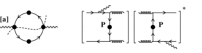
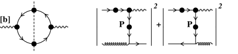
FIG. 1.: 1-loop contribution to the soft photon production and some of the different cuts responsible for different physical processes; in [b] one of the two fermion momenta is space like while the other is time like.

A few remarks are worth saying about this result:
$\bullet$ The HTL is built to handle soft momentum problems; in the hard momentum limit, it tells that we recover the bare theory which is a priori what one needs in most cases. For example if we take a fermion with momentum $P$, the inverse of its effective propagator is given by the sum of the inverse bare propagator ($/$$P$) and the one-loop correction as shown in Fig. 2: to evaluate this correction one should apply the HTL approximation. Thus in the one-loop correction in Fig. 2 we use $L+P\approx L$, which is justified if $P$ is soft and the loop momentum $L$ is hard, but when $P$ becomes hard this approximation is no more correct, then the HTL estimate of the one-loop correction of the effective propagator is incomplete in the hard momentum limit.

FIG. 2.: The inverse of the fermion effective propagator.

$\bullet$ The processes shown in Fig. 1 come from one loop corrections to the bare vertices and propagators. On the other hand the integral $\int\limits_{gT}^{T}\frac{dp}{p}\sim\ln(1/g)$ in Eq. 3, indicates that the quark momentum runs from a soft scale ($gT$) to a hard scale ($T$), i.e. we need the hard limit of the one loop correction which is incomplete in the HTL approximation as we mentioned before.
$\bullet$ The importance of processes coming from cut [a] in Fig 1 can be understood from the result of Cleymans et al [6, 7, 8], where they calculated bremsstrahlung photon production (Fig. 3) using a semi classical approach: their result yields ${\rm Im}\,\Pi^{\mu}{}_{\mu}(Q)\sim e^{2}g^{3}T^{2}$ which is of the same order as Eq. 2 and Eq. 3.

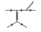
FIG. 3.: Bremsstrahlung photon production.

$\bullet$ The bremsstrahlung photon production (Fig. 3) is mediated by the gluon exchange, while that of cut [a] of Fig. 1 is mediated by the exchange of quark, and it is reasonable to think that a complete calculation should include both processes. The natural question that arises is: how can one reconcile bremsstrahlung with the HTL scheme?

III 2-loop diagrams

The solution to the problems mentioned in Sect. II comes when one looks at 2-loop diagrams in the HTL expansion. In two loop diagrams we have more powers of $g$, coming from the $qqg$ vertices, then to compensate additional powers of $g$ which may come from the phase space we have to have a hard phase space. In the catalogue of 2-loop diagrams we skip those which contain vertices with no bare analogue: these vertices turn out to be negligible when one of the vertex lines becomes hard. The remaining diagrams are shown in Fig. 4. As discussed in F. Gelis’s talk [15], calculating two loop diagrams in the HTL expansion , one should pay attention to the counterterms in order to avoid double-counting (see also [16] for more details.).

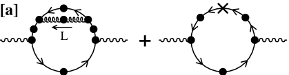
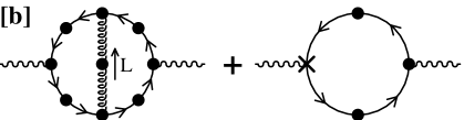
FIG. 4.: Two-loop contributions involving bremsstrahlung processes. A black dot denotes an effective propagator or vertex. Crosses are HTL counterterms.

We explore the case where all the quark momenta are hard. Assuming hard quark momentum we can replace the effective vertices by the bare ones, and take the bare propagator for the quark. The simplified version of Fig. 4 is represented in Fig. 5. In the same figure we have depicted the relevant cuts that enable one to calculate the corresponding contribution in the framework of the thermal cutting rules.

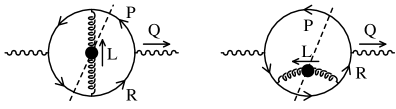
FIG. 5.: Simplified two-loop contributions involving bremsstrahlung processes.

In what follows we will take the photon to be static i.e. $Q^{\mu}=(q_{o},{\mathchoice{{\hbox{\boldmath$\displaystyle 0$}}}{{\hbox{\boldmath$\textstyle 0$}}}{{\hbox{\boldmath$\scriptstyle 0$}}}{{\hbox{\boldmath$\scriptscriptstyle 0$}}}})$. For virtual photon the production rate per unit time and per unit volume is related to the imaginary part of the retarded polarization tensor of the photon as [17, 18]:

$${{dN}\over{dtd{\mathchoice{{\hbox{\boldmath$\displaystyle x$}}}{{\hbox{\boldmath$\textstyle x$}}}{{\hbox{\boldmath$\scriptstyle x$}}}{{\hbox{\boldmath$\scriptscriptstyle x$}}}}}}=-{{dq_{o}d{\mathchoice{{\hbox{\boldmath$\displaystyle q$}}}{{\hbox{\boldmath$\textstyle q$}}}{{\hbox{\boldmath$\scriptstyle q$}}}{{\hbox{\boldmath$\scriptscriptstyle q$}}}}}\over{12\pi^{4}}}\;{\alpha\over{Q^{2}}}\,n_{{}_{B}}(q_{o})\,{\rm Im}\,\Pi^{{}^{R}}{}_{\mu}{}^{\mu}(q_{o},{\mathchoice{{\hbox{\boldmath$\displaystyle q$}}}{{\hbox{\boldmath$\textstyle q$}}}{{\hbox{\boldmath$\scriptstyle q$}}}{{\hbox{\boldmath$\scriptscriptstyle q$}}}})\;.$$ (4)

The gluon propagator appears linearly in ${\rm Im}\,\Pi_{\mu}{}^{\mu}$, then we can write:

$${\rm Im}\,\Pi_{\mu}{}^{\mu}\sim{\rm Im}\,\Pi_{\mu}{}^{\mu}\left|{}_{{L^{2}<0}}+{\rm Im}\,\Pi_{\mu}{}^{\mu}\left|{}_{{L^{2}>0}}\right.\right.\;,$$ (5)

where $L$ is the momentum flow through the gluon.
Such separation is motivated by the fact that regions $L^{2}<0$ and $L^{2}>0$ contain different physical processes. While $L^{2}<0$ gives bremsstrahlung of Fig. 3, which is a possible candidate to reconcile bremsstrahlung with the HTL expansion, $L^{2}>0$ gives annihilation and Compton scattering. Bremsstrahlung is a new process, then we can guarantee that it will give a positive contribution that should be added to the one-loop result. Moreover we can apply different approximations in each of these regions. We can treat each region separately and at the end we add the two contributions. In the next sections we will discuss in detail the region $L^{2}<0$, while we will give some indicative results for $L^{2}>0$.

IV Bremsstrahlung

The matrix element ${\cal M}$ of diagrams [a] and [b] of Fig. 5 , can be written as (see [16] for the complete expression):

$${\cal M}\sim{\cal M}_{1}L^{2}+{\cal M}_{2}\;.$$ (6)

Writing ${\cal M}$ in this form exhibits some of the terms that are absent at one loop level in the HTL expansion. Indeed the gluon appearing in the effective propagator and vertices in the one loop diagram are taken to be light-like ($L^{2}=0$) by construction of the HTL resummation scheme, then ${\cal M}_{1}$ will be a pure 2-loop contribution.

A Extraction of logarithmic behavior

We can obtain analytically the leading logarithmic behavior in $\ln(1/g)$ of ${\rm Im}\,\Pi_{\mu}{}^{\mu}$ at 2-loop order. By momentum power counting we can isolate the term which gives the logarithm: it happens that this term comes from ${\cal M}_{1}$, enforcing the previous expectation that bremsstrahlung contribution is a pure two loop contribution.
The contribution of this leading term can be written schematically as:

$${\rm Im}\,\Pi^{{}^{R}}{}_{\mu}{}^{\mu}(q_{o},{\mathchoice{{\hbox{\boldmath$\displaystyle 0$}}}{{\hbox{\boldmath$\textstyle 0$}}}{{\hbox{\boldmath$\scriptstyle 0$}}}{{\hbox{\boldmath$\scriptscriptstyle 0$}}}})\approx{\rm A}\times e^{2}g^{2}\left(\frac{1}{q_{o}}\right)m^{2}_{\rm g}\int\limits_{0}^{T}dp\int\limits_{f(m_{\rm g},q_{o})}^{T}\frac{dl}{l}\;.$$ (7)

Comments:
$\bullet$ A is a constant that depends on the color factors, and it has no $g$ dependence.
$\bullet$ $e^{2}$ comes from the $qq\gamma$ couplings.
$\bullet$ $g^{2}$ comes from the $qqg$ couplings.
$\bullet$ $\frac{1}{q_{o}}$ comes from the uncut quark-propagator denominators, for example the momentum $R$ in Fig. 5 can be approximated by: $R^{2}=2q_{o}p$.
$\bullet$ The soft gluon thermal mass $m_{\rm g}^{2}\equiv g^{2}T^{2}[N+N_{{}_{F}}/2]/9$, comes from the gluon spectral density.
$\bullet$ The ultraviolet cutoff $T$ is provided by the statistical weights.
$\bullet$ The integral $\int\limits_{0}^{T}dp$ indicates the hard $p$ behavior.
$\bullet$ $f(m_{\rm g},q_{o})$ is a function of dimension one. This function depends on both $q_{o}$ which appears as a kinematical infrared cut-off in the integral over $dl$ and $m^{2}_{\rm g}$ which appears in the gluon spectral density and can also play the role of an infrared cut-off for the same integral.
$\bullet$ The integral $\int\limits_{f(m_{\rm g},q_{o})}^{T}\frac{dl}{l}$ points out that $l$ vary between a soft scale ($f\sim gT$) and a hard scale ($T$).
The cutoff $f$ can be simplified by taking $q_{o}\ll m_{\rm g}\sim gT\ll T$, then the larger cutoff $m_{\rm g}$ will be the relevant cutoff. After this simplification we get:

$${\rm Im}\,\Pi^{{}^{R}}{}_{\mu}{}^{\mu}(q_{o},{\mathchoice{{\hbox{\boldmath$\displaystyle 0$}}}{{\hbox{\boldmath$\textstyle 0$}}}{{\hbox{\boldmath$\scriptstyle 0$}}}{{\hbox{\boldmath$\scriptscriptstyle 0$}}}})\approx-{{3NC_{{}_{F}}e^{2}g^{2}}\over{8\pi^{3}}}{{m^{2}_{\rm g}T}\over{q_{o}}}\ln\left({{T^{2}}\over{m^{2}_{\rm g}}}\right)\;.$$ (8)

The production rate is then given by:

$$\left.{{dN}\over{dtd{\mathchoice{{\hbox{\boldmath$\displaystyle x$}}}{{\hbox{\boldmath$\textstyle x$}}}{{\hbox{\boldmath$\scriptstyle x$}}}{{\hbox{\boldmath$\scriptscriptstyle x$}}}}}}\right|_{\rm bremss}\approx{{dq_{o}d{\mathchoice{{\hbox{\boldmath$\displaystyle q$}}}{{\hbox{\boldmath$\textstyle q$}}}{{\hbox{\boldmath$\scriptstyle q$}}}{{\hbox{\boldmath$\scriptscriptstyle q$}}}}}\over{8\pi^{6}}}NC_{{}_{F}}\alpha^{2}\Big{(}\sum_{f}e^{2}_{f}\Big{)}\left({{m_{\rm g}\over{q_{o}}}}\right)^{2}$$ (9)

$$\times\left({{gT}\over{q_{o}}}\right)^{2}\ln\left({{T^{2}}\over{m^{2}_{\rm g}}}\right)\;,$$ (10)

where the sum runs over the flavor of the quarks in the loop ($e_{f}$ is the electric charge of the quark of flavor $f$, in units of the electron electric charge).
Numerical estimates of the unapproximated expression of ${\rm Im}\,\Pi_{\mu}{}^{\mu}$ verify that the condition $q_{o}\ll m_{\rm g}$ is only a technical condition as we get a reasonable accuracy even for $q_{o}/m_{\rm g}\sim 10$. On the other hand $m_{\rm g}/T$ must be smaller than 0.1 in order to have an agreement between the approximate and the complete expression with an accuracy better than 5 % (see Fig. 6).

 

FIG. 6.: Comparison of numerical estimates of the complete matrix element with the simple theoretical expression obtained in Eq. (10). Both plots show the ratio “Numerical/Theoretical”. On the left plot, $q_{o}/T$ is fixed at $10^{-4}$ and we look at the variations with $m_{\rm g}/T$ (i.e.  with $g$). On the right plot, $m_{\rm g}/T$ is fixed at $10^{-2}$ and the photon energy varies from ultra-soft energies to hard ones.

B Comparison with other approaches

1 Braaten et al. results

The production rate of soft static photons has been evaluated by Braaten, Pisarski and Yuan in [3] at one-loop in the HTL scheme. To compare Eq. 10 with the result of [3] in the domain $q_{o}\ll m_{\rm g}\sim gT\ll T$ for which our expression is justified, one has to isolate from their result the processes which have the same nature and spectrum (in $\frac{1}{q_{o}^{4}}$) as the bremsstrahlung, i.e those of Fig. 1-[a]. Applying the same approximation we did in Sect. IV A, we can easily extract the $\ln(1/g)$ in BPY’s result:

$$\left.{{dN}\over{dtd{\mathchoice{{\hbox{\boldmath$\displaystyle x$}}}{{\hbox{\boldmath$\textstyle x$}}}{{\hbox{\boldmath$\scriptstyle x$}}}{{\hbox{\boldmath$\scriptscriptstyle x$}}}}}}\right|_{\rm 1-loop}\!\!\!\!\!\approx{{dq_{o}d{\mathchoice{{\hbox{\boldmath$\displaystyle q$}}}{{\hbox{\boldmath$\textstyle q$}}}{{\hbox{\boldmath$\scriptstyle q$}}}{{\hbox{\boldmath$\scriptscriptstyle q$}}}}}\over{12\pi^{4}}}N\alpha^{2}\Big{(}\sum_{f}e^{2}_{f}\Big{)}\left({{m_{{}_{F}}\over{q_{o}}}}\right)^{4}\ln\left({{T^{2}}\over{m^{2}_{{}_{F}}}}\right)\;,$$ (11)

where $m^{2}_{{}_{F}}=g^{2}C_{{}_{F}}T^{2}/8$ is the soft quark thermal mass.
Comments:

• The production rate in Eq. 11 and Eq. 10 have the same spectrum in $\frac{1}{q_{o}^{4}}$.

• $m^{2}_{{}_{F}}$ plays the role of an infrared regulator in Eq. 11, while $m_{\rm g}$ is the regulator in Eq. 10. This reflects the different nature of both results, an exchanged fermion in the first, and an exchanged gluon in the second.

• Comparing the two results we obtain the ratio:

  $${{\left.{{dN}}\right|_{\rm bremss}}\over{\left.{{dN}}\right|_{\rm 1-loop}}}\approx{{32}\over{3\pi^{2}}}{{N+N_{{}_{F}}/2}\over{C_{{}_{F}}}}\;,$$ (12)

  which for 2 light flavors and 3 colors becomes

  $${{\left.{{dN}}\right|_{\rm bremss}}\over{\left.{{dN}}\right|_{\rm 1-loop}}}\approx{{32}\over{\pi^{2}}}\sim 3.2\;.$$ (13)

  This ratio is rather large, which means that bremsstrahlung is definitely an essential contribution to the soft static photon production rate by a hot plasma.

2 Cleymans et al. results

We return to the semi-classical treatment used in [6, 7, 8]. In their approach they took into account the effect of multiple scattering of the quark in the plasma. To compare the two loop result with their result one need to “undo” the effect of rescattering and consider only one collision of the quark in the plasma. We apply the same simplification as they did i.e.:

• The scattering of the particles is treated as in vacuum (the dynamics), while the plasma effects are introduced for the kinematics only.

• The energy of the quarks or gluons is much larger than the temperature so that Boltzman distributions are used for particles entering the interaction region and a factor 1 is assigned to those leaving it. As a by-product one can neglect the photon momentum compared to the momenta of the constituents in the plasma.

• To screen the forward singularity they introduced a phenomenological Debye mass $m_{{}_{D}}$, which we will take to be $m_{\rm g}$ when we compare their result with Eq. 10.

Applying the above approximations we get for the production rate of the lepton pair at rest the following expression:

$${{{dN}\over{dtd{\mathchoice{{\hbox{\boldmath$\displaystyle x$}}}{{\hbox{\boldmath$\textstyle x$}}}{{\hbox{\boldmath$\scriptstyle x$}}}{{\hbox{\boldmath$\scriptscriptstyle x$}}}}}}}\approx{dq_{o}d{\mathchoice{{\hbox{\boldmath$\displaystyle q$}}}{{\hbox{\boldmath$\textstyle q$}}}{{\hbox{\boldmath$\scriptstyle q$}}}{{\hbox{\boldmath$\scriptscriptstyle q$}}}}\over{3\pi^{6}}}{\alpha^{2}\alpha_{s}^{2}}{d_{f}d}\Big{(}\sum_{f}e^{2}_{f}\Big{)}{T^{4}\over q_{o}^{4}}\ln\left({{T^{2}}\over{m^{2}_{{}_{D}}}}\right)\;,$$ (14)

where $d_{f}=2_{s}\times 3_{c}=6$ and $d=\frac{4}{9}\ 2\times 2_{f}\times 2_{s}\times 3_{c}+2_{s}\times 8_{c}=26+{2\over 3}$ are the degeneneracy factors introduced in [7].
From Eq. 14 we see that the semi-classical approach give the same spectrum in $\frac{1}{q_{o}^{4}}$ as expected.
Comparing with Eq. 10 we find for two flavors:

$${\left.{dN}\right|_{\rm semi-class}\over\left.{dN}\right|_{\rm bremss}}\approx{15\over\pi^{2}}\;,$$ (15)

i.e. the semi-classical over-estimates the rate of production by about $50\%$. This difference appears to come from the various approximations they used .

V Preliminary results for time like gluon

In this section we give partial results for the $L^{2}>0$ case [19] and the arguments that we will give are based on the leading logarithmic behavior only.
The basic physical processes for $L^{2}>0$ are Compton and annihilation, then naively we expect double counting with the one loop diagram, in the region where the imaginary part of the one loop diagram gives similar processes (Fig. 1-[b]). To cure this problem of double counting , we have to calculate the counterterms depicted on the right of Fig. 4. Indeed, when the gluon in the loop becomes hard, we have a hard loop that reproduce what is already included in the one-loop diagram via the effective vertices and propagators .
The structure of ${\rm Im}\,\Pi_{\mu}{}^{\mu}$ allows to decompose it as the sum of two pieces, one part reflecting the hard gluon momentum behavior (${\rm Im}\,\Pi_{1}$) where we can apply the hard $L$ approximation, and the other reflecting the hard fermion behavior (${\rm Im}\,\Pi_{2}$):

$${\rm Im}\,\Pi\simeq{\rm Im}\,\Pi_{1}+{\rm Im}\,\Pi_{2}\;.$$ (16)

A Hard $L$ region

By isolating hard $L$ terms we apply indirectly the HTL approximation, then one may expect a fair compensation between ${\rm Im}\,\Pi_{1}$ and the counterterms. ${\rm Im}\,\Pi_{1}$ reveals soft $p$ sensitivity, which means that it is no more allowed to use the bare propagator for the quark, thus we have to use the effective one. At leading logarithm order we can take a constant mass for the quark which will be the asymptotic quark thermal mass which is twice the soft quark thermal mass $m_{{}_{F}}$. This mass will play along with $q_{0}$ the role of an infrared regulator.
Then the contribution of ${\rm Im}\,\Pi_{1}$ to the production rate is approximated by:

$$\left.\frac{dN}{d^{4}xdq_{o}d^{3}{\mathchoice{{\hbox{\boldmath$\displaystyle q$}}}{{\hbox{\boldmath$\textstyle q$}}}{{\hbox{\boldmath$\scriptstyle q$}}}{{\hbox{\boldmath$\scriptscriptstyle q$}}}}}\right|^{{\rm Im}_{1}}\approx\frac{N\sum_{f}e_{f}^{2}}{12\pi^{4}}\frac{\alpha^{2}m_{f}^{2}}{q_{o}^{2}}\ln\left(\frac{T}{g(m_{{}_{F}},q_{o})}\right)\;,$$ (17)

where $g$ is a function of $m_{f}$ and $q_{o}$. To evaluate the imaginary part of the counter term diagrams (CT) we follow [3], where the authors relate the imaginary part of the effective vertex to the spectral density function. Then the imaginary part of the counter term diagrams may be expressed in terms of the spectral density of the quark propagator. After a cumbersome calculation, the logarithmic behavior of the counter terms can be estimated by:

$$\left.\frac{dN}{d^{4}xdq_{o}d^{3}{\mathchoice{{\hbox{\boldmath$\displaystyle q$}}}{{\hbox{\boldmath$\textstyle q$}}}{{\hbox{\boldmath$\scriptstyle q$}}}{{\hbox{\boldmath$\scriptscriptstyle q$}}}}}\right|^{\rm CT}\approx-\frac{N\sum_{f}e_{f}^{2}}{12\pi^{4}}\frac{\alpha^{2}m_{{}_{F}}^{2}}{q_{o}^{2}}\ln\left(\frac{2Tq_{o}}{h(m_{{}_{F}},q_{o})}\right)\;,$$ (18)

where $h$ is a function of $m_{{F}}$ and $q_{o}$.
The only difference between Eq. 17 and Eq. 18 is that they have different infrared regulator, adding both Eqs. we get a logarithm of argument of ${\cal O}(1)$, which remains finite, even in the limit of vanishing thermal masses , then we can neglect the total contributions coming from ${\rm Im}\,\Pi_{1}$ and the counterterms compared to $\ln(1/g)$ that we will get from ${\rm Im}_{2}$ .

B Hard $p$ region

In the hard $p$ limit we are lead to the same type of analysis as for $L^{2}<0$ where there is no need for the effective propagator, thus we use the bare propagator for the quark. The different behavior of the spectral density for $L^{2}<0$ and $L^{2}>0$ leads to different behavior of the terms in the matrix element, for example the term that gives the leading logarithm in ${\rm Im}\;\Pi_{2}$ comes from ${\cal M}_{2}$ in Eq. 6. Different behavior will lead to different spectrum in each case.
Taking a constant thermal mass for the gluon, we can obtain analytically the leading logarithmic behavior of ${\rm Im}_{2}$:

$${\rm Im}\;\Pi_{2}(q_{o},{\mathchoice{{\hbox{\boldmath$\displaystyle 0$}}}{{\hbox{\boldmath$\textstyle 0$}}}{{\hbox{\boldmath$\scriptstyle 0$}}}{{\hbox{\boldmath$\scriptscriptstyle 0$}}}})\approx{{NC_{{}_{F}}e^{2}g^{2}}\over{4\pi^{3}}}{q_{o}}T\ln\left(\frac{T}{m_{\rm g}\left(\frac{m_{\rm g}}{q_{o}}+\frac{q_{o}}{m_{\rm g}}\right)}\right)\;.$$ (19)

The production rate is then given by:

$$\left.\frac{dN}{d^{4}xdq_{o}d^{3}{\mathchoice{{\hbox{\boldmath$\displaystyle q$}}}{{\hbox{\boldmath$\textstyle q$}}}{{\hbox{\boldmath$\scriptstyle q$}}}{{\hbox{\boldmath$\scriptscriptstyle q$}}}}}\right|^{{\rm hard\;\;}p}\!\!\approx\!\!\frac{2N\sum e_{f}^{2}}{3\pi^{6}}\frac{\alpha^{2}m_{{}_{F}}^{2}}{q_{o}^{2}}\ln\left(\frac{T}{m_{\rm g}\left(\frac{m_{\rm g}}{q_{o}}+\frac{q_{o}}{m_{\rm g}}\right)}\right)\;,$$ (20)

which has a $\frac{1}{q_{o}^{2}}$ spectrum compared to the $\frac{1}{q_{o}^{4}}$ of bremsstrahlung.

C Comparison with Braaten et al. result

To compare Eq. 20 with the one loop result obtained in [3], we consider only the kinematical region which gives rise to processes shown in Fig. 1-[b], i.e. the region where one of the quarks in the loop is space like while the other is time like. Applying the same approximation done to obtain Eq. 19 we get for the diagram [b] of Fig. 1:

$$\left.\frac{dN}{d^{4}xdq_{o}d^{3}{\mathchoice{{\hbox{\boldmath$\displaystyle q$}}}{{\hbox{\boldmath$\textstyle q$}}}{{\hbox{\boldmath$\scriptstyle q$}}}{{\hbox{\boldmath$\scriptscriptstyle q$}}}}}\right|^{\rm 1loop}\approx\frac{N\sum e_{f}^{2}}{12\pi^{4}}\frac{\alpha^{2}m_{{}_{F}}^{2}}{q_{o}^{2}}\ln\left(\frac{2Tq_{o}}{{\rm Max}(q_{o}^{2},m_{{}_{F}}^{2})}\right)\;,$$ (21)

which has the same spectrum in $\frac{1}{q_{o}^{2}}$ as the production rate at two loops in Eq. 20. Adding Eqs. 20 and 21 we get for the annhilation and Compton scattering up to two loops:

$$\frac{dN}{d^{4}xdq_{o}d^{3}{\mathchoice{{\hbox{\boldmath$\displaystyle q$}}}{{\hbox{\boldmath$\textstyle q$}}}{{\hbox{\boldmath$\scriptstyle q$}}}{{\hbox{\boldmath$\scriptscriptstyle q$}}}}}\approx\frac{N\sum e_{f}^{2}}{3\pi^{6}}\frac{\alpha^{2}m_{f}^{2}}{q_{o}^{2}}\left\{\frac{\pi^{2}}{4}\ln\left(\frac{2Tq_{o}}{{\rm Max}(q_{o}^{2},m_{F}^{2})}\right)\right.$$ (22)

$$\left.\!\!\!\!\!\!\!\!\!\!\!\!\!+2\ln\left(\frac{T}{m_{\rm g}\left(\frac{m_{\rm g}}{q_{o}}+\frac{q_{o}}{m_{\rm g}}\right)}\right)\right\}\;.$$ (23)

The ratio of the two-loop contribution to the one-loop result is given by:

$${{\left.{{dN}}\right|_{\rm 2-loops}}\over{\left.{{dN}}\right|_{\rm 1-loop}}}\approx{{8}\over{\pi^{2}}}\sim 0.81\;.$$ (24)

This signifies that the two-loop contribution is essential. Being calculated with $p$ taken hard from the beginning, ${\rm Im}\,\Pi_{2}$ will complete the contribution coming from the 1-loop result which assumes $p$ to be soft compared to the momentum of the hard loop in the resumed propagators and vertices. This cures (at least at leading logarithmic behavior) the problem mentioned in Sect. II, that the hard thermal loop does not give the complete estimate of the loop corrections to the effective quantities in the limit of hard momentum. To sum-up, the one-loop diagram takes care of the soft $p$ region, while the two-loop diagrams with the counter terms complements the one loop estimate by taking care of the hard $p$ region.

To verify the above result we take the thermal masses to zero in the logarithms in Eq. 23:

$$\frac{dN}{d^{4}xdq_{o}d^{3}{\mathchoice{{\hbox{\boldmath$\displaystyle q$}}}{{\hbox{\boldmath$\textstyle q$}}}{{\hbox{\boldmath$\scriptstyle q$}}}{{\hbox{\boldmath$\scriptscriptstyle q$}}}}}\approx\frac{N\sum e_{f}^{2}}{3\pi^{6}}\frac{\alpha^{2}g^{2}C_{{}_{F}}}{8q_{o}^{2}}(\frac{\pi^{2}}{4}+2)\ln(T/q_{o})\;.$$ (25)

This coincides with the production rate calculated in [2] at two-loop level using the bare thermal field theory.

VI Further problems

Our result reveals also a logarithmic sensitivity, i.e. the gluon which is supposed to be soft, is extrapolated by the logarithmic behavior ($\int\limits_{gT}^{T}\frac{dl}{l}$) to the hard region, which bring again the problem of the hard limit of the HTL approximation at next to leading order. A complete result may need to include higher order contributions as the 3-loop diagrams of Fig. 7. Probably one has also to consider the other topologies of 3-loop diagrams to have a gauge independent set of diagrams, without forgetting the associated counterterms.

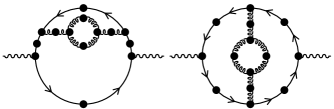
FIG. 7.: A set of 3-loop diagrams that may give a dominant contribution, diagrams where the gluon loop is replaced by a fermion loop is also of the same nature.

The importance multiple scattering of the quark in the plasma (Landau-Pomeranchuk effect) in [6, 7, 8], points again the importance of higher order diagrams.

VII Conclusion

We have discussed the production of virtual soft dilepton production in a hot quark-gluon plasma in thermal equilibrium. This special case may give some indicative properties of the hard thermal loop expansion as a perturbative scheme. We have shown that to get the total contributions at a given order in the coupling constant $g$, one has to add contributions that comes from different loop orders, i.e. increasing the number of loops does not necessarily mean that the result is suppressed by additional powers of $g$. The case of soft virtual photon we considered illustrates that, even in the absence of any divergences, loop-order mixing occurs. Moreover the two-loop diagrams give rise to new physical processes which do not appear at one loop. Using the method of counterterms we give an explicit way to calculate higher loop diagrams using the HTL expansion. There exists other methods in the literature, such as using a cutoff [20, 21, 22, 23] in order to obtain the correct behavior of the effective propagator in the hard momentum limit and to avoid possible double counting.Finally adding the contributions coming from $L^{2}>0$ and $L^{2}<0$ the virtual photon production rate in the plasma is increased considerably which may have remarkable experimental effects.

REFERENCES

-
[1]
R. Baier, B. Pire, D. Schiff, Phys. Rev. D38, 2814 (1988);
T. Altherr, P. Aurenche, T. Becherrawy, Nucl. Phys. B315, 436 (1989);
T. Altherr, T. Becherrawy, Nucl. Phys. B330, 174 (1990);
Y. Gabellini, T. Grandou, D. Poizat, Ann. Phys. 202, 436 (1990). - [2] T. Altherr, P. Aurenche, Z.Phys. C 45, 99 (1990).
- [3] E. Braaten, R.D. Pisarski, T.C. Yuan, Phys. Rev. Lett. 64, 2242 (1990).
- [4] J.Cleymans, I. Dadić , Phys. Rev. D 47, 160 (1993)
- [5] P. Aurenche, F. Gelis, R. Kobes, E. Petitgirard, Z. Phys. C 75, 315 (1997).
- [6] J. Cleymans, V.V. Goloviznin, K. Redlich, Phys. Rev. D 47, 989 (1993).
- [7] J. Cleymans, V.V. Goloviznin, K. Redlich, Z. Phys. C 59, 495 (1993).
- [8] V.V. Goloviznin, K. Redlich, Phys. Lett. B 319, 520 (1993).
- [9] E. Braaten, R.D. Pisarski, Nucl. Phys. B 337, 569 (1990).
- [10] E. Braaten, R.D. Pisarski, Nucl. Phys. B 339, 310 (1990).
- [11] J. Frenkel, J.C. Taylor, Nucl. Phys. B 334, 199 (1990).
- [12] J. Frenkel, J.C. Taylor, Nucl. Phys. B 374, 156 (1992).
- [13] R.L. Kobes, G.W. Semenoff, Nucl. Phys. B 260, 714 (1985).
- [14] R.L. Kobes, G.W. Semenoff, Nucl. Phys. B 272, 329 (1986).
- [15] F. Gelis, these proceedings.
- [16] P. Aurenche, F. Gelis, R. Kobes, H. Zaraket, hep-ph/9804224, to appear in Phys. Rev. D.
- [17] H.A. Weldon, Phys. Rev. D 28, 2007 (1983).
- [18] C. Gale, J.I. Kapusta, Nucl. Phys. B 357, 65 (1991).
- [19] Work in progress.
- [20] E. Braaten, T.C. Yuan Phys. Rev. Lett. 66, 2183 (1991).
- [21] E. Braaten, M. Thoma, Phys. Rev. D44, 1298 (1991)
- [22] R. Baier, H. Nakkagawa, A. Niegawa, K. Redlich, Z. Phys. C 53, 433 (1992).
- [23] J.I. Kapusta, P. Lichard, D. Seibert, Phys. Rev. D 44, 2774 (1991).