KUNS-1534

HE(TH)98/15

hep-ph/9810204

Right-handed neutrino mass and bottom-tau ratio
in strong coupling unification

Masako Bando and Koichi Yoshioka

^∗Aichi University, Aichi 470-02, Japan

^†Department of Physics, Kyoto University Kyoto 606-8502, Japan

The recent results of neutrino experiments indicate the existence of the right-handed neutrinos with masses around intermediate scale, which affects the prediction of the bottom-tau mass ratio. In the minimal supersymmetric standard model, this effect largely depends on the right-handed neutrino mass scale and then may severely limit its lower bound. In this letter, we show that in the case of strong coupling unification the bottom-tau mass ratio is little affected by the presence of the right-handed neutrinos. This is because of the infrared fixed-point behavior of Yukawa couplings, which is a common feature of this kind of model.

The gauge coupling unification is one of the remarkable successes of the minimal supersymmetric standard model (MSSM) [1] and provides us with a strong phenomenological support to the MSSM. The bottom to tau mass ratio, $R$ $(\equiv y_{b}/y_{\tau})$, is another phenomenological support of the MSSM and has been intensively studied [2]. With the $SU(5)$ unification condition of Yukawa couplings, $y_{b}=y_{\tau}$, the $SU(3)_{C}$ gauge coupling effect gives $R(M_{Z})\sim 2.2$, which was almost a desirable low-energy value. However, a more accurate experimental data on the bottom and tau masses [3] gives

$$R(M_{Z})\,\simeq\,1.6-1.8,$$ (1)

which strongly constrains the allowed region of relevant parameter space. In order to reproduce the above ratio, it is known that the top (and/or bottom) Yukawa coupling should be very large so that it suppresses the $SU(3)_{C}$ gauge coupling effect [2].

Now, the recent neutrino experiments strongly indicate the existence of right-handed neutrinos. In particular, the atmospheric neutrino anomaly [4] can be solved by neutrino oscillation scenario between two neutrino species with squared mass difference $\sim 10^{-(2-3)}$ eV². By the seesaw mechanism [5], this fact suggests that the right-handed neutrino mass scale $M_{R}$ is of an intermediate scale. The existence of right-handed neutrinos at an intermediate scale is also favored by cosmology and astrophysics from various points of view (hot dark matter [6], baryogenesis [7], inflation [8], etc.). However, in the MSSM, if the third generation right-handed neutrino exists at such an intermediate scale we have a following 1-loop renormalization group equation (RGE) for $R$ in the region between the GUT scale $M_{G}$ and $M_{R}$:

$$\frac{dR}{dt}\,=\,\frac{R}{16\pi^{2}}\left[(y_{t}^{2}-y_{\nu}^{2})+3(y_{b}^{2}-t_{\tau}^{2})-\left(\frac{16}{3}g_{3}^{2}-\frac{4}{3}g_{1}^{2}\right)\right],$$ (2)

where $g_{i}\,(i=1,2,3)$ are gauge couplings of the standard gauge group $SU(3)_{C}\times SU(2)_{W}\times U(1)_{Y}$, and $t\equiv\ln\mu$. In the above equation, a new ingredient from $y_{\nu}$, which is absent in the usual MSSM, gives an opposite contribution to that of the top Yukawa coupling. If one assumes the $SO(10)$-like boundary condition, $y_{t}=y_{\nu}$, the neutrino Yukawa coupling largely reduces the effect of the top Yukawa coupling and increases the low-energy value of the bottom-tau ratio. This effect of $y_{\nu}$ imposes the strong restriction on the allowed region of $M_{R}$ and/or $\tan\beta$ [9, 10]. In particular, in the small $\tan\beta$ case, the severe constraint for the lower bound of $M_{R}$ is found. If one considers the tau-neutrino as a hot dark matter candidate the lower bound of $M_{R}$ translates into an upper bound on the neutrino hot dark matter density of the universe, which is much smaller than the cosmologically interesting range [10].

So far, there are several ways to avoid this situation. Within the MSSM framework, one way is to modify the right-handed neutrino Majorana mass matrix, in which the mass of the third-generation right-handed neutrino is much larger than the intermediate scale. This can be achieved consistently with the quark-lepton parallelism preserving the large mixing between the second and third generation neutrinos [11]. The GUT scale physics may also change the bottom-tau ratio by modifying the boundary condition, $y_{b}=y_{\tau}$, with relevant Higgs fields [12], by the corrections from GUT scale physics [13, 10], and so on. If one can adopt the models with an intermediate gauge group beyond the standard model [14], the boundary condition, $y_{b}=y_{\tau}$, preserves down to a breaking scale of an intermediate gauge group and the right-handed neutrinos, which get masses of this breaking scale, give no harmful effect on the low-energy bottom-tau ratio.

In this letter, we suggest an alternative approach to this problem in the framework of the standard gauge symmetry. We point out that in strong coupling unification scenario such a bound on $M_{R}$ does not exist in contrast to the MSSM case (weak coupling unification). In the strong coupling unification scenario [15], the gauge couplings behave asymptotically non-freely yielding a strong unified gauge coupling ($\sim O(1)$). For a concrete model, we here take the extended supersymmetric standard model (ESSM) with 5 generations; the MSSM + 1 extra vector-like family [16, 17], as a typical example of the strong coupling unification model. However, the results are not specific to the ESSM but common features in general strong unification models.

In the ESSM, the RGEs of the Yukawa couplings at 1-loop level are as follows:

$$\frac{dy_{t}}{dt} = \frac{y_{t}}{16\pi^{2}}\left(9y_{t}^{2}+y_{b}^{2}+2y_{\nu}^{2}-\frac{16}{3}g_{3}^{2}-3g_{2}^{2}-\frac{13}{15}g_{1}^{2}\right),$$ (3)

$$\frac{dy_{b}}{dt} = \frac{y_{b}}{16\pi^{2}}\left(y_{t}^{2}+9y_{b}^{2}+2y_{\tau}^{2}-\frac{16}{3}g_{3}^{2}-3g_{2}^{2}-\frac{7}{15}g_{1}^{2}\right),$$ (4)

$$\frac{dy_{\tau}}{dt} = \frac{y_{\tau}}{16\pi^{2}}\left(6y_{b}^{2}+5y_{\tau}^{2}+y_{\nu}^{2}-3g_{2}^{2}-\frac{9}{5}g_{1}^{2}\right),$$ (5)

$$\frac{dy_{\nu}}{dt} = \frac{y_{\nu}}{16\pi^{2}}\left(6y_{t}^{2}+y_{\tau}^{2}+5y_{\nu}^{2}-3g_{2}^{2}-\frac{3}{5}g_{1}^{2}\right).$$ (6)

Here, we consider only the 3rd and 4th generation Yukawa couplings and neglect the other generations (throughout this letter, we set the mass of the extra families to be the same order of the SUSY breaking scale $M_{S}$ ($\simeq 1$ TeV) [16, 17]). This assumption correctly reproduces the low-energy top quark mass as its infrared fixed-point value. Up to this level there is no difference between the MSSM and the ESSM in the expression of the RGE for $R$ (eq. (2)). Note that the other generation Yukawa couplings, if included, affects the RGE for $R$ very little since they are very small or come in below 2-loop level.

There are two characteristic features in the ESSM which are important in investigating the behavior of the low-energy bottom-tau ratio. One is that, due to the strong gauge couplings, some of the Yukawa couplings (over gauge coupling) at low-energy scale are determined almost insensitively to their initial values at $M_{G}$ because they reach their infrared fixed points very rapidly [18]. This is physically significant because we can get important information on the physical parameters independently of unknown high-energy physics. The other is the boundary condition of the bottom and tau Yukawa couplings. Generally, one must adopt the unification condition $y_{\tau}>y_{b}$ in such a strong unification model because of the strong enhancement effect on the bottom-tau ratio from $SU(3)_{C}$ gauge interaction. In the ESSM, we impose the boundary condition of the Yukawa couplings as $y_{\tau}=3y_{b}$ at $M_{G}$ by assuming the Higgs field of the $\overline{126}$ ($\overline{45}$) representation of $SO(10)$ ($SU(5)$). With this boundary condition, we showed that the correct observed bottom-tau mass ratio can be reproduced when we do not include the effects of neutrino Yukawa couplings [17].

To see these two points more concretely, it is instructive to use the semi-analytic expression of the low-energy value of $R$. If all the Yukawa couplings are neglected, by formally integrating the 1-loop RGE (eq. (2)), we have

$$\frac{R(M_{Z})}{R(M_{G})} = f_{R}\left(\frac{\alpha_{3}(M_{S})}{\alpha_{3}(M_{G})}\right)^{8/9}\left(\frac{\alpha_{1}(M_{S})}{\alpha_{1}(M_{G})}\right)^{10/99},\qquad{\rm(MSSM)}$$ (7)

$$\frac{R(M_{Z})}{R(M_{G})} = f_{R}\left(\frac{\alpha_{3}(M_{S})}{\alpha_{3}(M_{G})}\right)^{-8/3}\left(\frac{\alpha_{1}(M_{S})}{\alpha_{1}(M_{G})}\right)^{10/159},\qquad{\rm(ESSM)}$$ (8)

where $f_{R}$ is an enhancement factor of $R$ which comes from the net contributions between $M_{S}$ and $M_{Z}$ including the effect of the top Yukawa and $SU(3)_{C}$ gauge couplings ($f_{R}\sim 1.2$). In the MSSM case (7), we have $R(M_{Z})/R(M_{G})\sim 2.4$ for $\alpha_{3}(M_{Z})=0.12$, which is somewhat larger than the present experimental value. On the other hand, in the ESSM case (8), the strong unified gauge coupling considerably enhances $R(M_{Z})$. However, as mentioned above, Yukawa couplings evolve up to their theoretical infrared fixed points very quickly just below the GUT scale in the ESSM. Including the effects of Yukawa couplings as their infrared fixed-point values which are obtained from eq. (3), we have

$$\frac{R(M_{Z})}{R(M_{G})} \simeq f_{R}\left(\frac{\alpha_{3}(M_{S})}{\alpha_{3}(M_{G})}\right)^{-7/5}\left(\frac{\alpha_{1}(M_{S})}{\alpha_{1}(M_{G})}\right)^{10/159}.\qquad{\rm(ESSM)}$$ (9)

This factor gives $R(M_{Z})/R(M_{G})\sim(5-6)$ (for $\alpha_{3}(M_{Z})=0.12$). Therefore, we can get a correct low-energy bottom-tau ratio if we take the boundary condition, $y_{\tau}=3y_{b}$ $(R(M_{G})=1/3)$, which can be naturally obtained from a single relevant Higgs field ($\overline{126}$ ($\overline{45}$) of $SO(10)$ ($SU(5)$)) [12]. Then, it is our task to see how the right-handed neutrinos affect on this successful prediction of the bottom-tau ratio in strong unification models.

With the common expression of the RGE for $R$, however, there are two notable differences in the cancellation effect between Yukawa couplings because of the above mentioned two characteristic features of the ESSM; the infrared fixed-point structure of (top) Yukawa coupling and the boundary condition of the bottom and tau Yukawa couplings. Especially, due to the latter effect, the neutrino Yukawa coupling $y_{\nu}$ decreases more rapidly as $\mu$ decreases from $M_{G}$. This is because the effect of Yukawa couplings is very large because of the boundary condition $y_{\tau}=3y_{b}$ together with their large coefficients in the beta function (6). These two effects on the cancellation between $y_{t}$ and $y_{\nu}$ can be seen from Fig. 2. For small $y_{G}$ (the initial value of the Yukawa couplings at $M_{G}$ ($y_{t}=y_{\nu}\equiv y_{G}$)), $y_{t}$ grows up quickly due to the former effect while in the case of large $y_{G}$, $y_{\nu}$ decreases quickly due to the latter effect. In any case, there is a striking difference between $y_{t}$ and $y_{\nu}$ just below the GUT scale. Thus, the cancellation effect between $y_{t}$ and $y_{\nu}$ in the first bracket in eq. (2) becomes much weaker and we can expect that the existence of the right-handed neutrinos does not affect the low-energy bottom-tau ratio so seriously. On the other hand, in the MSSM case, $y_{t}$ and $y_{\nu}$ behave almost similarly and the cancellation causes important effects on the bottom-tau ratio, as is well known (Fig. 2).

Next, let us numerically calculate the bottom-tau mass ratio at low-energy scale with those running Yukawa coupling constants at hand. As we have already noted, in the ESSM the top and bottom Yukawa couplings reach very rapidly their infrared fixed points whose value are almost equal each other irrespectively to their initial boundary conditions. Thus we are inevitably lead to a large $\tan\beta$ case except for very hierarchical bottom Yukawa coupling. To see the differences between two models more clearly, it is useful to show the obtained result of $R(M_{Z})$ versus the initial condition of $y_{t}$ for various values of $M_{R}$ (Figs. 4 and 4). In these figures, we have used the 2-loop RGEs and included the 1-loop threshold corrections at the SUSY breaking scale, which may be important for the large $\tan\beta$ case [19]. In the MSSM case (Fig. 4) [9, 10], it is clear that there are appreciable $M_{R}$ dependence of $R(M_{Z})$ and the bounds on $M_{R}$ do exist. Compared with this result, we clearly see a much weaker dependence of $M_{R}$ in the ESSM case (Fig. 4) as we have expected from the running Yukawa couplings of Fig. 2.

From Figs. 4 and 4, we can see one more important difference between two models. In the ESSM, we can see that the low-energy bottom-tau ratio is also roughly independent of the initial value of the top Yukawa coupling for very wide range. This is because the top Yukawa coupling flows its theoretical infrared fixed point very quickly almost independently of its initial value, giving almost the same net effects to the low-energy prediction of the bottom-tau ratio. Moreover, we should note that we can get the correct value of the low-energy top quark mass for this all allowed region of the initial value of the top Yukawa coupling due to its infrared fixed-point character. These facts are in contrast to the MSSM case, in which the very large top Yukawa coupling is needed to have proper value of the bottom-tau ratio. For such a very large top Yukawa coupling, it flows to its infrared quasi-fixed point [20, 2] and leads to small $\tan\beta$ case which makes the situation much worse than large $\tan\beta$ case. In the ESSM, the small $\tan\beta$ case is realized for very hierarchical small bottom Yukawa coupling ($\mathrel{\mathchoice{\vbox{\offinterlineskip\halign{$\m@th\displaystyle\hfil#\hfil$\cr<\crcr\sim\crcr} }}{\vbox{\offinterlineskip\halign{$\m@th\textstyle\hfil#\hfil$\cr<\crcr\sim\crcr} }}{\vbox{\offinterlineskip\halign{$\m@th\scriptstyle\hfil#\hfil$\cr<\crcr\sim\crcr} }}{\vbox{\offinterlineskip\halign{$\m@th\scriptscriptstyle\hfil#\hfil$\cr<\crcr\sim\crcr} }}}10^{-3}$). In this case, the $M_{R}$ dependence of $R(M_{Z})$ is a little increased but it is still rather smaller than that of the MSSM (Fig. 5). This is because of the infrared fixed-point behavior of the top Yukawa coupling and it allows us to have the wide allowed range of the initial value of $y_{t}(M_{G})$ as well as the large $\tan\beta$ case. However, the small $\tan\beta$ case generally needs a fine-tuning of Yukawa couplings on the order of $\mathrel{\mathchoice{\vbox{\offinterlineskip\halign{$\m@th\displaystyle\hfil#\hfil$\cr<\crcr\sim\crcr} }}{\vbox{\offinterlineskip\halign{$\m@th\textstyle\hfil#\hfil$\cr<\crcr\sim\crcr} }}{\vbox{\offinterlineskip\halign{$\m@th\scriptstyle\hfil#\hfil$\cr<\crcr\sim\crcr} }}{\vbox{\offinterlineskip\halign{$\m@th\scriptscriptstyle\hfil#\hfil$\cr<\crcr\sim\crcr} }}}10^{-3}$ in the ESSM.

In conclusion, we have shown that in the ESSM the low-energy bottom-tau mass ratio is little affected by the presence of the right-handed neutrinos at the intermediate scale in contrast to the MSSM case. This result is the consequences of the strong unified gauge coupling; the infrared fixed-point structure of Yukawa couplings and the boundary condition of the bottom and tau Yukawa couplings at the GUT scale. So, it is evident that this is a common feature of strong coupling unification models. It is interesting that the low-energy physical parameters can be determined almost independently of the unknown high-energy physics at the intermediate scale as well as the GUT scale, and that the allowed parameter region at high-energy scale can be very wide.

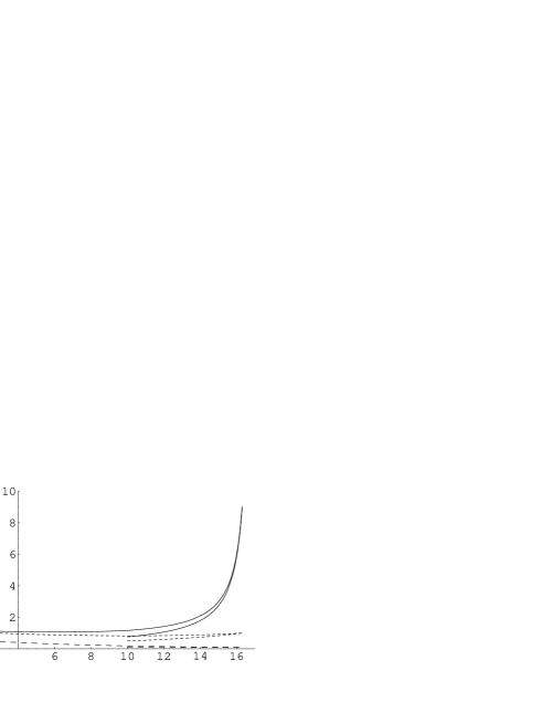
Figure 1: The behavior of the running couplings of $y_{t}$ and $y_{\nu}$ in the ESSM for the initial values, $y_{t}=y_{\nu}=0.3,1$ and 3 at $M_{G}$.

Figure 2: The behavior of the running couplings of $y_{t}$ and $y_{\nu}$ in the MSSM for the initial values, $y_{t}=y_{\nu}=0.3,1$ and 3 at $M_{G}$.

Figure 3: An example of the $M_{R}$ dependence of the predicted value $R(M_{Z})$ in the ESSM (for $\alpha_{3}(M_{Z})=0.12$).

Figure 4: An example of the predicted value of $R(M_{Z})$ in the MSSM (for $\alpha_{3}(M_{Z})=0.12$). The values of $M_{R}$ are as in Fig. 3. The dotted line shows the experimental upper bound on $R(M_{Z})$.

Figure 5: An example of the predicted value of $R(M_{Z})$ in the ESSM for small $\tan\beta$ case (for $\alpha_{3}(M_{Z})=0.12$). The values of $M_{R}$ are as in fig. 3.

References

- [1] C. Giunti, C.W. Kim and U.W. Lee, Mod. Phys. Lett. A6 (1991) 1745; J. Ellis, S. Kelley and D.V. Nanopoulos, Phys. Lett. 260B (1991) 131; U. Amaldi, W. de Boer and H. Fürstenau, Phys. Lett. 260B (1991) 447; P. Langacker and M. Luo, Phys. Rev. D44 (1991) 817
- [2] H. Arason et al., Phys. Rev. Lett. 67 (1991) 2933; V. Barger, M.S. Berger and P. Ohmann, Phys. Rev. D47 (1993) 1093; M. Carena, S. Pokorski and C.E.M. Wagner, Nucl. Phys. B406 (1993) 59; V. Barger, M.S. Berger, P. Ohmann and R.J.N. Phillips, Phys. Lett. 314B (1993) 351
- [3] Particle Data Group, Phys. Rev. D54 (1996) 1; H. Fusaoka and Y. Koide, Phys. Rev. D57 (1998) 3986
- [4] T. Kajita, talk given at Neutrino 98, Takayama, Japan, June 1998; The Super-Kamiokande Collaboration, Phys. Rev. Lett. 81 (1998) 1562
- [5] T. Yanagida, in Proceedings of the Workshop on the Unified Theory and Baryon Number in the Universe, eds. O. Sawada and A. Sugamoto (KEK report 79-18, 1979); M. Gell-Mann, P. Ramond and R. Slansky, in Supergravity, eds. P. van Nieuwenhuizen and D.Z. Freedman (North Holland, Amsterdam, 1979)
- [6] J.A, Holtzman and J.R. Primack, Astrophys. J. 405 (1993) 428; A. Klypin, J. Holtzman, J. Primack and E. Regös, Astrophys. J. 416 (1993) 1; J.R. Primack, J. Holtzman, A. Klypin and D.O. Caldwell, Phys. Rev. Lett. 74 (1995) 2160
- [7] M. Fukugita and T. Yanagida, Phys. Lett. 174B (1986) 45; B.A. Campbell, S. Davidson and K.A. Olive, Nucl. Phys. B399 (1993) 111; H. Murayama and T. Yanagida, Phys. Lett. 322B (1994) 349; W. Buchmuller and M. Plumacher, Phys. Lett. 389B (1996) 73
- [8] H. Murayama, H. Suzuki, T. Yanagida and J. Yokoyama, Phys. Rev. Lett. 70 (1993) 1912
- [9] F. Vissani and A.Yu. Smirnov, Phys. Lett. 341B (1994) 173
- [10] A. Brignole, H. Murayama and R. Rattazzi, Phys. Lett. 335B (1994) 345
- [11] A.Yu. Smirnov, Nucl. Phys. B466 (1996) 25; M. Bando, T. Kugo and K. Yoshioka, Phys. Rev. Lett. 80 (1998) 3004
- [12] A. Giveon, L.J. Hall and U. Sarid, Phys. Lett. 271B (1991) 138
- [13] P. Langacker and N. Polonsky, Phys. Rev. D49 (1994) 1454; N. Polonsky, Phys. Rev. D54 (1996) 4537; B. Brahmachari, hep-ph/9706495
- [14] N.G. Deshpande, B. Dutta and E. Keith, Phys. Lett. 384B (1996) 116; ibid. 388B (1996) 605
- [15] L. Maiani, G. Parisi and R. Petronzio, Nucl. Phys. B136 (1978) 115; D. Ghilencea, M. Lanzagorta, G.G. Ross, Phys. Lett. B415 (1997) 253
- [16] T. Moroi, H. Murayama and T. Yanagida, Phys. Rev. D48 (1993) 2995; B. Brahmachari, U. Sarkar and K. Sridhar, Mod. Phys. Lett. A8 (1993) 3349; K.S. Babu and J.C. Pati, Phys. Lett. 384B (1996) 140
- [17] M. Bando, J. Sato, T. Onogi and T. Takeuchi, Phys. Rev. D56 (1997) 1589
- [18] M. Lanzagorta and G.G. Ross, Phys. Lett. 349B (1995) 319; B.C. Allanach and S.F. King, Nucl. Phys. B473 (1996) 3; ibid. B507 (1997) 91; M. Bando, J. Sato and K. Yoshioka, Prog. Theor. Phys. 98 (1997) 169
- [19] L.J. Hall, R. Rattazzi and U. Sarid, Phys. Rev. D50 (1994) 7048; M. Carena, S. Pokorski, M. Olechowski and C.E.M. Wagner, Nucl. Phys. B426 (1994) 269; D.M. Pierce, J.A. Bagger, K.T. Matchev, R.-J. Zhang, Nucl. Phys. B491 (1997) 3
- [20] C.T. Hill, Phys. Rev. D24 (1981) 691