Gluon plasmon frequency near the light-cone

Abstract

Thermal perturbation theory based on the resummation scheme by Braaten and Pisarski suffers from unscreened collinear singularities whenever outer momenta become light-like. A recently proposed improvement of the hard thermal loops by an additional resummation of an asymptotic mass promises to solve this problem. Here we present a detailed investigation of the next-to-leading order plasmon self-energy. It demonstrates the applicability and consistency of the improved scheme.

I Introduction

The resummation scheme by Braaten and Pisarski [1] is well established in high temperature field theory. Since its first announcement in 1989 it has been applied to a vast variety of physical problems [2], where the calculation of the gluon damping rate was the most spectacular one [3]. To obtain consistent results in a perturbative calculation one has to distinguish two momentum scales. On the hard scale, where momenta are $\sim T$ ($T=$ temperature), the conventional perturbation series is valid. On the soft scale, where the momenta are $\sim gT$ ($g$ is the small coupling), one has to resum the so called ’hard thermal loops’ (HTL). The resulting effective vertices and propagators are screening formerly untreatable infrared singularities. This leads to finite and gauge invariant outcomings for physical quantities.

In some cases, however, it turned out that the HTL were insufficient to screen all infinities. For example, the damping rate of dynamical gluons and the screening length in a gluon plasma suffer from the lack of a thermal magnetic mass [4], which results in an infrared singularity. Another shortcoming was introduced by the HTL itself. Whenever outer momenta are soft and lightlike, the HTL cause collinear singularities [5, 6, 7]. Nevertheless, in a medium like the gluon plasma there are no long range forces since medium effects care for the screening. Thus, such singularities should be spurious.

The Braaten-Pisarski scheme can be understood in the context of a renormalisation group treatment [8]. The effective propagators and vertices are included in an effective action [9] which is the result of integrating out the hard momentum scale. It was shown in [6], however, that in this action for lightlike outer momenta the hard modes have not been integrated out completely. One has to take into account a certain asymptotic thermal mass. An improved HTL resummation scheme has been proposed recently in [10] which includes this mass and is free from collinear singularities while retaining the structure and simplicity of the action [9]. In this letter we will test the new resummation scheme for consistency. Its applicability will be shown by a simple check of the next-to-leading order plasmon frequency.

The paper starts with a collection of notations (sect. 2). The next two sections review a few facts on the plasmon-frequency at next-to-leading order (sect. 3) and on the resummation of asymptotic masses (sect. 4). In section 5 we derive two consistency conditions which the plasmon frequency must obey and in section 6 we test these conditions by explicitly calculating the plasmon frequency near the light-cone. It will be seen that the conditions are fulfilled. Conclusions are given in section 7.

II Notations

Consider a system of gluons in thermal equilibrium at high temperature $T$. It is described by the Lagrangian ${\cal L}=-{1\over 4}F_{\mu\nu}^{a}F^{{\mu\nu}a}-\frac{1}{2\alpha}\left(\partial^{\mu}A_{\mu}^{a}\right)+{\cal L}_{\rm ghost}$ where $F_{\mu\nu}^{a}$ is the non-abelian $SU(N)$ field tensor. The coupling $g$ is small. For simplicity we do not allow for quarks. In the imaginary time formalism each four momentum reads $Q=(Q_{o},\vec{q})$. $Q_{o}=i\omega_{n}=2\pi inT$ are the Matsubara frequencies. We use the metric $g_{\mu\nu}=(+---)$ and a covariant gauge-fixing with parameter $\alpha$.

The spectra of physical exitations in the plasma are defined by the poles of the response function $\chi(\omega,q)=G(Q_{o}\to\omega+i\eta,q)$, ($\eta\to+0$), where $G$ is the gluon propagator. The HTL resummed leading order of $G$ at soft momentum reads

$${}^{*}G_{\mu\nu}(P) = A_{\mu\nu}(P)\Delta_{t}(P)+B_{\mu\nu}(P)\Delta_{l}(P)$$ (2)

$$+\alpha D_{\mu\nu}(P)\Delta_{o}(P)$$

with $\Delta_{t,\ell}:=[P^{2}-\Pi_{t,\ell}]^{-1}$, $\Delta_{o}=1/P^{2}$, $\Pi_{t}:=\frac{1}{2}{\rm Tr}\,(A\Pi)$ and $\Pi_{\ell}:={\rm Tr}\,(B\Pi)$. The Lorentz-matrices are taken from a basis, see eg. [11], where $A$ is the transversal and $B$ is the longitudinal projector.

The propagator has two physical poles [12]. We will concentrate on the longitudinal mode: the solution $\omega_{\ell}(q)$ of

$$\omega_{\ell}^{2}-q^{2} = \Pi_{\ell}(\omega_{\ell},q)\;,$$ (3)

$$\Pi_{\ell}(Q) = -3m^{2}{Q^{2}\over q^{2}}\left\{1-{Q_{o}\over 2q}\ln\left({Q_{o}+q\over Q_{o}-q}\right)\right\}\;,$$ (4)

is the frequency of the well known plasmon [13]. $\Pi_{\ell}$ is the longitudinal part of the polarization function $\Pi_{\mu\nu}$ in HTL approximation. It is the sum of one-loop diagrams where the inner momentum $P$ is hard,

$$\Pi_{\mu\nu}(Q)=2g^{2}N{\textstyle\sum}\!\!\!\!\!\!\int\nolimits_{P}\Delta_{o}^{-}\Delta_{o}\Big{\{}-P^{2}g_{\mu\nu}+2P_{\mu}P_{\nu}\Big{\}}\;.$$ (5)

The summation symbol is defined by ${\scriptstyle\Sigma}\!\!\!\!\int\nolimits_{P}:=\int\!\frac{d^{3}p}{(2\pi)^{3}}T\sum_{n}$ where $n$ runs over all Matsubara frequencies. Throughout the paper $Q$ is the external momentum, $P$ is summed over and $K$ is the difference $K=Q-P$. A superscript ’minus’ refers to the transformation $P\to K$, e.g. $\Delta_{o}^{-}=1/K^{2}$.

As (4) shows, the sumintegral (5) can be performed analytically. But to obtain the Braaten-Pisarski effective action one conveniently starts from

$$\Pi_{\mu\nu}(Q) = 3m^{2}\left(U_{\mu}U_{\nu}-\int_{\Omega}\frac{(UQ)}{(YQ)}Y_{\mu}Y_{\nu}\right)$$ (7)

$$\mbox{with}\quad Y=(1,\vec{e})\quad,\quad m^{2}={g^{2}NT^{2}\over 9}\;.$$

The angular integral $\int_{\Omega}:={1\over 4\pi}\int d^{2}\Omega$ averages over the directions of the unit-vector $\vec{e}$. Using this notation, the effective vertices obtain a pleasant form. They split up into two parts, e.g.

$${}^{*}\Gamma^{(3)}_{{\mu\nu}\sigma}(Q,P,K)=\Gamma^{\rm tree}_{{\mu\nu}\sigma}(Q,P,K)+\delta\Gamma^{(3)}_{{\mu\nu}\sigma}(Q,P,K)\;,$$ (8)

where $\Gamma^{\rm tree}_{{\mu\nu}\sigma}$ is the tree–level and $\delta\Gamma^{(3)}_{{\mu\nu}\sigma}$ the HTL part of the 3-gluon-vertex,

$$\delta\Gamma^{(3)}_{{\mu\nu}\rho} = 3m^{2}\int_{\Omega}{Y_{\mu}Y_{\nu}Y_{\rho}\over YQ}\left\{\frac{P_{o}}{YP}-\frac{K_{o}}{YK}\right\}\;,$$ (9)

$$\delta\Gamma^{(4)}_{{\mu\nu}\rho\lambda} = 6m^{2}\int_{\Omega}{Y_{\mu}Y_{\nu}Y_{\rho}Y_{\lambda}\over(YQ)^{2}}\left\{\frac{P_{o}}{YP}-\frac{K_{o}}{YK}\right\}\;.$$ (10)

For the derivation of the HTL effective action from the above we refer to [9, 10].

III Next to leading order of the Plasmon Frequency

The next to leading order of the plasmon frequency has been extensively studied in [3, 7, 11]. Up to next to leading order the plasmon is the solution of the equation

$$\omega^{2}-q^{2}=\overline{\Pi}_{\ell}(\Omega+i\eta,q)\quad{\rm or}\quad-q^{2}=\overline{\Pi}_{oo}(\Omega+i\eta,q)$$ (11)

since $\Pi_{\mu\nu}$ is transversal up to this order [14, 7]. The complex frequency $\Omega=\omega_{\ell}\,+\,\delta\omega_{\ell}-i\gamma_{\ell}$ is the sum of the plasmon frequency at leading order, its next-to-leading correction and the plasmon damping, while $\overline{\Pi}_{oo}=\Pi_{oo}+\delta\Pi_{oo}$ is the polarization function including next-to-leading order. We expand (11) and find for the physical quantities

$$\delta\omega_{\ell}(q) = -{\Re e\,\delta\Pi_{oo}(\omega_{\ell}+i\eta,q)\over\left.\partial_{\omega}\Pi_{oo}(\omega,q)\right|_{\omega=\omega_{\ell}}}\;,$$ (12)

$$\gamma_{\ell}(q) = {\Im m\,\delta\Pi_{oo}(\omega_{\ell}+i\eta,q)\over\left.\partial_{\omega}\Pi_{oo}(\omega,q)\right|_{\omega=\omega_{\ell}}}\;.$$ (13)

Thus, to calculate $\delta\omega_{\ell}(q)$ or $\gamma_{\ell}(q)$ one has to evaluate $\delta\Pi_{oo}$ and $\Pi_{oo}$ on the leading order mass-shell $\omega=\omega_{\ell}(q)$.

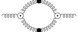
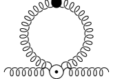
FIG. 1.: The diagrams contributing to the next-to-leading order of the thermal gluon polarization function. The inner momentum is soft, so the propagators and vertices are the resummed ones.

The contributions to $\delta\Pi_{\mu\nu}$ are contained in the diagrams of figure 1,

$$\delta\Pi_{\mu\nu}(Q)=\Pi^{\rm loop}_{\mu\nu}(Q)+\Pi^{\rm tad}_{\mu\nu}(Q)-\Pi^{\rm[-]}_{\mu\nu}(Q)$$ (14)

with

$$\Pi^{\rm loop}_{\mu\nu}(Q) = \frac{1}{2}g^{2}N{\textstyle\sum}\!\!\!\!\!\!\int\nolimits_{P}{}^{*}G^{\rho\sigma}(K){}^{*}G^{\lambda\tau}(P)$$ (16)

$${}^{*}\Gamma_{\mu\rho\lambda}(Q,-K,-P)\,{}^{*}\Gamma_{\nu\sigma\tau}(Q,-K,-P)\;,$$

$$\Pi^{\rm tad}_{\mu\nu}(Q) = \frac{1}{2}g^{2}N{\textstyle\sum}\!\!\!\!\!\!\int\nolimits_{P}{}^{*}G^{\rho\sigma}(P)\,{}^{*}\Gamma_{{\mu\nu}\rho\sigma}(Q,-Q,-P,P)\;.$$ (17)

The two parts $\Pi^{\rm loop}$ and $\Pi^{\rm tad}$ correspond to the two diagrams in figure 1. By subtracting $\Pi^{[-]}$, which is given by figure 1 with hard inner momentum, $\delta\Pi$ is made up of soft inner momenta automatically. The limit of hard momentum, however, does not necessarily imply to replace the resummed propagators and vertices with the tree-level ones. Instead, whenever the outer momentum $Q$ becomes lightlike, one is forced to use massive propagators [10, 15]. We will cover this case in the following section.

IV Resummation of asymptotic masses

For lightlike outer momentum the use of tree-level propagators to obtain $\Pi^{[-]}$ in (14) leads to an incomplete subtraction of the hard momentum scale in the next-to-leading order selfenergy $\delta\Pi$ [6, 10]. Then, strong collinear singularities in $\delta\Pi$ spoil the conventional perturbative expansion.

As an example for the underlying mechanism consider the toy-term

$$\delta\Pi^{\rm Example}=-4e^{2}\!\int\!\!{d^{3}p\over(2\pi)^{3}}{n_{b}(p)\over p}\,\left\{{\vec{p}\vec{q}\over\omega_{p}\omega-\vec{p}\vec{q}}-{\vec{p}\vec{q}\over p\omega-\vec{p}\vec{q}}\right\}$$ (18)

with $\omega_{p}^{2}=p^{2}+m^{2}$. The first part of $\delta\Pi^{\rm Example}$ is typical for the one-loop diagrams in figure 1. For simplicity we have replaced the complicated self-energies by a single mass $m$. The second part is the analogon to $\Pi^{[-]}$ in the tree-level approximation.

When $Q$ is off the light-cone, i.e. $\omega>q$, the leading order of the integral in (18) obviously comes from soft $p$. We can approximately set $n_{b}(p)\approx T/p$ and evaluate (18). But with $Q$ becoming light-like, $\omega\mathrel{\hbox to0.0pt{\raise 2.20013pt\hbox{$>$}\hss}{\lower 2.20013pt\hbox{$\sim$}}}q$, the two parts in (18) behave totally different. The second term becomes large due to a collinear singularity while the first one remains finite. Now, the integration is not any more restricted to the soft scale. Still using $n_{b}(p)\approx T/p$, we find a strong power-like singularity [6],

$$\delta\Pi^{\rm Example} \to -{e^{2}\mu T\over 2\pi}{\omega\over q}\int_{-1}^{1}\!du\,{u^{2}\over{\sqrt{\omega^{2}/q^{2}-u^{2}}}^{3}}\;\sim\;{1\over\varepsilon}$$ (20)

$${\rm with}\quad\varepsilon^{2}={\omega^{2}-q^{2}\over q^{2}}\;.$$

Thus, this behavior is not solely due to a collinear singularity, but also to a latent UV-singularity, which is caused by a premature restriction to soft momenta. Obviously, if $\varepsilon$ becomes sufficiently small, $\delta\Pi$ may overgrow the leading order self-energy $\Pi$ and the perturbative expansions breaks down.

For the consistency of the Braaten-Pisarski effective action [9] the above behavior is a disaster. The hard scale has not been integrated out entirely and consequently the action of [1] is incomplete in the sense of renormalization group theory. To restore consistency, as seen in [10], one has to include a certain asymptotic mass

$$m_{\infty}^{2}=\Pi_{t}(Q^{2}=0)={g^{2}NT^{2}\over 6}$$ (21)

in the calculation of the hard thermal loops. Fortunately, though including $m_{\infty}$, in the corresponding improved HTL-effective action [10] the elegant structure and gauge-invariance of the Braaten-Pisarski action [9] can be maintained. Moreover, recalculating the gluon polarization function with the improved action gives finite results for all momenta, including the light-cone.

V Consistency conditions

The true gluon system has a richer structure than in the previous example. Here, the above mentioned latent UV-singularities are not the only mechanism that cause $\delta\Pi$ to grow near the light-cone. As will be seen in the following section, the HTL-parts of the vertices introduce additional collinear singularities which may cause a breakdown of the perturbation expansion. However, the physical quantity under consideration is not the self-energy, but plasmon frequency and damping. It is shown in this section, that the physical quantities can tolerate a certain amount of light-cone enhancements in the self-energy without spoiling their perturbative expansion.

Consider equation (12) that defines $\delta\omega_{\ell}$ and $\gamma_{\ell}$. For its derivation we made use of two (really trivial) inequalities,

$$\delta\omega_{\ell},\gamma_{\ell}\ll\omega_{\ell}\qquad{\rm and}\qquad\delta\Pi_{oo}\ll\Pi_{oo}$$ (22)

for all physical momenta. Violation of the inequalities (22) would invalidate the perturbative expansion of the physical quantities. In the following section we check (22) by calculating $\delta\Pi_{oo}$ near the light-cone.

However, we will not do the calculation on the light-cone but we will keep a small distance $g\ll\varepsilon\ll 1$ with $\varepsilon^{2}=(\omega^{2}-q^{2})/q^{2}$ for two reasons:

• On the light-cone the use of the improved HTL-vertices [10] is required, leading into technical difficulties. For $\varepsilon\gg g$, however, we may neglect $m_{\infty}$, which renders the following calculation feasible.

• A finite but small distance $\varepsilon\gg g$ is still interesting to decide whether the asymptotic mass resummation is sufficient near the light-cone. If there were a breakdown of perturbation theory (there is none!) we would have to think about an additional resummation to $m_{\infty}$, for example one including some kind of thermal damping, see eg [16]. Such a new screening mechanism for the collinear singularities may show up in a larger (though still small) distance $\varepsilon$, namely $\varepsilon^{2}\sim g$ (rather than $\varepsilon^{2}\sim g^{2}$ in the case of $m_{\infty}$). But this range is consistently treated within the present framework.

Let us return to the conditions (22). Since in (12) we have $\partial_{\omega}\Pi_{oo}\sim g^{2}T^{2}/\varepsilon^{2}$ near the light-cone, the first condition in (22) is a rather weak one for the self-energy $\delta\Pi$. It may behave like

$$\Re e\;\delta\Pi_{oo},\;\Im m\,\delta\Pi_{oo}\sim g^{3}T^{2}{1\over\varepsilon^{2}}$$ (23)

without violating $\delta\omega_{\ell},\gamma_{\ell}\ll\omega_{\ell}$. Even additional logarithms $\ln(\varepsilon)$ are allowed. The second inequality in (22) is more restrictive. The leading order $\Pi_{oo}$ behaves like $\Pi_{oo}\sim g^{2}T^{2}\ln(\varepsilon)$ and thus

$$\Re e\,\delta\Pi_{oo}\mathrel{\hbox to0.0pt{\raise 2.20013pt\hbox{$<$}\hss}{\lower 2.20013pt\hbox{$\sim$}}}g^{3}T^{2}{1\over\varepsilon}$$ (24)

is allowed as long as $\varepsilon\mathrel{\hbox to0.0pt{\raise 2.20013pt\hbox{$>$}\hss}{\lower 2.20013pt\hbox{$\sim$}}}g$. The condition (24) does not apply to the imaginary part because the leading order $\Im m\,\Pi$ is zero for physical momenta.

Combining (23) and (24), we arrive at the following inequalities which form the consistency conditions to be fulfilled by $\delta\Pi_{oo}$ for $g\ll\varepsilon\ll 1$:

$$\Re e\,\delta\Pi_{oo}\mathrel{\hbox to0.0pt{\raise 2.20013pt\hbox{$<$}\hss}{\lower 2.20013pt\hbox{$\sim$}}}g^{3}T^{2}{1\over\varepsilon}\quad{\rm and}\quad\Im m\,\delta\Pi_{oo}\mathrel{\hbox to0.0pt{\raise 2.20013pt\hbox{$<$}\hss}{\lower 2.20013pt\hbox{$\sim$}}}g^{3}T^{2}{1\over\varepsilon^{2}}\;.$$ (25)

These restrictions on the light-cone behavior of $\delta\Pi_{oo}$ will be checked by explicit calculation in the following section.

VI Plasmon frequency near the light-cone

In this main section we evaluate the next-to-leading gluon polarization function $\delta\Pi_{oo}(Q)$ near the light-cone $Q^{2}=0$. We are interested in the order of magnitude of the first term of the asymptotics in $\varepsilon^{2}=Q^{2}/q^{2}$.

The starting point of the calculation is equation (4.5) of [7]. The expression for $\delta\Pi_{oo}$ can be split into two parts,

$$\delta\Pi_{oo}(Q)=:\delta\Pi^{\rm tree}_{oo}(Q)+\delta\Pi^{\rm HTLV}_{oo}(Q)\;.$$ (26)

The first part contains only tree level vertices while all the remaining contributions from HTL-vertices are assembled in $\delta\Pi^{\rm HTLV}_{oo}$. In both parts the propagators are the resummed one (2).

The tree-level part $\delta\Pi^{\rm tree}_{oo}$ has been studied in [7]. There, one obtains the mechanism discussed in section IV leading to the asymptotic mass resummation. With use of the improved HTL effective action [10] this part will be completely finite near the light-cone without including any enhancement effects.

In $\delta\Pi^{\rm HTLV}_{oo}$, however, the HTL-vertices indeed introduce strong collinear effects. This part is given by

$$\delta\Pi_{oo}^{\rm HTLV}(Q)=\Big{\{}\Sigma+\Upsilon+\Phi+\Psi\Big{\}}$$ (27)

with

$$\Sigma = \frac{1}{2}g^{2}N{\textstyle\sum}\!\!\!\!\!\!\int\nolimits_{P}\Delta\delta\Gamma_{oooo}\;,$$ (28)

$$\Upsilon = \frac{1}{2}g^{2}N{\textstyle\sum}\!\!\!\!\!\!\int\nolimits_{P}\Delta\Delta^{-}(\delta\Gamma_{ooo})^{2}\;,$$ (29)

$$\Phi = g^{2}N{\textstyle\sum}\!\!\!\!\!\!\int\nolimits_{P}\Delta_{t}\Delta^{-}\Big{\{}\delta\Gamma_{oo\mu}\delta\Gamma_{oo}{}^{\mu}$$ (31)

$$\quad\qquad+2(P_{o}+Q_{o})\delta\Gamma_{ooo}\Big{\}}\;,$$

$$\Psi = \frac{1}{2}g^{2}N{\textstyle\sum}\!\!\!\!\!\!\int\nolimits_{P}\Delta_{t}\Delta_{t}^{-}\delta\Gamma_{o{\mu\nu}}\delta\Gamma_{o}{}^{\mu\nu}\;,$$ (32)

as well as $\Delta=(\Delta_{t}-\Delta_{\ell})P^{2}/p^{2}$. The HTL-parts of the vertices $\delta\Gamma$ are given by (9) and (10). Remember, $Q$ refers to the outer momentum, $P$ is summed over and $K=Q-P$. We will concentrate on the terms $\Sigma$ and $\Upsilon$ which are the only ones giving rise to strong collinear singularities [17].

For summing over the Matsubara frequencies it is convenient to introduce spectral densities $\Delta(P_{o},p)=\int\!dx\,\rho(x,p)/(P_{o}-x)$. The explicit form of $\rho$ is given e.g. in appendix B of [11]. Since in $\delta\Pi^{\rm HTLV}_{oo}$ the variables $p$ and $x$ are soft from the outset we may use $n_{b}(x)\approx{T\over x}$.

$$\Sigma = g^{2}NT\int\!\!{d^{3}p\over(2\pi)^{3}}\,\int\!\!dx\,{\varrho(x,p)\over x}$$ (34)

$$\int_{\Omega}{3m^{2}\over(YQ)^{2}}{Q_{o}\over Q_{o}-x-\vec{e}\vec{k}}\;,$$

$$\Upsilon = -g^{2}NT\int\!\!{d^{3}p\over(2\pi)^{3}}\,\int\!\!dxdy{\varrho(x,p)\varrho(y,k)\over Q_{o}-x-y}$$ (37)

$$\int_{\Omega\Omega^{\prime}}{3m^{2}\over YQ}{3m^{2}\over Y^{\prime}Q}\left\{{1\over x}{Q_{o}-x\over Q_{o}-x-\vec{e}\vec{k}}{Q_{o}\over Q_{o}-x-\vec{e}^{\prime}\vec{k}}\right.$$

$$\left.-2{Q_{0}\over Q_{o}-\vec{e}\vec{p}-\vec{e}^{\prime}\vec{k}}{1\over Q_{o}-x-\vec{e}^{\prime}\vec{k}}\right\}\;.$$

At this stage we are allowed to perform the analytical continuation $Q_{o}\to\omega+i\eta$, $\eta\to+0$. In the following we keep with the notation $Q_{o}$ but always mean $\omega+i\eta$.

As we will see in the next subsection the main reason for the strong light-cone singularities is a combination of collinear and infrared effects. This is due to the weird behavior of the transversal density [11] for small momentum,

$${\varrho_{t}(x,p)\over x}\to{1\over p^{2}}\delta(x)\qquad{\rm for}\qquad p\to 0\;,$$ (38)

which is nothing but the lack of a magnetic screening mass. We split off the IR-sensitive part,

$$\Sigma=\Sigma_{o}+(\Sigma-\Sigma_{o})=\Sigma_{o}+\Sigma_{1}\>,$$ (39)

$$\Upsilon=2\Upsilon_{o}+(\Upsilon-2\Upsilon_{o})=2\Upsilon_{o}+\Upsilon_{1}$$ (40)

where the factor 2 in the second equation is for conveniance. It comes from the fact that $\Upsilon$ is invariant with respect to the interchange $\vec{p}\to\vec{k}$. So, we have two infrared regions, $p\to 0$ as well as $k\to 0$. Using (38) to neglect $x$, the IR-sensitive parts are given by

$$\Sigma_{o} = g^{2}NT\int\!\!{d^{3}p\over(2\pi)^{3}}\,\int\!\!dx\,{\varrho(x,p)\over x}$$ (42)

$$\int_{\Omega}{3m^{2}\over(YQ)^{2}}{Q_{o}\over Q_{o}-\vec{e}\vec{k}}\;,$$

$$\Upsilon_{o} = -g^{2}NT\int\!\!{d^{3}p\over(2\pi)^{3}}\,\int\!\!dxdy\,{\varrho(x,p)\varrho(y,k)\over x\;(Q_{o}-y)}$$ (44)

$$\int_{\Omega\Omega^{\prime}}{3m^{2}\over YQ}{3m^{2}\over Y^{\prime}Q}{Q_{o}\over Q_{o}-\vec{e}\vec{k}}{Q_{o}\over Q_{o}-\vec{e}^{\prime}\vec{k}}\;.$$

In fact, these parts are the only ones showing a strong light-cone behavior [17]. We will concentrate on them. The remaining terms $\Sigma-\Sigma_{o}$ and $\Upsilon-2\Upsilon_{o}$ are of no relevance in the present context.

A Evaluation of $\Sigma_{o}$

We start with the simpler one of the two contributing parts. In (42) the $x$-integration is performed using sum-rules derived eg. in [18, 11].

$$\Sigma_{o}=g^{2}NT\int\!\!{d^{3}p\over(2\pi)^{3}}{1\over p^{2}}{3m^{2}\over p^{2}+3m^{2}}\int_{\Omega}{3m^{2}\over(YQ)^{2}}{Q_{o}\over YQ+\vec{e}\vec{p}}$$ (45)

with rewriting $Q_{o}-\vec{e}\vec{k}=YQ+\vec{e}\vec{p}$. Near the light-cone $Q^{2}=0$ the denominator $(YQ)^{2}$ tends to diverge. At $YQ=Q_{o}-\vec{e}\vec{q}=0$ it gives rise for a powerlike collinear singularity. In addition, the second denominator in (45), $YQ+\vec{e}\vec{p}$, mixes the collinear point $YQ=0$ with the infrared region of the $p$ integration. For vanishing $YQ$ we obtain a logarithmic singularity at small $p$, for vanishing $p$ the collinear singularity becomes stronger. So, from (45) we expect the leading contribution to come from a very limited region of the integration variables: the infrared limit of the $p$-Integral.

More precisely, after performing the angular integration, we have

$$\Sigma_{o}=g^{2}NT\int\!\!{d^{3}p\over(2\pi)^{3}}{1\over p^{2}}{3m^{2}\over p^{2}+3m^{2}}{m_{\infty}^{2}\omega^{2}(\vec{p}\vec{q}-p^{2})\over{\sqrt{(\vec{p}\vec{q})^{2}+Q^{2}p^{2}}}^{3}}$$ (47)

$$\left\{\ln\left({Q^{2}+\vec{p}\vec{q}+\sqrt{\phantom{x}}\over Q^{2}+\vec{p}\vec{q}-\sqrt{\phantom{x}}}\right)-i\pi\Theta\left(p^{2}-2\vec{p}\vec{q}-Q^{2}\right)\right\}\;.$$

Indeed, $Q^{2}$ regulates the infrared behavior of the $p$-integral, as we can see in particular in the step-function of the imaginary part of (47). The leading contribution of the light-cone asymptotics comes from $p^{2}$ and $\vec{p}\vec{q}$ becoming comparable small to $Q^{2}$.

Accordingly we scale $p\to\varepsilon qv$ and $\vec{p}\vec{q}/pq\to\varepsilon u$. Now the integration variables are dimensionless.

$$\Sigma_{o} = {1\over\varepsilon^{2}}\Gamma\int_{0}^{\infty}\!\!dv\int_{-1/\varepsilon}^{1/\varepsilon}\!\!du{\alpha^{2}\over v^{2}+\alpha^{2}}{u-v\over v^{2}{\sqrt{1+u^{2}}}^{3}}$$ (49)

$$\left\{\ln\left({{1\over v}+u+\sqrt{\phantom{x}}\over{1\over v}+u-\sqrt{\phantom{x}}}\right)-i\pi\Theta\left(v^{2}-2uv-1\right)\right\}$$

with $\Gamma={g^{2}NTm_{\infty}^{2}/(4\pi^{2}q)}$ and $\alpha^{2}={3m^{2}/(\varepsilon^{2}q^{2})}$. The latter constant $\alpha$, becomes large near the light-cone. However, we are not allowed to perform $\alpha\to\infty$ since a finite $\alpha$ is needed to control the $v$-integral for large values of $v$. Nevertheless, evaluating (49) analytically,

$$\Im m\,\Sigma_{o} = \pi\Gamma\left(\ln(\alpha^{2}/\rho)-2+{\cal O}(\varepsilon^{2})\right)$$ (50)

$$= \pi\Gamma\left(\ln({12m^{2}\over q^{2}\varepsilon^{4}})-2+{\cal O}(\varepsilon^{2})\right)\;,$$ (51)

$$\Re e\,\Sigma_{o} = {1\over\varepsilon^{2}}\Gamma\left(-\pi^{2}+{\cal O}(\varepsilon^{2})\right)\;,$$ (52)

with $\rho=(\sqrt{1+\varepsilon^{2}}-1)/(\sqrt{1+\varepsilon^{2}}+1)\sim\varepsilon^{2}/4$. Indeed, we obtain strong collinear singularities $\sim\varepsilon^{-2}$. For the real part, the result (52) violates, if considered separately, the inequality (25) given in the last section. Thus, assuming (52) is the final result, the perturbative expansion of the physical quantities $\omega_{\ell}$ and $\gamma_{\ell}$ would be broken.

B Evaluation of $\Upsilon_{o}$

Compared to $\Sigma_{o}$ the evaluation of $\Upsilon_{o}$ is more involved due to the additional propagator $\Delta^{-}$ in (29). Before we discuss simplifications for $\Delta^{-}$ we turn to (44), apply the sum rules and perform the angular integrations.

$$\Upsilon_{o}=\frac{1}{2}g^{2}NT\int\!\!{d^{3}p\over(2\pi)^{3}}{1\over p^{2}}{3m^{2}\over p^{2}+3m^{2}}{\Delta(Q_{o},k)m_{\infty}^{4}\omega^{2}\over\sqrt{(\vec{p}\vec{q})^{2}+\varepsilon^{2}p^{2}q^{2}}{}^{2}}$$ (54)

$$\left\{\ln\left({Q^{2}+\vec{p}\vec{q}+\sqrt{\phantom{x}}\over Q^{2}+\vec{p}\vec{q}-\sqrt{\phantom{x}}}\right)-i\pi\Theta\left(p^{2}-2\vec{p}\vec{q}-Q^{2}\right)\right\}^{\displaystyle 2}\;.$$

Despite of the additional propagator, (54) has the same structure than $\Sigma_{o}$ in (45). Indeed, the leading $\varepsilon$-order of $\Upsilon_{o}$ comes from the same very limited region of the integration variables as in $\Sigma_{o}$: $p^{2}$ as well as $\vec{p}\vec{q}$ are comparable small to $Q^{2}$. This opens the possibility for suitable approximations in the propagator $\Delta^{-}$.

1 The propagator

The propagator $\Delta$ in (54) is made up of two parts,

$$\Delta(Q_{o},k) = {1\over k^{2}}\left\{{Q_{o}^{2}-k^{2}\over Q_{o}^{2}-k^{2}-\Pi_{t}}\right.$$ (56)

$$\left.-{Q_{o}^{2}-k^{2}\over(Q_{o}^{2}-k^{2})(1+\Pi_{oo}/k^{2})}\right\}\;.$$

The transversal part (first term) does not contribute to the leading order since its numerator behaves like $Q^{2}$ and in the denominator $\Pi_{t}$ does not vanish for $Q_{o}\approx k$. Hence,

$$\Delta(Q_{o},k)\approx{-1\over k^{2}+3m^{2}\left[1-\frac{1}{2}{Q_{o}\over k}\ln\left({Q_{o}+k\over Q_{o}-k}\right)\right]}\;.$$ (57)

When we do the analytical continuation $Q_{o}\to\omega+i\eta$ ($\eta\to+0$) the denominator has besides the common [4] $i\sigma\eta$, $\sigma=\pm 1$ a further imaginary part from the cut of the logarithm,

$$\ln\left({Q_{o}+k\over Q_{o}-k}\right)\to\ln\left|{\omega+k\over\omega-k}\right|-i\pi\Theta(k^{2}-\omega^{2})\;.$$ (58)

Thus

$$\Delta(\omega,k)\approx{-1\over k^{2}+\Pi_{oo}(\omega,k)+i\pi m_{\infty}^{2}{\omega\over k}\Theta(k^{2}-\omega^{2})+i\eta\sigma}\;.$$

With regard to the value of the step function $\Theta$ we distinguish two cases.

$\Theta=0$ ($k^{2}<\omega^{2}$). In this case

$$\Delta_{0} = {-1\over k^{2}+\Pi_{oo}(\omega,k)}+i\pi\sigma\delta\left(k^{2}+\Pi_{oo}\right)$$ (59)

$$= {-1\over k^{2}+\Pi_{oo}(\omega,k)}+i\pi\sigma{\delta(k^{2}-q^{2})\over|1+\partial_{q^{2}}\Pi_{oo}(\omega,q)|}\;.$$ (60)

Near the light-cone we have $\sigma=1$ and $\partial_{q^{2}}\Pi_{oo}=-m_{\infty}^{2}/Q^{2}$. Remember, we have to evaluate $\delta\Pi$ on the longitudinal mass-shell, see (12). Thus $\omega=\omega_{\ell}(q)$ is given and $k^{2}+\Pi_{oo}(\omega,k)$ is zero at $k^{2}=q^{2}$, because this is the longitudinal mass-shell condition defining $\omega_{\ell}$.

In the term of (60) with the delta-function we will find the known problems with the mass shell singularity. Here the only true IR-divergence will occur following the mechanism described in [4]. We will regulate this by including an artificial small cut-off mass $\mu$. All the other parts of $\Upsilon$ are IR-finite and do not need any $\mu$.

$\Theta=1$ ($k^{2}>\omega^{2}$). In this case we are allowed to neglect $i\eta$ in the denominator,

$$\Delta_{1}={-1\over k^{2}+\Pi_{oo}(\omega,k)+i\pi m_{\infty}^{2}{\omega\over k}}\;.$$ (61)

In both cases we simplify $k^{2}+\Pi_{oo}$ using $q^{2},m^{2}\gg p^{2}-2\vec{p}\vec{q}$. As mentioned above we must avoid the use of $Q^{2}\gg p^{2}-2\vec{p}\vec{q}$. In addition we take advantage of being on the longitudinal mass-shell $q^{2}+3m^{2}\left[1-\frac{1}{2}{\omega\over q}\ln\left({\omega+q\over\omega-q}\right)\right]=0$. We obtain

$$k^{2}+\Pi_{oo}(\omega,k)$$ (62)

$$= (\vec{q}-\vec{p})^{2}+3m^{2}\left[1-{\omega/2\over\sqrt{(\vec{q}-\vec{p})^{2}}}\ln\left({\omega+\sqrt{\phantom{x}}\over\omega-\sqrt{\phantom{x}}}\right)\right]$$ (63)

$$\approx {3\over 2}m^{2}\ln\left({\omega^{2}-k^{2}\over Q^{2}}\right)\;.$$ (64)

This simplification, to be used in (60) and (61), makes the following integrals feasible.

2 $\Theta=0$ part of $\Upsilon_{o}$

We turn to the evaluation of $\Upsilon_{o}$. For convenience the distinction of the two cases $\Theta=0$ and $\Theta=1$ will be retained. Accordingly we split $\Upsilon_{o}$ into two parts

$$\Upsilon_{o}=\Upsilon_{o}^{\Theta=0}+\Upsilon_{o}^{\Theta=1}\;.$$ (65)

Both parts are now evaluated separately.

The part with vanishing step-function is given by

$$\Upsilon_{o}^{\Theta=0} = \frac{1}{2}g^{2}NT\int\!\!{d^{3}p\over(2\pi)^{3}}{1\over p^{2}}{3m^{2}\over p^{2}+3m^{2}}{m_{\infty}^{4}\omega^{2}\over\sqrt{(\vec{p}\vec{q})^{2}+\varepsilon^{2}p^{2}q^{2}}^{\displaystyle 2}}$$ (68)

$$\ln^{2}\left({Q^{2}+\vec{p}\vec{q}+\sqrt{\phantom{x}}\over Q^{2}+\vec{p}\vec{q}-\sqrt{\phantom{x}}}\right)\Theta(\omega^{2}-k^{2})$$

$$\left\{{-1\over m_{\infty}^{2}\ln\left({\omega^{2}-k^{2}\over Q^{2}}\right)}+{i\pi\sigma\delta(k^{2}-q^{2})\over[1+\partial_{q}^{2}\Pi_{oo}(\omega,q)]}\right\}\;.$$

First consider the real part of (68). Scaling $p\to\varepsilon qv$ and $\vec{p}\vec{q}/pq\to\varepsilon u$ we have

$$\Re e\;\Upsilon_{o}^{\Theta=0}={\Gamma\over 2\varepsilon^{2}}\int_{o}^{\infty}\!\!dv{1\over v^{2}}{\alpha^{2}\over v^{2}+\alpha^{2}}\int_{-1/\varepsilon}^{1/\varepsilon}\!\!du{1\over u^{2}+1}$$ (70)

$${\Theta(1+2uv-v^{2})\over\ln(1+2uv-v^{2})}\ln^{2}\left({1/v+u+\sqrt{u^{2}+1}\over 1/v+u-\sqrt{u^{2}+1}}\right)$$

where $\Gamma={g^{2}NTm_{\infty}^{2}/(4\pi^{2}q)}$ and $\alpha^{2}={3m^{2}/(\varepsilon^{2}q^{2})}$ are the notations we used in (49). Contrary to (49), the $v$-integral now is finite at both limits small and large $v$. For large $v$ it is cut by the step-function. So, here we are allowed to perform $\alpha^{2}\to\infty$. The fact that (70) is well behaved at $v=0$ is seen by expanding the logarithms in $v^{2}$ and $uv$.

By substituting $v\to\sqrt{1+u^{2}}v-u$ and $t=u/\sqrt{\phantom{x}}$, symmetrizing in $t$ and $v$ as well as introducing $x=(1-v)/(1+v)$ and $y=(1-t)/(1+t)$, we obtain

$$\Re e\,\Upsilon_{o}^{\Theta=0} = -{1\over 2\varepsilon^{2}}\Gamma\int_{0}^{1}\!\!dx\int_{\rho}^{1}\!\!dy{1\over(x-y)^{2}(1-xy)^{2}}$$ (72)

$${(x-y)^{2}\ln^{2}(xy)+(1-xy)^{2}\ln^{2}(x/y)\over\ln(x/y)-2\ln\left({1+x\over 1+y}\right)}$$

with $\rho=(\sqrt{1+\varepsilon^{2}}-1)/(\sqrt{1+\varepsilon^{2}}+1)\approx\varepsilon^{2}/4$. However, the integrand $F(x,y)$ is singular at the origin $(x,y)=0$ and we are not allowed to neglect $\rho$ here. Instead, we exploit $F(x,y)$ being antisymmetric with respect to interchange of $x$ and $y$, $F(x,y)=-F(y,x)$. Hence,

$$\Re e\,\Upsilon_{o}^{\Theta=0}={1\over 2\varepsilon^{2}}\Gamma\int_{\rho}^{1}\!\!dx\int_{o}^{\rho}\!\!dy\,F(x,y)\;.$$ (73)

After scaling both integration-variables $x$ and $y$ with $\rho$ it is finally possible to neglect $\rho\sim\varepsilon^{2}$ in the remaining integral. After another change of variables $x\to 1/x$ we obtain the result for the real part of $\Upsilon_{o}^{\Theta=0}$,

$$\Re e\,\Upsilon_{o}^{\Theta=0} = -{1\over 2\varepsilon^{2}}\Gamma\int_{o}^{1}\!\!dx\int_{o}^{1}\!\!dy{\ln(xy)\over(1-xy)^{2}}$$ (74)

$$= {1\over\varepsilon^{2}}\Gamma\;{\pi^{2}\over 6}\;.$$ (75)

Obviously, we have found one more term $\sim\varepsilon^{-2}$ in the real part of $\delta\Pi_{oo}$ which, if considered separately, would spoil the common perturbation theory.

We turn to the imaginary part of $\Upsilon_{o}^{0}$. Here we find the only true infrared problem due to a mass-shell singularity [4]. It needs an artificial infrared regulator in the transversal part of the propagator, $\Delta_{t}(P_{o}=0)=-(\vec{p}^{2}+\mu^{2})^{-1}$. Consider the mass $\mu$ to be small compared to the soft scale ($\mu\ll gT$) as well as $\mu/\varepsilon\ll gT$. With the latter condition we again restrict ourself to a distance $\varepsilon$ with $g\ll\varepsilon\ll 1$. While in section 5 we used this restrictions to neglect the asymptotic mass in the HTL- propagators and -vertices (otherwise the present calculation would have been undoable) we now need it to solve the integral in (77).

In $\Im m\,\Upsilon_{o}^{\Theta=0}$ we first exploit the delta-function in (68). Then we proceed as with the real part. Scaling $p\to\varepsilon qv$ and with $\alpha^{2}\to\infty$ we obtain

$$\Im m\,\Upsilon_{o}^{\Theta=0} = {g^{2}NT\over(2\pi)^{2}}{m_{\infty}^{2}\omega^{2}\over\varepsilon^{2}q^{3}}{\pi\sigma m_{\infty}^{2}\over\varepsilon^{2}q^{2}|1+\partial_{q}^{2}\Pi_{oo}|}{1\over 4}\int_{0}^{1/\varepsilon}\!\!dv$$ (77)

$${1\over v}{1\over v^{2}+1}{1\over v^{2}+b^{2}}\ln^{2}\left({\sqrt{v^{2}+1}+v\over\sqrt{v^{2}+1}-v}\right)$$

where the dependence on the artificial infrared cutoff $\mu$ is contained in $b^{2}=\mu^{2}/(4q^{2}\varepsilon^{2})$. While $b$ is small, see above, the $b$-asymptotics of the $v$-integral can be calculated analytically. We finally obtain for the imaginary part of $\Upsilon_{o}^{\Theta=0}$

$$\Im m\,\Upsilon_{o}^{\Theta=0}=-\pi{\Gamma\over 2\varepsilon^{2}}\left\{\ln\left(\mu^{2}\over q^{2}\varepsilon^{2}\right)+{7\over 4}\zeta(3)-3\right\}\;.$$ (78)

The logarithm, containing the $\mu$-dependence, is known from several work on plasmon-damping [4].

3 $\Theta=1$ part of $\Upsilon_{o}$

With the propagator $\Delta_{1}$ from (61) our starting point reads

$$\Upsilon_{o}^{\Theta=1}=\frac{1}{2}g^{2}NT\int\!\!{d^{3}p\over(2\pi)^{3}}{1\over p^{2}}{3m^{2}\over p^{2}+3m^{2}}{m_{\infty}^{2}\omega^{2}\over\sqrt{(\vec{p}\vec{q})^{2}+\varepsilon^{2}p^{2}q^{2}}{}^{\displaystyle 2}}$$ (80)

$${-\Theta(k^{2}-\omega^{2})\over\ln\left({\omega^{2}-k^{2}\over Q^{2}}\right)+i\pi\omega/k}\left\{\ln\left({Q^{2}+\vec{p}\vec{q}+\sqrt{\phantom{x}}\over Q^{2}+\vec{p}\vec{q}-\sqrt{\phantom{x}}}\right)-i\pi\right\}^{\displaystyle 2}\!\!.$$

Following the transformations and substitutions known from evaluating $\Re e\,\Upsilon_{o}^{\Theta=0}$, we obtain

$$\Upsilon_{o}^{\Theta=1} = -{\Gamma\over 2\varepsilon^{2}}\int_{0}^{1}\!\!dx\int_{\rho}^{1}\!\!dy{1\over{\cal L}+i\pi}$$ (82)

$$\left\{{(\ln(xy)+i\pi)^{2}\over(1+xy)^{2}}+{\left(\ln\left({x\over y}\right)+i\pi\right)^{2}\over(x+y)^{2}}\right\}$$

where ${\cal L}=\ln\left({x(1+y)^{2}\over y(1-x)^{2}}\right)$. Splitting in real and imaginary part,

$$\Upsilon_{o}^{\Theta=1}=-{\Gamma\over 2\varepsilon^{2}}\int_{0}^{1}\!\!dx\int_{\rho}^{1}\!\!dy\,{F_{R}(x,y)-i\pi F_{I}(x,y)\over{\cal L}^{2}+\pi^{2}}\;,$$ (83)

$$F_{R}(x,y) = {\left(\ln^{2}(xy)-\pi^{2}\right){\cal L}+2\pi^{2}\ln(xy)\over(1+xy)^{2}}$$ (85)

$$+{\left(\ln^{2}\left({x\over y}\right)-\pi^{2}\right){\cal L}+2\pi^{2}\ln\left({x\over y}\right)\over(x+y)^{2}}\;,$$

$$F_{I}(x,y) = {\ln^{2}(xy)-2{\cal L}\ln(xy)-\pi^{2}\over(1+xy)^{2}}$$ (87)

$$+{\ln^{2}\left({x\over y}\right)-2{\cal L}\ln\left({x\over y}\right)-\pi^{2}\over(x+y)^{2}}\;.$$

As both functions $F(x,y)$ are singular at the origin $(x,y)=0$, we are not allowed to neglect $\rho\sim\varepsilon^{2}$. Instead, we isolate the singular parts (index $),

$$F_{R}^{\$}(x,y) = {\ln\left({x\over y}\right)({\cal L}^{2}+\pi^{2})\over(x+y)^{2}}\;,$$ (88)

$$F_{I}^{\$}(x,y) = -{{\cal L}^{2}+\pi^{2}\over(x+y)^{2}}\;.$$ (89)

These parts can easily be integrated over,

$$\int_{0}^{1}\!\!dx\int_{\rho}^{1}\!\!dy\,{\ln\left({x\over y}\right)\over(x+y)^{2}} = -{\pi^{2}\over 6}+{\cal O}(\rho\ln(\rho))\;,$$ (90)

$$\int_{0}^{1}\!\!dx\int_{\rho}^{1}\!\!dy\,{-1\over(x+y)^{2}} = \ln(\rho)+\ln(2)+{\cal O}(\rho)\;.$$ (91)

In the remaining integrals the differences $F-F^{\$}$ are regular on the entire $(x,y)$-interval. So, for the leading term of the $\varepsilon$-asymptotic we are now allowed to set $\rho=0$. Nevertheless, the integrals are not trivial at all. For technical details we refer to the appendix. The result of the calculation is,

$$\int_{0}^{1}\!\!dx\,dy\,{F_{R}(x,y)-F_{R}^{\$}(x,y)\over{\cal L}^{2}+\pi^{2}} = -{\pi^{2}\over 2}\;,$$ (92)

$$\int_{0}^{1}\!\!dx\,dy\,{F_{I}(x,y)-F_{I}^{\$}(x,y)\over{\cal L}^{2}+\pi^{2}} = {7\over 4}\zeta(3)-\ln(2)-1\;.$$ (93)

Combining these parts to $\Upsilon_{o}^{\Theta=1}$ we find for the real and imaginary part

$$\Re e\,\Upsilon_{o}^{\Theta=1}=-{\Gamma\over 2\varepsilon^{2}}\left\{\;,-{2\pi^{2}\over 3}\;,\right\}\;,$$ (94)

$$\Im m\,\Upsilon_{o}^{\Theta=1}=\pi{\Gamma\over 2\varepsilon^{2}}\left\{\ln(\rho)+{7\over 4}\zeta(3)-1\right\}\;.$$ (95)

Again, there are unwanted strongly growing terms $\sim\varepsilon^{-2}$ in the real part.

VII Result and conclusion

We have considered the next-to-leading order of the plasmon self-energy $\delta\Pi_{oo}$ near the light-cone. Evaluating the leading order term of an asymptotic expansion of $\delta\Pi_{oo}$ in $\varepsilon^{2}=Q^{2}/q^{2}$, we obtain several contributions that give rise to collinear singularities with a strength that would spoil the perturbative expansion of the physical quantities, even if the improved HTL-resummation [10] is used. However, the final result is the sum of the parts obtained in (51), (52) as well as twice the ones found in (75), (78), (94) and (95),

$$\Re e\,\delta\Pi_{oo} = {g^{2}mNT\over\pi}\left\{{1\over\varepsilon^{2}}\cdot 0+{\cal O}({1\over\varepsilon})\right\}\;,$$ (96)

$$\Im m\,\delta\Pi_{oo} = {g^{2}mNT\over\pi}\left\{{1\over\varepsilon^{2}}{3m\over 8q}\ln\left({3m^{2}\over\mu^{2}}\right)+{\cal O}({1\over\varepsilon})\right\}\,.$$ (97)

In the real part, all the unwanted terms $\sim\varepsilon^{2}$ precisely cancel out. Hence, the consistency conditions of section V are indeed fulfilled. The perturbative expansion of the physical quantities $\omega_{\ell}$ and $\gamma_{\ell}$ using the improved HTL-action [10] is valid, even for momenta near the light-cone. The positive result of the present investigation shows no need for further improvements of the Braaten-Pisarski scheme for light-like momenta besides the one based on the asymptotic mass.

The true leading order term of the real part behaves $\sim g^{3}T^{2}/\varepsilon$. This term is non-vanishing. For its derivation we refer to [17] and [7]. However, as discussed in section V, such a term does not break the consistency of the perturbative expansion.

Nevertheless, in calculating other physical quantities with light-like momenta, further corrections to the effective action may well contribute. For example for the soft real photon production rate [5] one has to evaluate the imaginary part of the photon self-energy which turns out to be $\sim e^{2}g^{3}T^{2}$. Hence, compared to our present result $\sim g^{3}T^{2}$, it is down by two powers of a coupling constant. It is well known, for calculations with high precision one has to use effective actions that include higher order interaction terms [19]. So, corrections to the HTL effective action, eg. some new kind of plasmon interaction-term, would contribute in evaluating higher order quantities. But, as shown in the present analysis, such a term must not be resummed into the leading order of the soft plasmon propagator. Instead it would be a common perturbative correction.

A Integrals

In the maintext the real and imaginary part of $\Upsilon_{o}^{1}$ were traced back to the integrals (92) and (93). Here we treat the second, which is

$${\cal K} = \int_{0}^{1}\!\!dx\int_{0}^{1}\!\!dy\,{1\over{\cal L}^{2}+\pi^{2}}\left\{F_{I}(x,y)-F_{I}^{\$}(x,y)\right\}$$ (A1)

$$= {7\over 4}\zeta(3)-\ln(2)-1\;.$$ (A2)

The other integral (92) can be evaluated in an analogous manner. In (A2) ${\cal L}=\ln\left({x\over y}{(1+y)^{2}\over(1-x)^{2}}\right)$ and

$$F_{I}(x,y)-F_{I}^{\$}(x,y)$$ (A3)

$$= {(\ln(xy)-{\cal L})^{2}-({\cal L}^{2}+\pi^{2})\over(1+xy)^{2}}+{\left(\ln\left({x\over y}\right)-{\cal L}\right)^{2}\over(x+y)^{2}}\;.$$ (A4)

With (A4) in (A2) we may split ${\cal K}={\cal K}_{o}+{\cal K}_{1}$ with

$${\cal K}_{o} = -\int_{0}^{1}\!\!dx\int_{0}^{1}\!\!dy\,{1\over(1+xy)^{2}}=-\ln(2)\;,$$ (A5)

$${\cal K}_{1} = \int_{0}^{1}\!\!dx\int_{0}^{1}\!\!dy\,{1\over{\cal L}^{2}+\pi^{2}}$$ (A7)

$$\left\{{(\ln(xy)-{\cal L})^{2}\over(1+xy)^{2}}+{\left(\ln\left({x\over y}\right)-{\cal L}\right)^{2}\over(x+y)^{2}}\right\}\;.$$

So, there remains to show that ${\cal K}_{1}={7\over 4}\zeta(3)-1$. We change variables in the first term of (A7) by $y\to 1/y$ and proceed with $y\to y/x$. Then, both parts of ${\cal K}_{1}$ can be joined.

$${\cal K}_{1}=\int_{0}^{1}\!\!dx\,{1\over x}\int_{0}^{\infty}\!\!dy\,{1\over(1+y)^{2}}{4\ln^{2}\left({1\over y}{x+y\over 1-x}\right)\over\ln^{2}\left({1\over y}{(x+y)^{2}\over(1-x)^{2}}\right)+\pi^{2}}\;.$$ (A8)

To simplify the arguments of the logarithms we substitute $x\to v={1\over y}{x+y\over 1-x}$ and subsequently $y\to{1\over v^{2}}y$. Finally $v\to 1/v$ and $y\to 1/y$ leads to

$${\cal K}_{1}=\int_{0}^{1}\!\!dv\,{4\ln^{2}(v)\over(1-v)^{2}}\int_{0}^{\infty}\!\!dy{1/(y+v^{2})+1/(y+v)\over\ln^{2}(y)+\pi^{2}}\,.\!$$ (A9)

To get rid of the logarithms we substitute $\tau=\ln(y)$ and $x=\ln(v)$. Then,

$${\cal K}_{1} = \int_{o}^{\infty}\!\!dx\,{4e^{-x}x^{2}\over(1-e^{-x})^{2}}\int_{-\infty}^{\infty}\!\!d\tau\,{1\over\tau^{2}+\pi^{2}}$$ (A11)

$$\quad\left({e^{\tau}\over e^{\tau}+e^{-2x}}-{e^{\tau}\over e^{\tau}+e^{-x}}\right)\;.$$

The $\tau$-integral may be closed in the upper complex $\tau$-plane. The contour runs around the following poles:

$$\begin{array}[]{lcl}\tau=i\pi\quad{\rm with\ residue}&:&\displaystyle{1\over 2\pi i}\left({1\over 1-e^{-2x}}-{1\over 1-e^{-x}}\right)\;,\\ \tau=-2x+(2n-1)i\pi&:&\displaystyle{1\over[2x-(2n-1)i\pi]^{2}+\pi^{2}}\;,\\ \tau=-x+(2n-1)i\pi&:&\displaystyle{-1\over[x-(2n-1)i\pi]^{2}+\pi^{2}}\;,\end{array}$$ (A12)

with $n=1,2,\dots,\infty$. In the corresponding sum over $n$ nearly all terms cancel. The only remaining contributions are

$${\cal K}_{1}=\int_{o}^{\infty}\!\!dx\,{4e^{-x}x^{2}\over(1-e^{-x})^{2}}\left\{{1\over 1-e^{-2x}}-{1\over 1-e^{-x}}+{1\over 2x}\right\}\;.$$ (A13)

By splitting in partial fractions

$${1\over 1-e^{-2x}} = \frac{1}{2}\left({1\over 1-e^{-x}}+{1\over 1+e^{-x}}\right)\;,$$ (A14)

$${1\over(1-e^{-x})^{2}}{1\over 1+e^{-x}} = {1\over 2}\left({1\over(1-e^{-x})^{2}}+{1\over 1-e^{-2x}}\right)\;,$$ (A15)

and using

$${1\over 1-e^{-x}} = \sum_{m=0}^{\infty}e^{-mx}\;,$$ (A16)

$${2e^{-x}\over(1-e^{-x})^{3}} = \sum_{m=2}^{\infty}m(m-1)e^{-mx}\;,$$ (A17)

(A13) becomes the desired value ${\cal K}_{1}={7\over 4}\zeta(3)-1$. Hence, (A2) is derived, as is (93) in the maintext.

REFERENCES

- [1] E. Braaten and R.D. Pisarski, Nucl. Phys. B 337 (1990) 569.
- [2] M. Le Bellac, Thermal Field Theory, (Cambridge University Press 1996).
-
[3]
E. Braaten and R.D. Pisarski, Phys. Rev. D 42 (1990) 2156,
E. Braaten and R.D. Pisarski, Phys. Rev. D 46 (1992) 1829. - [4] F. Flechsig, A.K. Rebhan and H. Schulz, Phys. Rev. D 52 (1995) 2994.
-
[5]
R. Baier, S. Peigne and D. Schiff, Z. Phys. C 62 (1994) 337
P. Aurenche, T. Becherawy and E. Petitgirard, preprint ENSLAPP-A-452/93 (hep-ph/9403320), unpublished
P. Aurenche, F. Gelis, R. Kobes and E. Petitgirard, Phys. Rev. D 54 (1996) 5274
P. Aurenche, F. Gelis, R. Kobes and E. Petitgirard, Z. Phys. C 75 (1997) 315. - [6] U. Kraemmer, A.K. Rebhan and H. Schulz, Ann. Phys. 238 (1995) 286.
- [7] F. Flechsig and H. Schulz, Phys. Lett. B 349 (1995) 504.
- [8] E. Braaten, Renormalization Group Approach to Thermal Gauge Theories, in: Hot Summer Daze, (World Scientific 1992).
-
[9]
J.C. Taylor and S.M. Wong, Nucl. Phys. B346 (1990) 115
J. Frenkel and J.C. Taylor, Nucl. Phys. B374 (1992) 156
E. Braaten and R.D. Pisarski, Phys. Rev. D45 (1992) 1827
R.D. Pisarski, A Shortcut to Hard Thermal Loops, in: From fundamental fields to nuclear phenomena, (World Scientific 1991). - [10] F. Flechsig and A.K. Rebhan, Nucl. Phys. B464 (1996) 279.
- [11] H. Schulz, Nucl. Phys. B 413 (1994) 353.
- [12] P.V. Landshoff and A. Rebhan, Nucl. Phys. B 383 (1992) 606.
-
[13]
O. K. Kalashnikov and V. V. Klimov, Sov. J. Nucl. Phys. 31 (1980) 699
H. A. Weldon, Phys. Rev. D 26 (1982) 1394. - [14] G. Kunstatter, Can. J. Phys. 71 (1993) 256.
-
[15]
V. P. Silin and V. N. Ursov, Sov. Phys. – Lebedev Inst.
Rep. 5 (1988) 43
V. V. Lebedev and A. V. Smilga, Ann. Phys. 202 (1990) 229. -
[16]
A. Niegawa, Phys. Rev. D 56 (1997) 1073
P.A. Henning and E. Quack, Phys. Rev. D 54 (1996) 3125. - [17] F. Flechsig, PhD-Thesis (in german), University of Hannover 1998, ITP-UH 03/98 (DESY-THESIS-1998-001).
- [18] H. Schulz, Phys. Lett. B 291 (1992) 448.
-
[19]
E. Braaten, Phys. Rev. Lett. 74 (1995) 2164
A. Nieto, Int. J. Mod. Phys. A 12 (1997) 1431. - [20] E. Petitgirard, preprint GSI-98-45 (hep-ph/9808344).