TESTING BUDA-LUND HYDRO MODEL ON PARTICLE CORRELATIONS AND SPECTRA IN NA44, WA93 AND WA98 HEAVY ION EXPERIMENTS

Analytic and numerical approximations to a hydrodynamical model describing longitudinally expanding, cylindrically symmetric, finite systems are fitted to preliminary NA44 data measured in 200 AGeV central $S+Pb$ reactions. The model describes the measured spectra and HBT radii of pions, kaons and protons, simultaneously. The source is characterized by a central freeze-out temperature of $T_{0}=154\pm 8\pm 11$ MeV, a “surface” temperature of $T_{r}=107\pm 28\pm 18$ MeV and by a well-developed transverse flow, $\langle u_{t}\rangle=0.53\pm 0.17\pm 0.11$. The transverse geometrical radius and the mean freeze-out time are found to be $R_{G}=5.4\pm 0.9\pm 0.7$ fm and $\tau_{0}=5.1\pm 0.3\pm 0.3$ fm/c, respectively. Fits to preliminary WA93 200 AGeV S + Au and WA98 158 AGeV Pb + Pb data dominated by pions indicate similar model parameters. The absolute normalization of the measured particle spectra together with the experimental determination of both the statistical and the systematic errors were needed to obtain successful fits.

1 Introduction

The reconstruction of the space-time picture of particle emission in high energy heavy ion and particle physics became a focal point of current research interest. In high energy heavy ion physics, the space-time information on particle production is needed to determine the volume of hot hadronic matter at freeze-out $\!{}^{{\bf?}}$ while in particle physics Bose-Einstein correlations of pions from different decaying $W$ mesons may result in large contribution to the systematic errors of $W$-mass measurements at LEP II $\!{}^{{\bf?}}$, a major problem in forthcoming precision determination of $W$ mass.

In this paper, we attempt to reconstruct the space-time picture of high energy heavy ion reactions by checking whether the hydrodynamical model of ref. $\!{}^{{\bf?}}$ (referred to as the Buda-Lund hydro parameterization) is able to fit NA44 data on two-particle correlations and single-particle spectra at S + Pb 200 AGeV central reactions at CERN SPS. Data from WA93 200 AGeV S + Au and WA98 158 AGeV Pb + Pb experiments are also used to confirm the reliability of the fit results. The Buda-Lund hydro parameterization $\!{}^{{\bf?}}$ corresponds to a class of longitudinally expanding, cylindrically symmetric, finite systems, where the local rest density distribution, the local inverse temperature distribution and the freeze-out proper-time distribution is characterized by their means and variances, respectively. A scaling longitudinal flow field is assumed together with a linear transverse flow profile. As a consequence of the cylindrical symmetry of the model, a $1/\sqrt{m_{t}}$ scaling of the HBT radius parameters was predicted in certain limited regions of the parameter space $\!{}^{{\bf?},{\bf?}}$. Such a scaling is difficult to obtain in other type of models, however, the scaling law is satisfied by not only the NA44 data on S+Pb reactions $\!{}^{{\bf?}}$ but also by the NA22 data on hadron-proton interactions at CERN SPS $\!{}^{{\bf?}}$ and, to some extent, by preliminary $e^{+}+e^{-}$ annihilation data in two-jet events at LEP-I  $\!{}^{{\bf?}}$. In ref. $\!{}^{{\bf?},{\bf?},{\bf?}}$ it was observed for the first time, that the source parameters can be determined precisely only if a simultaneous analysis of the particle spectra and correlation functions is performed. Such results on data fitting to analytical and numerical approximations are presented in the body of this paper.

2 The model and its re-parameterization

2.1 The model

The Buda-Lund hydroparameterization $\!{}^{{\bf?}}$ makes difference between the central (core) and the outskirts (halo) regions of the collided matter. The following emission function $S_{c}(x,p)$ applies to a hydrodynamically evolving three dimensionally expanding, cylindrically symmetric finite system:

$$S_{c}(x,p)\,d^{4}x = {\displaystyle\phantom{\mid}g\over\displaystyle(2\pi)^{3}}\,{\displaystyle\phantom{\mid}d^{4}\Sigma^{\mu}(x)p_{\mu}\over\displaystyle\exp\left({\displaystyle\phantom{\mid}u^{\mu}(x)p_{\mu}\over\displaystyle T(x)}-{\displaystyle\phantom{\mid}\mu(x)\over\displaystyle T(x)}\right)-1}\ ,$$ (1)

where the subscript _c refers to the core, the factor $d^{4}\Sigma^{\mu}(x)p_{\mu}$ describes the flux of particles through a finite, narrow layer of freeze-out hypersurfaces. It is assumed that any of the layers can be labelled by a unique value of $\tau=\sqrt{t^{2}-z^{2}}$, and the random variable $\tau$ is characterized by a probability distribution, such that

$$d^{4}\Sigma^{\mu}(x)p_{\mu} = m_{t}\cosh[\eta-y]\,H(\tau)d\tau\,\tau_{0}d\eta\,dr_{x}\,dr_{y}\ ,$$ (2)

Here $m_{t}=\sqrt{m^{2}+p_{x}^{2}+p_{y}^{2}}$ stands for the transverse mass, the rapidity $y$ and the space-time rapidity $\eta$ are defined as $y=0.5\log\left[(E+p_{z})/(E-p_{z})\right]$ and $\eta=0.5\log\left[(t+z)/(t-z)\right]$ and the duration of particle emission is characterized by $H(\tau)\propto\exp(-(\tau-\tau_{0})^{2}/(2\Delta\tau^{2}))$. Here $\tau_{0}$ is the mean emission time, $\Delta\tau$ is the duration of the emission in (proper) time. The four-velocity and the local temperature and density profile of the expanding matter is given by

$$u^{\mu}(x) = \left(\cosh[\eta]\cosh[\eta_{t}],\,\sinh[\eta_{t}]{\displaystyle\phantom{\mid}r_{x}\over\displaystyle r_{t}},\,\sinh[\eta_{t}]{\displaystyle\phantom{\mid}r_{y}\over\displaystyle r_{t}},\,\sinh[\eta]\cosh[\eta_{t}]\right),$$ (3)

$$\sinh[\eta_{t}] = b{r_{t}\over\displaystyle\tau_{0}},\qquad r_{t}\,\,=\,\,\sqrt{r_{x}^{2}+r_{y}^{2}}.$$ (4)

The inverse temperature profile is characterized by the central value and its variance in transverse and temporal direction, and we assume a Gaussian shape of the local density distribution:

$${\displaystyle\phantom{\mid}1\over\displaystyle T(x)} = {\displaystyle\phantom{\mid}1\over\displaystyle T_{0}}\,\,\left(1+a^{2}\,{\displaystyle\phantom{\mid}r_{t}^{2}\over\displaystyle 2\tau_{0}^{2}}\right)\,\left(1+d^{2}\,{\displaystyle\phantom{\mid}(\tau-\tau_{0})^{2}\over\displaystyle 2\tau_{0}^{2}}\right),$$ (5)

$${\displaystyle\phantom{\mid}\mu(x)\over\displaystyle T(x)} = {\displaystyle\phantom{\mid}\mu_{0}\over\displaystyle T_{0}}-{\displaystyle\phantom{\mid}r_{x}^{2}+r_{y}^{2}\over\displaystyle 2R_{G}^{2}}-{\displaystyle\phantom{\mid}(\eta-y_{0})^{2}\over\displaystyle 2\Delta\eta^{2}},$$ (6)

where $\mu(x)$ is the chemical potential and $T(x)$ is the local temperature characterizing the particle emission. Note that the strength of the transverse changes of the temperature profile, the gradient of the transverse flow and the strength of the temporal changes of the temperature profile are controlled by the dimensionless parameters $a$, $b$ and $d$, respectively.

2.2 Analytic approximations

In Ref. $\!{}^{{\bf?}}$, the Boltzmann approximation to the above emission function was evaluated in an analytical manner, applying approximations around the saddle point of the emission function. The resulting formulas express the Invariant Momentum Distribution (IMD) and the Bose-Einstein correlation function (BECF) in an analytic way. The resulting analytical formulas are given in refs. $\!{}^{{\bf?},{\bf?},{\bf?},{\bf?}}$ and shall not be recapitulated herewith. This Boltzmann approximation was also applied to the numerical approximate evaluation of the model, as given in the next section.

2.3 Core/halo correction

The effective intercept parameter $\lambda_{*}(y,m_{t})$ of the Bose-Einstein correlation function controls the core ratio in the particle production in the core/halo picture developed in refs. $\!{}^{{\bf?},{\bf?},{\bf?}}$. With this factor the total invariant spectrum in $y$ rapidity and transverse mass $m_{t}$ follows as

$${\displaystyle\phantom{\mid}d^{2}n\over\displaystyle dy\,dm_{t}^{2}} = {\displaystyle\phantom{\mid}1\over\displaystyle\sqrt{\lambda_{*}}}{\displaystyle\phantom{\mid}d^{2}n_{c}\over\displaystyle dy\,dm_{t}^{2}}\,\,=\,\,{\displaystyle\phantom{\mid}\pi\over\displaystyle\sqrt{\lambda_{*}}}\,{\int S_{c}(x,p)\,d^{4}x},$$ (7)

The momentum dependence of $\lambda_{*}$ parameter was mesured by NA44 in ref. $\!{}^{{\bf?}}$, although with a very limited momentum resolution.

2.4 Re-parameterization

We introduce the surface temperature $T_{r}=T(r_{x}=r_{y}=R_{G},\tau=\tau_{0})$ and the temperature after most of the particles were emitted as $T_{t}=T(r_{x}=r_{y}=0;\tau=\tau_{0}+\sqrt{2}\Delta\tau)$. Here $R_{G}$ stands for the transverse geometrical radius of the source, $\tau_{0}$ denotes the mean freeze-out time, $\Delta\tau$ is the duration of the particle emission and we denote the temperature field by $T(x)$. The central temperature at mean freeze-out time is denoted by $T_{0}=T(r_{x}=r_{y}=0;\tau=\tau_{0})$.

Then the relative transverse and temporal temperature decrease can be introduced as

$$\langle{\Delta T\over T}\rangle_{r} = {T_{0}-T_{r}\over\displaystyle T_{r}},\qquad\langle{\Delta T\over T}\rangle_{t}={T_{0}-T_{t}\over\displaystyle T_{t}}$$ (8)

and it is worthwhile to introduce the mean transverse flow as the transverse flow at the geometrical radius as

$$\langle u_{t}\rangle=b\,{R_{G}\over\tau_{0}}.$$ (9)

Hence the 3 dimensionless parameters can be re-expressed with the physical parameters introduced above as

$${a^{2}} = {\tau_{0}^{2}\over R_{G}^{2}}\,\,\langle{\Delta T\over T}\rangle_{r},\qquad{b}={\tau_{0}\over R_{G}}\,\,\langle u_{t}\rangle,\qquad{d^{2}}={\tau_{0}^{2}\over\Delta\tau^{2}}\,\,\langle{\Delta T\over T}\rangle_{t}.$$ (10)

3 Fitting the model to data

The model has been tested in two different ways using the analytical approximation referenced above and the numerical approximation that is based on a numerical integration of the emission function. The kinematic parameters are fitted simultaneously to preliminary IMD and HBT radii measured by the CERN NA44 experiment in central $S+Pb$ collisions at 200 AGeV.

Table 1: Parameters from simultaneous fitting of preliminary particle spectra and HBT radius parameters with analytic and numeric approximations to the hydrodynamical core model. The table shows the combined results of the two sorts of fits for the NA44 S + Pb and the analytic fit results for the WA93 S + Au and the WA98 Pb + Pb reactions. The errors on WA93 and WA98 parameters are preliminary, see Section 3.

	NA44 S+Pb		WA93 S+Au		WA98 Pb+Pb
Parameter	Value	Errors (Stat & Syst.)	Value	Errors	Value	Errors
$T_{0}$ [MeV]	154	$\pm$ 8 $\pm$ 11	154	$\pm$ 8	146	$\pm$ 3
$\tau_{0}$ [fm/c]	5.1	$\pm$ 0.3 $\pm$ 0.3	4.7	$\pm$ 0.5	5.0	$\pm$ 0.2
$R_{G}$ [fm]	5.4	$\pm$ 0.9 $\pm$ 0.7	4.2	$\pm$ 0.5	7.1	$\pm$ 0.3
$\Delta\eta$	1.6	$\pm$ 0.3 $\pm$ 0.3	1.6	$\pm$ 0.7	1.6	$\pm$ 0.3
$\Delta\tau$ [fm/c]	0.3	$\pm$ 0.3 $\pm$ 0.3	0.9	$\pm$ 0.8	1.7	$\pm$ 0.1
a	0.63	$\pm$ 0.09 $\pm$ 0.01	0.21	$\pm$ 0.11	0.06	$\pm$ 0.06
b	0.50	$\pm$ 0.06 $\pm$ 0.06	0.73	$\pm$ 0.18	0.36	$\pm$ 0.04
d	4.9	$\pm$ 1.8 $\pm$ 1.1	4.7	$\pm$ 4.3	8.1	$\pm$ 0.6

Table 2: Parameters calculated from the results in Table 1. Preliminary fits for NA44 using directly these parameters indicate similar values with smaller errors.

Calculated parameters	Value $\pm$ Error	Value $\pm$ Error	Value $\pm$ Error
$\langle{\Delta T\over T}\rangle_{r}$	0.44 $\pm$ 0.45 $\pm$ 0.22	0.04 $\pm$ 0.09	0.01 $\pm$ 0.04
$\langle{\Delta T\over T}\rangle_{t}$	0.08 $\pm$ 0.62 $\pm$ 0.56	0.81 $\pm$ 13.30	7.50 $\pm$ 3.14
$T_{r}$ [MeV]	107 $\pm$ 28 $\pm$ 18	148 $\pm$ 19	145 $\pm$ 8
$T_{t}$ [MeV]	143 $\pm$ 61 $\pm$ 56	85 $\pm$ 77	17 $\pm$ 10
$\langle u_{t}\rangle$	0.53 $\pm$ 0.17 $\pm$ 0.11	0.66 $\pm$ 0.34	0.51 $\pm$ 0.10

As emphasized previously, absolutely normalized data were utilized in these fits, which were performed with the help of the CERN function minimization package MINUIT. Moreover, core/halo correction $\propto$ ${1/\sqrt{\lambda_{*}}}$ is applied and the corresponding errors are propagated properly. Due to the these conditions a unique minimum is found, and the strongly coupled, normalization sensitive $d$ and $\Delta\tau$ parameters are determined. In contrast, if the data are fitted without absolute normalization, we reproduce the results in ref. $\!{}^{{\bf?}}$ and we obtain big errors on these parameters.

In the numeric approximation scheme we evaluate the means and the variances of the core as suggested in ref. $\!{}^{{\bf?}}$. Since this numeric approximation scheme is not an exact calculation, but an approximation in a different way than the analytic approach, we use it to estimate the systematic errors of the model parameters.

The analytic and numeric results are combined in Table 1 to estimate the model parameters and their errors properly. On Figure 1, the analytic and numeric fits to measured data are shown simultaneously. The parameters $a$, $b$ and $d$ are transformed to the corresponding relative transverse temperature decrease, the mean transverse flow and the relative temporal temperature decrease on Table 2.

A comparision between the numerical and the analytical approximation schemes indicates that the minima found by the two rather different fitting methods coincide within 2 standard deviations for each parameter of the model. To estimate the systematic errors half of the difference between the minima of the two fits is evaluated for each parameter. To estimate the best values of the fit parameters, the mean of the analytic and numerical minima is taken. To estimate the errors on these values, the statistical error equals to the bigger of statistical error of the numerical and the analytical fits, the systematical error is defined as above.

Fits to preliminary data of the WA93 and WA98 experiments seem to provide similar source parameter values like those obtained by NA44. However, some of the parameters have big errors because the particles are unidentified in these experiments and statistics allowed for determination of only one HBT radius in each ($side,out,long$) directions in the Bertsch-Pratt frame. The normalization of the WA98 spectrum was fixed manually, which resulted in artificially small errors in Table 1. As an indication, the following characteristic values are obtained from fits using the analytic model approximation. In case of WA93 we get a central freeze-out temperature of $T_{0}=154\pm 8$ MeV and a mean transverse flow of $\langle u_{t}\rangle=0.66\pm 0.34$. Analysis of WA98 data shows that the corresponding parameters are $146\pm 3$ MeV and $0.51\pm 0.10$, respectively.

Figure 1: Simultaneous fitting of particle spectra and HBT radius parameters. Full line shows the fit using the analytical approximation, dashed line shows the result of the numerical approximation. Data points on the spectra represent the $y$-averaged NA44 2 dimensional $d^{2}n\over\displaystyle m_{t}\,dm_{t}\,dy$ distribution. HBT data are found in ref. ⁵.

4 Discussion

4.1 The Source of particles in space-time

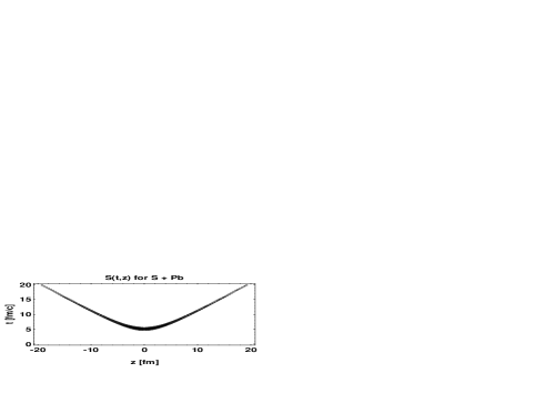
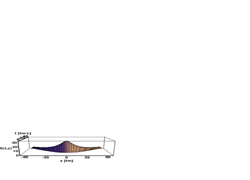
Figure 2: Contour plot of the reconstructed source function for $S+Pb$ reactions as measured by the NA44 collaboration. Note the large value of the mean freeze-out time and the narrow width of the emission zone in proper-time.

Figure 3: Parametric plot of the reconstructed source function for $S+Pb$ reactions as measured by the NA44 collaboration. The source is the same as that of Figure 2, but a different view-point is chosen to show the shape of emission probabilities for large values of $|z|$ in the mid-rapidity frame.

On Figures 2 and 3 we indicate the reconstructed space-time distribution of the source of particles in 200 AGeV central $S+Pb$ reactions, as a function of the time variable $t$ and the coordinate along the beam direction, $z$, both measured in the mid-rapidity frame that moves in the laboratory with $y_{0}=3.0$. The momentum-integrated emission function at $r_{x}=r_{y}=0$ is given by

$$S_{c}(t,z)\propto\exp\left(-{(\tau-\tau_{0})^{2}\over 2\Delta\tau^{2}}\right)\,\,\exp\left(-{(\eta-y_{0})^{2}\over 2\Delta\eta^{2}}\right)$$ (11)

where the parameters are taken from Table 1, corresponding to the best fit to NA44 $S+Pb$ data in this picture. Note the relation $(t,z)=(\tau\cosh(\eta),\tau\sinh(\eta))$. The contour-plot of $S_{c}(t,z)$ on Figure 2 shows that the with of particle emission is found to be narrow in proper-time. The parametric plot of $S_{c}(t,z)$ on Figure 3 indicates the long tails of particle production in the $|z|\approx t$ regions, the height of the curve is proportional to the production probability.

Note that in our case the hypothesis that pions, kaons and protons are emitted from the same hydrodynamical source is in a good agreement with the fitted data. The hypothesis that pion and kaons are emitted from different sources was investigated in ref. $\!{}^{{\bf?}}$, and this hypothesis resulted in a worse description of the data than the hypothesis that the pions and kaons are produced from the same source.

4.2 Comparision to hadron - proton reactions at CERN SPS

The NA22 collaboration fitted the same model to 250 GeV meson + p data $\!{}^{{\bf?}}$. Their best fit parameter values were $\Delta\eta=1.36\pm 0.02$, $T_{0}=140\pm 3$ MeV, $\langle u_{t}\rangle=0.20\pm 0.07$ and $\langle{\Delta T\over T}\rangle_{r}=0.71\pm 0.14$. From a combined HBT and spectrum analysis the NA22 experiment finds a mean freeze-out time of $\tau_{0}=1.4\pm 0.1$ fm/c, and a comparable duration parameter $\Delta\tau\geq\Delta\tau_{*}=1.3\pm 0.3$ fm/c. The transverse geometrical radius was found to be $R_{G}=0.88\pm 0.13fm$, which is slightly larger than the corresponding Gaussian radius parameter of the proton.

When comparing the source parameters of $S+Pb$ reactions to $h+p$ we find that the freeze-out temperature at the mean emission time at the center is similar in both cases. The surface temperatures are also equal within errors ($82\pm 7$ MeV vs. $107\pm 28\pm 18$ MeV). The width of the particle emission in spacetime-rapidity $\eta$ is also similar, $1.36\pm 0.02$ vs. $1.6\pm 0.3\pm 0.3$. However, we find a significantly larger mean freeze-out time in $S+Pb$ reactions as compared to $h+p$ reactions ($5.1\pm 0.3\pm 0.3$ fm/c vs. $1.4\pm 0.1$ fm/c). It seems that we observe a sharper freeze-out hypersurface in heavy ion collisions than in hadron-proton reactions, cf. $\Delta\tau=0.3\pm 0.3\pm 0.3$ vs. $\Delta\tau\geq 1.3\pm 0.3$ fm/c. The transversal radius of the matter is also larger in $S+Pb$ reactions, $5.4\pm 0.9\pm 0.7$ vs. $0.88\pm 0.13$ fm. We also find a much stronger transverse flow in $S+Pb$ than $h+p$ reactions.

4.3 Comparision to other NA44 data

A comparision of this analysis of NA44 data for $S+Pb$ reactions to recent NA44 results $\!{}^{{\bf?}}$ on $p+p$, $S+S$ and $Pb+Pb$ reactions shows that the freeze-out temperature in the center at the mean freeze-out time, $T_{0}$, in our case of $S+Pb$ reactions is within errors similar to the values obtained from an analysis of the particle spectra of $p+p$, $S+S$ and $Pb+Pb$ reactions $\!{}^{{\bf?}}$. In the $S+Pb$ case, we have a complete description, including the low $p_{t}$ part of the pion spectra with an acceptible $\chi^{2}/ndf$ due to our inclusion of the temperature inhomogeneities. Note also that we do not simply reproduce the slopes of particle spectra but we reproduce the absolute normalized particle spectra for pions, kaons, as well as the full shape of the proton spectra and the HBT radii.

5 Conclusions

A combined fitting of HBT radius parameters and spectrum fitting is presented in the Buda-Lund hydrodynamical parameterization scheme for CERN SPS heavy ion reactions.

It was necessary to use different particles and absolutely normalized particle spectra to obtain a well-defined minimum of each parameters for data from the small NA44 acceptance. The model is shown to describe the data in a statistically acceptable manner. The parameters can be determined with an accuracy of 10 - 20 % relative errors including systematic uncertainties. The transverse flow and the radial temperature inhomogeneity is necessary to achieve this result.

The same model describes meson - p spectra and correlations at CERN SPS with a similar central temperature, similar surface temperature and similar space-time rapidity width. The main difference between $S+Pb$ and $(\pi/K)+p$ reactions is that the geometrical radii, the freeze-out time and the transverse flow are much larger in the first case. The particle emission seems to happen more suddenly in S + Pb as compared to hadron induced reactions at the same energy range.

References

References

- [1] Proceedings of the Quark Matter conferences, Nucl. Phys. A 610, (1996); Nucl. Phys. A 590, (1995).
- [2] L. Lönnblad and T. Sjöstrand, Phys. Lett. B 351, 293-301 (1995).
- [3] T. Csörgő and B. Lörstad, hep-ph/9509213; Phys. Rev. C 54, 1390 (1996).
- [4] T. Csörgő and B. Lörstad, Nucl. Phys. A 590, 465 (1995).
- [5] H. Beker et al., NA44 Collaboration, Phys. Rev. Lett. 74, 3340 (1995).
- [6] N. M. Agababyan et al, NA22 Collaboration, Z. Phys. C 71, 405 (1996).
- [7] B. Lörstad and O. Smirnova, DELPHI Collaboration, Proceedings of the Correlations and Fluctuations’96 conference, Nijmegen, The Netherlands, June 1996, (World Scientific, Singapore, eds R. C. Hwa, W. Kittel et al.), p. 42.
- [8] T. Csörgő, Phys. Lett. B 347, 354 (1995).
- [9] T. Csörgő, P. Lévai and B. Lörstad, Acta Phys. Slovaka 46, 585 (1996).
- [10] N. M. Agababyan et al, NA22 Collaboration, preprint HEN-405 (1997); submitted to Phys. Lett. B
- [11] J. Bolz et al, Phys. Rev. D 47, 3860 (1993).
- [12] T. Csörgő, B. Lörstad and J. Zimányi, Z. Phys. C 71, 491 (1996).
- [13] T. Csörgő, Phys. Lett. B 409, 11 (1997).
- [14] T. Csörgő and B. Lörstad, Heavy Ion Physics 4, 221 (1996).
- [15] M. Murray, NA44 Collaboration, private communication.
- [16] S. Chapman, P. Scotto and U. Heinz, Heavy Ion Physics 1, 1 (1995); Phys. Rev. Lett. 74, 4400 (1995).
- [17] I. G. Bearden et al, NA44 Collaboration, Phys. Rev. Lett. 78, 2080 (1997).