Gravitational Phase Transition of Fermionic Matter in a General-Relativistic Framework

Abstract

The Thomas-Fermi model at finite temperature is extended to describe a system of self-gravitating weakly interacting massive fermions in a general-relativistic framework. The existence and properties of the gravitational phase transition in this model are investigated numerically. It is shown that, by cooling a nondegenerate gas of weakly interacting massive fermions below some critical temperature, a condensed phase emerges, consisting of quasidegenerate fermion stars. For fermion masses of 10 to 25 keV, these fermion stars may very well provide an alternative explanation for the supermassive compact dark objects that are observed at galactic centers.

1 Introduction

The ground state of a condensed cloud of fermionic matter, interacting only gravitationally and having a mass $M$ below the Oppenheimer-Volkoff (OV) limit [1], is a cold fermion star in which the degeneracy pressure balances the gravitational attraction of the fermions. Degenerate stars of fermions in the mass range between 10 and 25 keV are particularly interesting [2], as they could explain, without resorting to the black-hole hypothesis, at least some of the features observed around the supermassive compact dark objects with masses in the range of $M=10^{6.5}$ to $10^{9.5}$ solar masses, that are reported to exist at the centers of a number of galaxies [3, 4, 5, 6, 7, 8], including our own [9, 10], and quasistellar objects (QSO) [11, 12, 13, 14]. Indeed, there is little difference between a supermassive black hole and a fermion star of the same mass near the OV limit, a few Schwarzschild radii away from the object [15, 16].

The purpose of this paper is to study, in the framework of a general-relativistic Thomas-Fermi model, the formation of such a star that could have taken place in the early universe shortly after the nonrelativistic fermionic matter began to dominate the radiation. This system was previously studied in the Newtonian approximation [17, 18, 19, 20, 21, 22], and it was shown that the canonical and grand-canonical ensembles for such a system have a nontrivial thermodynamical limit [17, 18, 19]. Under certain conditions these systems will undergo a phase transition that is accompanied by a gravitational collapse [21, 22]. The phase transition occurs uniquely in the case of the attractive gravitational interaction of neutral fermions. As the phase transition does not happen for particles obeying Bose-Einstein or Boltzmann statistics, this phenomenon is quite distinct from the usual gravitational clustering of collisionless dark-matter particles. Gravitational condensation will also take place if the fermions have an additional short-range weak interaction, as neutrinos, neutralinos, gravitinos, and other weakly interacting massive particles do.

Effects of general relativity cannot be neglected when the total mass of the system is close to the OV limit [1]. There are three main features that distinguish the general-relativistic Thomas-Fermi model from the Newtonian one: i) the equation of state is relativistic, ii) the temperature and chemical potential are metric-dependent local quantities, and iii) the gravitational potential satisfies Einstein’s field equations instead of Poisson’s equation.

This paper is organized as follows: In Section 2 we briefly discuss the nonrelativistic Thomas-Fermi model at finite temperature. In Section 3 this model is extended within a general-relativistic framework. In Section 4 we discuss the solution at zero and finite temperature and, in particular, the conditions under which the first-order gravitational phase transition occurs. Conclusions are drawn in Section 5 and, finally, in Appendix A, we prove a theorem on the extremal properties of the free energy.

2 Thomas-Fermi model in Newtonian gravity

Consider a system of $N$ fermions of mass $m$ interacting only gravitationally, confined in a spherical cavity of radius $R$, in equilibrium at a finite temperature $T$. For large $N$, we can assume that the fermions move in a spherically symmetric mean-field potential $V(r)$ which satisfies Poisson’s equation

$$\frac{1}{r}\frac{d^{2}}{dr^{2}}(rV)=4\pi Gm^{2}n,$$ (2.1)

$G$ being the gravitational constant. The number density of the fermions (including antifermions) $n$ can be expressed in terms of the Fermi-Dirac distribution (in units $\hbar=c=k=1$)

$$n(r)=g\int\frac{d^{3}q}{(2\pi)^{3}}\left[1+\exp\left(\frac{q^{2}}{2mT}+\frac{V(r)}{T}-\frac{\mu}{T}\right)\right]^{-1}.$$ (2.2)

Here $g$ denotes the combined spin-degeneracy factors of the neutral fermions and antifermions, i.e., $g$ is 2 or 4 for Majorana or Dirac fermions, respectively. For each solution $V(r)$ of Eq. (2.1), the chemical potential $\mu$ is adjusted so that the constraint

$$\int d^{3}rn(r)=N$$ (2.3)

is satisfied. It may be shown that a particular spherically symmetric configuration $\bar{n}(r)$ will satisfy Eqs. (2.1)-(2.3) if and only if it extremizes the free energy functional defined as [18]

$$F[n]\! \!=\! \!\mu[n]N-\frac{1}{2}\int d^{3}rn(r)V[n]$$ (2.4)

$$-Tg\int\frac{d^{3}rd^{3}q}{(2\pi)^{3}}\ln\left(1+\exp\left(-\frac{q^{2}}{2mT}-\frac{V[n]}{T}+\frac{\mu[n]}{T}\right)\right),$$

where $V[n]$ and $\mu[n]$ are implicit functionals of $n(r)$ through Eqs. (2.1)-(2.3). For a physical solution, we have to require that the free energy is minimal, i.e.,

$$\left.\frac{\delta F}{\delta n}\right|_{\bar{n}}=0,\;\;\;\;\left.\frac{\delta^{2}F}{\delta n^{2}}\right|_{\bar{n}}\geq 0.$$ (2.5)

The set of self-consistency equations (2.1)-(2.3), together with (2.5), comprises the nonrelativistic gravitational Thomas-Fermi model.

It may be easily shown that the following scaling property holds: If the potential energy $V(r)$ is a solution to the self-consistency equations (2.1)-(2.3), then the rescaled $\tilde{V}=A^{4}V(Ar)$, with $A>0$, is also a solution with the rescaled fermion number $\tilde{N}=A^{3}N$, radius $\tilde{R}=A^{-1}R$, and temperature $\tilde{T}=A^{4}T$. This property, which will be referred to as nonrelativistic scaling, implies the existence of a thermodynamic limit of $N^{-7/3}F$, with $N^{1/3}R$ and $N^{-4/3}T$ approaching constant values for $N\rightarrow\infty$. In this limit, the Thomas-Fermi equation becomes exact [18, 19].

3 Thomas-Fermi model in general relativity

Consider a self-gravitating gas consisting of $N$ fermions of mass $m$ in equilibrium within a sphere of radius $R$. We denote by $p$, $\rho$, $n$, and $\sigma$ the pressure, energy density, particle number density, and entropy density of the gas, respectively. The metric generated by the mass distribution is static, spherically symmetric, and asymptotically flat, i.e.,

$$ds^{2}=\xi^{2}dt^{2}-(1-2{\cal{M}}/r)^{-1}dr^{2}-r^{2}(d\theta^{2}+\sin\theta d\phi^{2}).$$ (3.1)

Einstein’s field equations are then given by

$$\frac{d\xi}{dr}=\xi\frac{{\cal M}+4\pi r^{3}p}{r(r-2{\cal{M}})}\,,$$ (3.2)

$$\frac{d{\cal{M}}}{dr}=4\pi r^{2}\rho,$$ (3.3)

with the boundary conditions

$$\xi(R)=\left(1-\frac{2{\cal{M}}(R)}{R}\right)^{1/2}\,;\;\;\;\;\;{\cal{M}}(0)=0.$$ (3.4)

The equation of state may be represented in a parametric form [23]

$$n=g\int\frac{d^{3}q}{(2\pi)^{3}}\,\frac{1}{1+e^{E/\bar{T}-\bar{\mu}/\bar{T}}}\,,$$ (3.5)

$$\rho=g\int\frac{d^{3}q}{(2\pi)^{3}}\,\frac{E}{1+e^{E/\bar{T}-\bar{\mu}/\bar{T}}}\,,$$ (3.6)

$$p=g\bar{T}\int\frac{d^{3}q}{(2\pi)^{3}}\,\ln(1+e^{-E/\bar{T}+\bar{\mu}/\bar{T}})\,,$$ (3.7)

where $g$ denotes the spin degeneracy factor and $E=\sqrt{m^{2}+q^{2}}$. The quantities $\bar{T}$ and $\bar{\mu}$ are the local temperature and chemical potential, respectively. As discussed in Appendix A, thermodynamic and hydrostatic equilibrium in the presence of gravity implies

$$\bar{T}(r)=\frac{T}{\xi(r)}\,;\;\;\;\;\;\;\bar{\mu}(r)=\frac{\mu}{\xi(r)}\,.$$ (3.8)

The constants $T$ and $\mu$ are the temperature and chemical potential at infinity. Although the matter is absent at $r=\infty$, the temperature at infinity has a physical meaning: T is the ”red shifted” temperature [24] of the black-body radiation of a gravitating object in equilibrium at finite temperature measured at infinity. In other words, our gravitating object is in equilibrium with a heat bath which could be thought of as a black-body radiation in the empty space surrounding the object. As a consequence of Eq. (3.8), different gravitating configurations of the same size “in contact” with the same heat bath may have different surface temperatures. Therefore, the relevant equilibrium parameter is the temperature of the heat bath, $T$, and not the surface temperature of the gravitating object. Particle number conservation yields the constraint

$$\int_{0}^{R}dr\,4\pi r^{2}(1-2{\cal{M}}/r)^{-1/2}\,n(r)=N.$$ (3.9)

Given the temperature at infinity $T$, the set of self-consistency equations (3.2)-(3.9) defines the general-relativistic Thomas-Fermi equation. One additional important requirement is that a solution to the equations (3.2)-(3.9) should minimize the free energy. Based on the considerations given in Appendix A, the free energy may be written in the form

$$F=M+\mu N-\int dr4\pi r^{2}\xi(1-2{\cal{M}}/r)^{-1/2}(p+\rho),$$ (3.10)

with $M={\cal M}(R)$. The theorem proved in Appendix A guarantees that solutions to Eqs. (3.2)-(3.9) extremize the free energy $F$, i.e., the free-energy functional assumes either a maximum or a minimum. We only have to find out which of the solutions are maxima and discard them as unphysical.

Next we show that, in the Newtonian limit, we recover the usual Thomas-Fermi model as defined in Section 2. Introducing the nonrelativistic chemical potential $\mu_{NR}=\mu-m$ and the approximations $\xi=e^{\varphi}\simeq 1+\varphi$, $E\simeq m+q^{2}/2m$ and ${\cal M}/r\ll 1$ , we arrive at the Thomas-Fermi self-consistency equations [21, 22] in the form

$$n=\frac{\rho}{m}=g\int\frac{d^{3}q}{(2\pi)^{3}}\,\left(1+\exp(\frac{q^{2}}{2mT}+\frac{m}{T}\varphi-\frac{\mu_{NR}}{T})\right)^{-1}\,,$$ (3.11)

$$\frac{d\varphi}{dr}=\frac{{\cal M}}{r^{2}}\,;\;\;\;\;\frac{d{\cal{M}}}{dr}=4\pi r^{2}\rho\,,$$ (3.12)

$$\varphi(R)=-\frac{mN}{R}\,;\;\;\;{\cal{M}}(0)=0,$$ (3.13)

$$\int_{0}^{R}dr\,4\pi r^{2}n(r)=N,$$ (3.14)

which are equivalent to the set of equations (2.1)-(2.3). The free energy (3.10) in the Newtonian limit yields

$$F=mN+\mu_{NR}N-\frac{1}{2}\int_{0}^{R}dr\,4\pi r^{2}n\varphi-\int_{0}^{R}dr\,4\pi r^{2}p\,,$$ (3.15)

with

$$p=gT\int\frac{d^{3}q}{(2\pi)^{3}}\,\ln\left(1+\exp(-\frac{q^{2}}{2mT}-\frac{m}{T}\varphi+\frac{\mu_{NR}}{T})\right)\,,$$ (3.16)

which, up to a constant, is equal the nonrelativistic Thomas-Fermi free energy (2.4).

A straightforward thermodynamic limit $N\rightarrow\infty$, as discussed by Hertel, Thirring, and Narnhofer [18, 19], is not directly applicable in the general-relativistic case. First, in contrast to the Newtonian case, there exists a limiting configuration with maximal $M$ and $N$ (the OV limit) at zero temperature, and, as we shall shortly demonstrate, also at finite temperature. Second, the scaling property of the relativistic Thomas-Fermi equation, which will be referred to as relativistic scaling, is quite distinct from nonrelativistic scaling. This scaling property may be formulated as follows: If the configuration $\{\xi(r),{\cal{M}}(r)\}$ is a solution to the self-consistency equations (3.2)-(3.9), then the configuration $\{\tilde{\xi}=\xi(A^{-1}r),\tilde{\cal M}=A{\cal{M}}(A^{-1}r);A>0\}$ is also a solution with the rescaled fermion number $\tilde{N}=A^{3/2}N$, radius $\tilde{R}=AR$, asymptotic temperature $\tilde{T}=A^{-1/2}T$, and fermion mass $\tilde{m}=A^{-1/2}m$. The free energy is then rescaled as $\tilde{F}=AF$. Hence, there exists a thermodynamic limit of $N^{-2/3}F$, with $N^{-2/3}R$, $N^{1/3}T$, and $N^{1/3}m$ approaching constant values when $N\rightarrow\infty$.

4 Numerical integration

In the following we use the units in which $G=1$. We choose appropriate length, mass and fermion number scales $a$, $b$, and $c$ respectively, such that

$$a=b=\sqrt{\frac{2}{g}}\,\frac{1}{m^{2}},\;\;\;\;c=\frac{b}{m},$$ (4.1)

or, restoring $\hbar$, $c$, and $G$, we have

$$a=\sqrt{\frac{2}{g}}\,\frac{\hbar M_{\rm{Pl}}}{cm^{2}}=1.3185\times 10^{10}\,\sqrt{\frac{2}{g}}\,\left(\frac{15{\rm keV}}{m}\right)^{2}{\rm km},$$ (4.2)

$$b=\sqrt{\frac{2}{g}}\,\frac{M_{\rm{Pl}}^{3}}{m^{2}}=0.8929\times 10^{10}\,\sqrt{\frac{2}{g}}\,\left(\frac{15{\rm keV}}{m}\right)^{2}M_{\odot}$$ (4.3)

$$c=\sqrt{\frac{2}{g}}\,\frac{M_{\rm{Pl}}^{3}}{m^{3}}=5.5942\times 10^{71}\,\sqrt{\frac{2}{g}}\,\left(\frac{15{\rm keV}}{m}\right)^{3}$$ (4.4)

where $M_{\rm{Pl}}=\sqrt{\hbar c/G}$ denotes the Planck and $M_{\odot}$ the solar mass.

We are looking for a solution of the Thomas-Fermi problem as a function of temperature. For numerical convenience, let us introduce a new parameter

$$\alpha=\frac{\mu}{T}$$ (4.5)

and the substitution

$$\xi=\frac{\mu}{m}(\Phi+1)^{-1/2}.$$ (4.6)

Using this and (4.1), Eqs. (3.5)-(3.7) may be written in the form

$$n=\frac{1}{\pi^{2}}\int^{\infty}_{0}dy\,\frac{y^{2}}{1+\exp[(\sqrt{(y^{2}+1)/(\Phi+1)}-1)\alpha]}\,,$$ (4.7)

$$\rho=\frac{1}{\pi^{2}}\int^{\infty}_{0}dy\,\frac{y^{2}\sqrt{y^{2}+1}}{1+\exp[(\sqrt{(y^{2}+1)/(\Phi+1)}-1)\alpha]}\,,$$ (4.8)

$$p=\frac{1}{3\pi^{2}}\int^{\infty}_{0}dy\,\frac{y^{4}}{\sqrt{y^{2}+1}(1+\exp[(\sqrt{(y^{2}+1)/(\Phi+1)}-1)\alpha]}\,.$$ (4.9)

In this way, both the fermion mass and the chemical potential are eliminated from the equation of state.

The field equations (3.2) and (3.3) now read

$$\frac{d\Phi}{dr}=-2(\Phi+1)\frac{{\cal M}+4\pi r^{3}p}{r(r-2{\cal{M}})}\,,$$ (4.10)

$$\frac{d{\cal{M}}}{dr}=4\pi r^{2}\rho.$$ (4.11)

To these two equations we add

$$\frac{d{\cal N}}{dr}=4\pi r^{2}(1-2{\cal{M}}/r)^{-1/2}n$$ (4.12)

imposing the particle-number constraint as a condition at the boundary

$${\cal N}(R)=N.$$ (4.13)

Equations (4.10)-(4.12) should be integrated using the boundary conditions at the origin

$$\Phi(0)=\Phi_{0}>-1\,;\;\;\;\;\;{\cal{M}}(0)=0;\,;\;\;\;\;\;{\cal{N}}(0)=0.$$ (4.14)

The parameter $\Phi_{0}$, which is uniquely related to the central density and pressure, will eventually be fixed by the requirement (4.13). For $r\geq R$, the function $\Phi$ yields the usual empty-space Schwarzschild solution

$$\Phi(r)=\frac{\mu^{2}}{m^{2}}\left(1-\frac{2M}{r}\right)^{-1}-1\,,$$ (4.15)

with

$$M={\cal M}(R)=\int_{0}^{R}dr4\pi r^{2}\rho(r).$$ (4.16)

We now show that a solution to the general-relativistic Thomas-Fermi equation exists provided the number of fermions is smaller than a certain number $N_{\rm max}$ that depends on $\alpha$ and $R$. From (4.8) and (4.9) it follows that, for any $\alpha>0$, the equation of state $\rho(p)$ is an infinitely smooth function and $d\rho/dp>0$ for $p>0$. Then, as shown by Rendall and Schmidt [25], there exists for any value of the central density $\rho_{0}$ a unique static, spherically symmetric solution of the field equations with $\rho\rightarrow 0$ as $r$ tends to infinity. In that limit ${\cal M}(r)\rightarrow\infty$ and ${\cal N}(r)\rightarrow\infty$, as may be easily seen by analyzing the $r\rightarrow\infty$ limit of Eqs. (4.10) and (4.11). However, the enclosed mass $M$ and the number of fermions $N$ within a given radius $R$ will be finite. We can then cut off the matter from $R$ to infinity and join the interior solution onto the empty space Schwarzschild exterior solution by making use of equation (4.15). This equation together with (4.5) fixes the chemical potential and the temperature at infinity. Furthermore, it may be shown that our equation of state obeys asymptotically at high densities a $\gamma$-law, i.e., $\rho=$ const $n^{\gamma}$ and $p=(\gamma-1)\rho$, with $\gamma=4/3$. In this case, as is well known [26], there exists a limiting configuration $\{\psi_{\infty}(r),{\cal{M}}(r)_{\infty}\}$ such that $M$ and $N$ approach nonzero values $M_{\infty}$ and $N_{\infty}$, respectively, as the central density $\rho_{0}$ tends to infinity. Thus, the quantity $N$ is a continuous function of $\rho_{0}$ on the interval $0\leq\rho_{0}<\infty$, with $N=0$ for $\rho_{0}=0$, and $N=N_{\infty}$ as $\rho_{0}\rightarrow\infty$. The range of $N$ depends on $\alpha$ and $R$ and its upper bound may be denoted by $N_{\rm max}(R,\alpha)$. Thus, for given $\alpha$, $R$ and $N<N_{\rm max}(R,\alpha)$ the set of self-consistency equations (4.7)-(4.16) has at least one solution.

As is evident from the equation of state (3.5)-(3.7), if we do not fix the boundary and do not constrain the particle number $N$, the pressure (and the density) will never vanish (except perhaps at $r=\infty$), unless $T=0$. Thus, since we fix the boundary at $R$ and cut off the matter from $R$ to infinity, the pressure (and the density) will have a discontinuity. This characteristic of the non-relativistic Thomas-Fermi model in atomic physics [27], and Newtonian gravity [18, 21, 22] remains also in general relativity. However, the density and the pressure decrease rapidly with $r$, so if $R$ is chosen sufficiently large, the pressure and the density at the boundary will be extremely small. Furthermore, the region $r>R$ is never empty in reality, so that a positive pressure at the boundary is more realistic than a vanishing pressure.

The numerical procedure is now straightforward. For a fixed, arbitrarily chosen $\alpha$, we first integrate equations (4.10) and (4.11) numerically on the interval $(0,R)$ and find solutions for various initial $\Phi_{0}$. Simultaneously integrating (4.12), we obtain ${\cal N}(R)$ as a function of $\Phi_{0}$. The specific value of $\Phi_{0}$ is then determined such that ${\cal N}(R)=N$. The chemical potential $\mu$ corresponding to this particular solution is given by (4.15). If we now eliminate $\mu$ using (4.5), we finally get the parametric dependence on temperature through $\alpha$.

Let us first discuss a degenerate fermion gas ($T=0$) as a reference point that can also be compared with the well-known results by Oppenheimer and Volkoff [1]. In this case, the Fermi distribution in (4.7)-(4.9) becomes a step function that yields an elementary integral with the upper limit $y_{F}=\sqrt{\Phi}$ related to the Fermi momentum

$$q_{F}=m\sqrt{\Phi}.$$ (4.17)

The equation of state can be expressed in terms of elementary functions of $\Phi$

$$n=\frac{1}{3\pi^{2}}\Phi\sqrt{\Phi},$$ (4.18)

$$\rho=\frac{1}{8\pi^{2}}\left[(2\Phi+1)\sqrt{\Phi(\Phi+1)}-{\rm Arsh}\sqrt{\Phi}\right],$$ (4.19)

$$p=\frac{1}{24\pi^{2}}\left[(2\Phi-3)\sqrt{\Phi(\Phi+1)}+3{\rm Arsh}\sqrt{\Phi}\right].$$ (4.20)

The radius of the star is naturally defined as the point where the density vanishes. At this point, owing to (4.18), $\Phi=0$. Therefore, we integrate equations (4.7)-(4.9) starting from $r=0$ up to the point $R$ where $\Phi(R)=0$. As a result, the quantities $M$, $N$, and $R$ are obtained as functions of the parameter $\Phi_{0}$, which is related to the central particle-number density through (4.18). In Fig. 1, we plot the mass of the star as a function of the radius $R$. The maximum of the curve corresponds to the OV limit [1]. The limiting values are $R_{\rm OV}=3.357$, $M_{\rm OV}=0.38426$, and $N_{\rm OV}=0.39853$, in units of $a$, $b$, and $b/m$ respectively. The curve left from the maximum represents unstable configurations that curl up around the point corresponding to the infinite central density limit.

Figure 1: Mass versus radius for fermion stars at zero temperature in the general-relativistic framework (solid line) compared with the corresponding Newtonian approximation (dotted line). Dashed line is the black hole limit $M=R/2$.

We now turn to the study of nonzero temperature. The quantities $T$, $N$, and, $R$ are free parameters in our model and their range and choice are dictated by physics. The temperature $T$ is restricted only to positive values. The number of fermions $N$ is restricted by the Oppenheimer-Volkoff limit. The radius $R$ is theoretically unlimited; practically, it should not exceed the order of interstellar distances. It is known that a classical, semidegenerate, isothermal configuration has no natural boundary in contrast to the degenerate case of zero temperature, where for given $N$ (up to the Oppenheimer-Volkoff limit) the radius $R$ is naturally fixed by the condition of vanishing pressure and density. At nonzero temperature, if we, e.g., fix only $N$ and $T$ and let $R\rightarrow\infty$, our gas will occupy the entire space, and hence $p$ and $\rho$ will vanish everywhere. If we do not restrict $N$ and integrate the equations on the interval $(0,\infty)$, $M$ and $N$ will diverge at $\infty$. In such a case one has to introduce a cutoff. In the isothermal model of a similar kind by Chau, Lake, and Stone [30], a cutoff was chosen at the radius $R$, where the energy density was about six orders smaller than the central value. Our choice is based on the following considerations: As in the Newtonian Thomas-Fermi model [22], we expect that, for given number of fermions $N<N_{\rm OV}$, there exists a unique configuration that is a solution to the self-consistency equations (3.5) to (3.9) and which becomes a degenerate Fermi gas at $T=0$. For such a configuration, an effective radius $R_{\rm eff}\geq R_{\rm OV}$ may be defined so that $\Phi(R_{\rm eff})=0$. Although the density does not vanish at this point, most of the mass will be contained inside the sphere of radius $R_{\rm eff}$. If we choose the boundary at $R\gg R_{\rm OV}$, the total mass will be dominated by the density distribution within $R_{\rm eff}$, and it will be almost independent of the choice of $R$. Thus, in the following we will work with $R=100\simeq 30R_{\rm OV}$.

In Fig. 2, the fermion number $N$ is plotted as a function of initial $\Phi_{0}$ for several values of the parameter $\alpha$. In contrast to the $T=0$ case, all curves with finite $\alpha$ have a peak around $\Phi=0$. The second peak corresponds to the OV limit. From this figure we can deduce that, for a given $N$, there is a range of $\alpha$’s for which the Thomas-Fermi equation may have more than one solution. This is a clear indication for the existence of an instability even below the OV limit and, as a consequence, we expect that a first-order phase transition occurs.

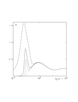
Figure 2: Fermion number $N$versus central potential $\Phi_{0}$ for $\alpha=\frac{\mu}{T}=300$ (full line) 500 (dashed line) and 150 (dot-dashed line). T=0 is represented by dotted line.

Figure 3: Temperature T (in units of $m$) versus $1/\alpha$ for $N=0.38$ and $R=100$.

Fixing $N=0.38$, which is slightly below the OV limit, we can now plot the temperature as a function of $\alpha$ in Fig. 3. Using this figure as a parametric function for temperature, the mass, free energy, and entropy are shown as functions of temperature in Figs. 4, 5, and 6, respectively. In the temperature interval $T=(0.0015-0.007)m$ there are three distinct solutions of which only two are physical, namely, those for which the free energy assumes a minimum. The solution that can be continuously extended to any temperature above the mentioned interval is referred to as “gas”, whereas the solution that continues to exist at low temperatures, and eventually becomes a degenerate Fermi gas at $T=0$, will be called “condensate”. In Fig. 2 the gas is represented on each curve by the part left from the first maximum, while the part from the first minimum up to the second maximum represents the condensate. By noting that $\Phi_{0}$ is negative for the gas and positive for the condensate, we may define an order parameter as

$$\delta=\Phi_{0}+|\Phi_{0}|,$$ (4.21)

which is strictly positive in the condensed phase (ordered phase) and equal to zero in the gaseous phase (disordered phase).

Figure 4: Total mass (in units of $b$) versus temperature for $N=0.38$ and $R=100$.

Figure 5: Free energy per fermion $F/N$ (in units of $m$) versus temperature T for $N=0.38$ and $R=100$.

Figure 6: Entropy per fermion $S/N$ versus temperature $T$ for $N=0.38$ and $R=100$.

The phase transition takes place at the temperature $T_{c}$, where the free energy of the gas and that of the condensate become equal. The dashed curves in Figs. 4, 5, and 6 represent the physically unstable solution. In our example, the transition temperature is $T_{c}=0.0043951m$, as indicated in the plots by the dotted line. The latent heat per fermion released during the phase transition is given by the mass difference at the point of discontinuity

$$\frac{\Delta M}{N}=0.0438m.$$ (4.22)

So far, we have studied, as an example, an object with number of fermions $N$ just below the OV limit $N_{\rm OV}$. Any object with $N<N_{\rm OV}$ will undergo a gravitational phase transition at a critical temperature which depends on the mass, of course. With decreasing $N$, the cavity radius $R$ must be appropriately increased, since the effective radius of the condensate increases following approximately the zero-temperature mass-radius relation. As $N$ becomes smaller, the system approaches the nonrelativistic scaling regime discussed in Sec. 2, and for $N\ll N_{\rm OV}$ the critical temperature will decrease according to

$$T_{c}={\rm const}\,N^{4/3},$$ (4.23)

if the cavity radius $R$ is simultaneously rescaled as $N^{-1/3}$. In Fig. 7 we compare the critical temperature calculated in both Newtonian and general-relativistic Thomas-Fermi models, as a function of $N$. The nonrelativistic scaling law turns out to be very accurate for $N<0.2\,N_{\rm OV}$.

Figure 7: Critical temperature as a function of the fermion number in the Newtonian (dashed line) and general-relativistic Thomas-Fermi model (solid line).

It is important to check that the critical temperature is not very sensitive to variations of the cavity radius $R$ for the following two reasons: First, in our model $R$ is arbitrary except for the requirement that it should be much larger then the effective radius which for $N=0.38$ is of the order $R_{\rm eff}\simeq R_{\rm OV}=3.357$. Second, if the critical temperature rapidly decreases with $R$, the adiabatic cooling of the gas through the universe expansion may not necessarily lead to the point of the phase transition. Fig. 8 shows that the critical temperature indeed decreases very slowly, roughly by a factor of two if $R$ increases from 30 to 300. This is much weaker than the adiabatic cooling of a nonrelativistic gas which goes approximately as $1/R^{2}$. Thus we conclude that the gravitational phase transition will necessarily take place in the course of the universe expansion.

Figure 8: Critical temperature $T_{c}$ as a function of the cavity radius $R$ for $N=0.38$.

5 Conclusions

In this work, we have extended the Thomas-Fermi model to a general-relativistic framework. This model was then applied to a system of self-gravitating fermions. We have investigated numerically the circumstances under which this system undergoes a gravitational phase transition at nonzero temperature. This phase transition is quite distinct from the more extensively investigated strong-interaction driven phase transition that might occur in neutron stars [28, 29]. The main underlying physics here is the competition between the partial degeneracy pressure due to the Fermi-Dirac statistics and the attractive force due to the gravitational interaction. It is obvious that the application of this model to astrophysical systems will work very well if the non-gravitational interactions between the individual particles can be neglected. This is certainly the case, e.g., for weakly interacting quasidegenerate heavy neutrino neutralino, or gravitino matter [15, 22, 30, 31, 32], but perhaps it could be valid even for collisionless stellar systems [33, 34].

Finally, let us briefly comment on a similar model by Chau, Lake and Stone [30] which was considered earlier in the context of a possible galactic massive neutrino halo. Their model differs from our approach in essentially two aspects: First, the equation of state is not consistent with the condition of thermodynamical and chemical equilibrium, i.e. with Eq. (3.8) and second, the particle number constraint (3.9) is not imposed. Thus, in contrast to the Thomas-Fermi model discussed here, the Chau et al. model does not describe a canonical system in equilibrium.

Acknowledgment

We acknowledge useful discussions with D. Tsiklauri. This work was supported by the Foundation for Fundamental Research (FFR).

Appendix A Free Energy

Consider a canonical ensemble that describes a nonrotating fluid in equilibrium at nonzero temperature. We denote by $u_{\mu}$ , $p$, $\rho$, $n$, and $\sigma$ the velocity, pressure, energy density, particle number density, and entropy density of the fluid. A canonical ensemble is subject to the constraint that the total number of particles

$$\int_{\Sigma}n\,u^{\mu}d\Sigma_{\mu}=N$$ (A.1)

should be fixed. The spacelike hypersurface $\Sigma$ that contains the fluid is orthogonal to the time-translation Killing vector field $k^{\mu}$ which is related to the velocity of the fluid by

$$k^{\mu}=\xi u^{\mu}\,;\;\;\;\;\;\;\xi=(k^{\mu}k_{\mu})^{1/2}.$$ (A.2)

The energy-momentum tensor is defined as

$$T_{\mu\nu}=(p+\rho)u_{\mu}u_{\nu}-pg_{\mu\nu}.$$ (A.3)

The metric generated by the mass distribution in equilibrium is static, spherically symmetric, and asymptotically flat, i.e.,

$$ds^{2}=\xi^{2}dt^{2}-\lambda^{2}dr^{2}-r^{2}(d\theta^{2}+\sin\theta d\phi^{2}).$$ (A.4)

The metric coefficients $\xi$ and $\lambda$ may be determined from Einstein’s field equations. However, we shall for the moment assume that $\xi$ is an arbitrary function of $r$, which asymptotically approaches unity, and we parameterize $\lambda$ in terms of the mass $\cal M$ within the radius $r$

$$\lambda=\left(1-\frac{2{\cal{M}}(r)}{r}\right)^{-1/2},$$ (A.5)

where

$${\cal{M}}(r)=\int^{r}_{0}dr^{\prime}\,4\pi r^{\prime 2}\rho(r^{\prime})\,.$$ (A.6)

The temperature $\bar{T}$ and chemical potential $\bar{\mu}$ are, in general, metric-dependent local quantities. The local law of energy-momentum conservation, $T^{\mu\nu}_{\;\;\;\;;\nu}=0$, for a perfect fluid in a static gravitational field, yields the equation of hydrostatic equilibrium [35]

$$\partial_{\nu}p=-(p+\rho)\xi^{-1}\partial_{\nu}\xi.$$ (A.7)

This equation, together with the thermodynamic identity (Gibbs-Duhem relation)

$$d\frac{\bar{\mu}}{\bar{T}}=\frac{1}{n}d\frac{p}{\bar{T}}+\frac{\rho}{n}d\frac{1}{\bar{T}},$$ (A.8)

and the condition that the heat flow and diffusion vanish

$$\frac{\bar{\mu}}{\bar{T}}={\rm const.},$$ (A.9)

implies

$$\bar{T}\xi=T\,;\;\;\;\;\;\;\bar{\mu}\xi=\mu\,,$$ (A.10)

where $T$ and $\mu$ are constants equal to the temperature and chemical potential at infinity. The temperature $T$ may be chosen arbitrarily as the temperature of the heatbath. The quantity $\mu$ in a canonical ensemble is an implicit functional of $\xi$ owing to the constraint (A.1). The first equation in (A.10) is the well known-Tolman condition for thermal equilibrium in a gravitational field [36].

Following Gibbons and Hawking [37], we postulate that the free energy of the canonical ensemble is

$$F=M-\int_{\Sigma}\bar{T}\sigma\,k^{\mu}d\Sigma_{\mu}\,,$$ (A.11)

where $M$ is the total mass as measured from infinity. The entropy density of a relativistic fluid may be expressed as

$$\sigma=\frac{1}{\bar{T}}(p+\rho-\bar{\mu}n),$$ (A.12)

$\bar{T}$ and $\bar{\mu}$ being the local temperature and chemical potential as defined in (A.10). Based on Eq. (A.10), the free energy may be written in the form analogous to ordinary thermodynamics

$$F=M-TS,$$ (A.13)

with $M={\cal{M}}(R)$, and the total entropy $S$ defined as

$$S=\int_{0}^{R}dr\,4\pi r^{2}\lambda\frac{1}{\bar{T}}(p+\rho)-\frac{\mu}{T}N,$$ (A.14)

where we have used spherical symmetry to replace the proper volume integral as

$$\int_{\Sigma}u^{\mu}d\Sigma_{\mu}=\int_{0}^{R}dr4\pi r^{2}\lambda.$$ (A.15)

The following theorem relates the extrema of the free energy with the solutions of Einstein’s field equation:

Theorem: Among all momentarily static, spherically symmetric configurations $\{\xi(r),{\cal{M}}(r)\}$ which, for a given temperature $T$ at infinity, contain a specified number of particles

$$\int_{0}^{R}4\pi r^{2}dr\,\lambda(r)n(r)=N$$ (A.16)

within a spherical volume of a given radius $R$, those and only those configurations that extremize the quantity F defined by (A.13) will satisfy Einstein’s field equation

$$\frac{d\xi}{dr}=\xi\frac{{\cal M}+4\pi r^{3}p}{r(r-2{\cal{M}})}\,,$$ (A.17)

with the boundary condition

$$\xi(R)=\left(1-\frac{2M}{R}\right)^{1/2}.$$ (A.18)

Proof: By making use of the identity (A.8) and the fact that $\delta(\bar{\mu}/\bar{T})=\delta(\mu/T)$ and that $N$ is fixed by the constraint (A.16), from Eqs. (A.13) and (A.14) we find

$$\delta F=\delta M-\int_{0}^{R}dr\,4\pi r^{2}\frac{T}{\bar{T}}(p+\rho)\delta\lambda-\int_{0}^{R}dr\,4\pi r^{2}\lambda\frac{T}{\bar{T}}\delta\rho\,.$$ (A.19)

The variations $\delta\lambda$ and $\delta\rho$ can be expressed in terms of the variation $\delta{\cal{M}}(r)$ and its derivative

$$\frac{d\delta{\cal M}}{dr}=4\pi r^{2}\delta\rho,$$ (A.20)

yielding

$$\delta F=\delta M-\int_{0}^{R}dr\,4\pi r^{2}\frac{T}{\bar{T}}(p+\rho)\frac{\partial\lambda}{\partial{\cal M}}\delta{\cal M}-\int_{0}^{R}dr\,\lambda\frac{T}{\bar{T}}\frac{\delta{\cal M}}{dr}\,.$$ (A.21)

By partial integration of the last term, and replacing $T/\bar{T}$ by $\xi$, we find

$$\delta F=\left[1-\lambda(R)\xi(R)\right]\delta M-\int_{0}^{R}dr\,\left[4\pi r^{2}\xi(p+\rho)\frac{\partial\lambda}{\partial{\cal M}}-\frac{d}{dr}(\lambda\xi)\right]\delta{\cal M}\,,$$ (A.22)

where $\delta{\cal{M}}(r)$ is an arbitrary variation on the interval $[0,R]$, except for the constraint $\delta{\cal{M}}(0)=0$. Therefore, $\delta F$ will vanish if and only if

$$4\pi r^{2}\xi(p+\rho)\frac{\partial\lambda}{\partial{\cal M}}-\frac{d}{dr}(\lambda\xi)=0$$ (A.23)

and

$$1-\lambda(R)\xi(R)=0.$$ (A.24)

Using Eqs. (A.5) and (A.6), we can write Eq. (A.23) in the form (A.17), and Eq. (A.24) gives the desired boundary condition (A.18). Thus, $\delta F=0$ if and only if a configuration $\{\xi,{\cal M}\}$ satisfies Eq. (A.17) with (A.18), as was to be shown.

Remark 1: A solution to Eq. (A.17) is dynamically stable if the free energy assumes a minimum.
Remark 2: Our Theorem 1 is a finite-temperature generalization of the result obtained for cold, catalyzed matter [26].

References

- [1] J.R. Oppenheimer and G.M. Volkoff, Phys. Rev. 55 (1939) 374.
- [2] R. D. Viollier, Prog. Part. Nucl. Phys. 32 (1994) 51.
- [3] J. L. Tonry, Astrophys. J. Lett. 283 (1984) 37; Astrophys. J. 322 (1987) 632.
- [4] A. Dressler, Astrophys. J. 286 (1994) 97.
- [5] A. Dressler and D. O. Richstone, Astrophys. J. 324 (1988) 701.
- [6] J. Kormendy, Astrophys. J. 325 (1988) 128.
- [7] J. Kormendy, Astrophys. J. 335 (1988) 40.
- [8] J. Kormendy and D. Richstone, Astrophys. J. 393 (1992) 559.
- [9] J. H. Lacy, C. H. Townes and D. J. Hollenbach, Astrophys. J. 262 (1982) 120.
- [10] J. H. Lacy, J. M. Achtermann and E. Serabyn, Astrophys. J. Lett. 380 (1991) 71.
- [11] D. Lynden-Bell, Nature 223 (1969) 690.
- [12] Ya. B. Zel’dovich and I. D. Novikov, “Stars and Relativity” in Relativistic Astrophysics, Vol.1 (U. of Chicago Press, Chicago, 1971).
- [13] R. D. Blandford and M. J. Rees, Mon. Not. R. Astron. Soc. 169 (1974) 395.
- [14] M. C. Begelman, R. D. Blandford and M. J. Rees, Rev. Mod. Phys. 56 (1984) 255.
- [15] N. Bilić, D. Tsiklauri, and R.D. Viollier, Prog. Part. Nucl. Phys. 40 (1998) 17.
- [16] D. Tsiklauri and R.D. Viollier, Astrophys. J. 500 (1998) 591.
- [17] W. Thirring, Z. Phys. 235 (1970) 339.
- [18] P. Hertel and W. Thirring, Comm. Math. Phys. 24 (1971) 22; P. Hertel and W. Thirring, “Thermodynamic Instability of a System of Gravitating Fermions”, in Quanten und Felder, edited by H. P. Dürr (Vieweg, Braunschweig, 1971).
- [19] P. Hertel, H. Narnhofer and W. Thirring, Comm. Math. Phys. 28 (1972) 159.
- [20] B. Baumgartner, Comm. Math. Phys. 48 (1976) 207.
- [21] J. Messer, J. Math. Phys. 22 (1981) 2910.
- [22] N. Bilić and R.D. Viollier, Phys. Lett. B 408 (1997) 75; N. Bilić and R.D. Viollier, Nucl. Phys. B (Proc. Suppl.) 66 (1998) 256.
- [23] J. Ehlers, “Survey of General Relativity Theory”, in Relativity, Astrophysics and Cosmology, edited by W. Israel (D. Reidel Publishing Company, Dordrecht/Boston, 1973), sect. 3.
- [24] J.M. Bardeen, B. Carter, and S.W. Hawking Commun. Math. Phys. 31 (1973) 161.
- [25] A.D. Rendall and B.G. Schmidt, Class. Quantum Grav. 8 (1991) 985.
- [26] B.K. Harrison, K.S. Thorne, M. Wakano and J.A. Wheeler, Gravitation Theory and Gravitational Collapse (The University of Chicago Press, Chicago, 1965).
- [27] R.P. Feynman, N. Metropolis, and E. Teller, Phys. Rev. 75 (1949) 1561.
- [28] R.F. Sawyer and D.J. Scalapino, Phys. Rev. D 7 (1972) 953.
- [29] E. Witten, Phys. Rev. D 30 (1984) 272.
- [30] W.Y. Chau, K. Lake, and J. Stone, Astrophys. J. 281 (1984) 560.
- [31] A. Kull, R.A. Treumann, and H. Böhringer, Astrophys. J. Lett. 466 (1996) 1.
- [32] N. Bilić, F. Munyaneza, and R.D. Viollier, “Stars and Halos of Degenerate Heavy-Neutrino and Neutralino Matter”, astro-ph/9801262, submitted to Phys. Rev. D.
- [33] F.H Shu, Astrophys. J. 225 (1978) 83.
- [34] P.-H. Chavanis and J. Sommeria, Mon. Not. R. Astron. Soc. 296 (1998) 569.
- [35] L.D. Landau and E.M. Lifshitz, Fluid Mechanics (Pergamon, Oxford, 1959).
- [36] R.C. Tolman, Relativity Thermodynamics and Cosmology (Clarendon, Oxford, 1934).
- [37] G.W. Gibbons and S.W. Hawking, Phys. Rev. D 15 (1977) 2752.