SUHEP-98/10
Sept. 1998
ICHEP XXIX
THE BTeV PROGRAM at Fermilab

Abstract

A description is given of BTeV, a proposed program at the Fermilab collider sited at the C0 intersection region. The main goals are measurement of mixing, CP violation and rare decays in both the $b$ and charm systems. The detector is a two-arm-forward spectrometer capable of triggering on detached vertices and dileptons, and possessing excellent particle identification, electron, photon and muon detection.

I Introduction

BTeV is a Fermilab collider program whose main goals are to measure mixing, CP violation and rare decays in the $b$ and $c$ systems. Using the new Main injector, now under construction, the collider will produce on the order of $4\times 10^{11}$ $b$ hadrons in $10^{7}$ sec. of running. This compares favorably with $e^{+}e^{-}$ colliders operating at the $\Upsilon$(4S) resonance. These machines, at their design luminosities of $3\times 10^{33}$cm^-2s^-1 will produce $6\times 10^{7}$ $B$ mesons in $10^{7}$ seconds  [?].

II Importance of Heavy Quark Decays

The physical point-like states of nature that have both strong and electroweak interactions, the quarks, are mixtures of base states described by the Cabibbo-Kobayashi-Maskawa matrix: [?]

$$\left(\begin{array}[]{c}d^{\prime}\\ s^{\prime}\\ b^{\prime}\\ \end{array}\right)=\left(\begin{array}[]{ccc}V_{ud}&V_{us}&V_{ub}\\ V_{cd}&V_{cs}&V_{cb}\\ V_{td}&V_{ts}&V_{tb}\end{array}\right)\left(\begin{array}[]{c}d\\ s\\ b\\ \end{array}\right)$$ (1)

The unprimed states are the mass eigenstates, while the primed states denote the weak eigenstates. A similar matrix describing neutrino mixing is possible if the neutrinos are not massless.

There are nine complex CKM elements. These 18 numbers can be reduced to four independent quantities by applying unitarity constraints and using the fact that the phases of the quark wave functions are arbitrary. These four remaining numbers are fundamental constants of nature that need to be determined experimentally, like any other fundamental constant such as $\alpha$ or $G$. In the Wolfenstein approximation the matrix is written as [?]

$$V_{CKM}=\left(\begin{array}[]{ccc}1-\lambda^{2}/2&\lambda&A\lambda^{3}(\rho-i\eta)\\ -\lambda&1-\lambda^{2}/2&A\lambda^{2}\\ A\lambda^{3}(1-\rho-i\eta)&-A\lambda^{2}&1\end{array}\right).$$ (2)

The constants $\lambda$ and $A$ have been measured  [?].

The phase $\eta$ allows for CP violation. CP violation thus far has been seen only in the neutral kaon system. If we can find CP violation in the $B$ system we could see if the CKM model works or perhaps go beyond the model. Speculation has it that CP violation is responsible for the baryon-antibaryon asymmetry in our section of the Universe. If so, to understand the mechanism of CP violation is critical in our conjectures of why we exist  [?].

Unitarity of the CKM matrix leads to the constraint triangle shown in Fig. 1. The left side can be measured using charmless semileptonic $b$ decays, while the right side can be measured by using the ratio of $B_{s}$ to $B_{d}$ mixing. The angles can be found by measuring CP violating asymmetries in hadronic $B$ decays.

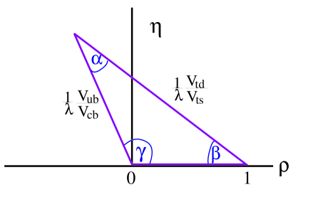
FIGURE 1.: The unitarity triangle shown in the $\rho-\eta$ plane. The left side is determined by measurements of $b\to u/b\to c$ and the right side can be determined using mixing measurements in the $B_{s}$ and $B_{d}$ systems. The angles can be found by making measurements of CP violating asymmetries in hadronic $B$ decays.

The current status of constraints on $\rho$ and $\eta$ is shown in Fig. 2. One constraint on $\rho$ and $\eta$ is given by the $K_{L}^{o}$ CP violation measurement ($\epsilon$)  [?], where the largest error arises from theoretical uncertainty. Other constraints come from current measurements on $V_{ub}/V_{cb}$, and $B_{d}$ mixing  [?]. The widths of both of these bands are dominated by theoretical errors. Note that the errors used are $\pm 1\sigma$. This shows that the data are consistent with the standard model but do not pin down $\rho$ and $\eta$.

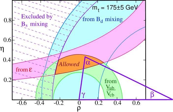
FIGURE 2.: The regions in $\rho-\eta$ space (shaded) consistent with measurements of CP violation in $K_{L}^{o}$ decay ($\epsilon$), $V_{ub}/V_{cb}$ in semileptonic $B$ decay, $B_{d}^{o}$ mixing, and the excluded region from limits on $B_{s}^{o}$ mixing. The allowed region is defined by the overlap of the 3 permitted areas, and is where the apex of the CKM triangle sits. The bands represent $\pm 1\sigma$ errors. The error on the $B_{d}$ mixing band is dominated by the parameter $f_{B}$. Here the range is taken as $240>f_{B}>160$ MeV.

It is crucial to check if measurements of the sides and angles are consistent, i.e., whether or not they actually form a triangle. The standard model is incomplete. It has many parameters including the four CKM numbers, six quark masses, gauge boson masses and coupling constants. Perhaps measurements of the angles and sides of the unitarity triangle will bring us beyond the standard model and show us how these parameters are related, or what is missing.

III The Main Physics Goals of BTeV

A Physics Goals For B’s

Here we briefly list the main physics goals of BTeV for studies of the $b$ quark.

$\bullet$ Precision measurements of $B_{s}$ mixing, both the time evolution, $x_{s}$, and the lifetime difference, $\Delta\Gamma$, between the positive CP and negative CP final states.

$\bullet$ Measurement of the “CP violating” angles $\alpha$ and $\gamma$. We will use $B^{o}\to\pi^{+}\pi^{-}$ for $\alpha$  [?] and measure $\gamma$ using several different methods including measuring the time dependent asymmetry in $B_{s}^{o}\to D_{s}^{\pm}K^{\mp}$, and measuring the decay rates $B^{+}\to D^{o}K^{+}$ and $B^{-}\to\overline{D}^{o}K^{+}$, where the $D^{o}$ can decay directly or via a doubly Cabibbo suppressed decay mode  [?,?].

$\bullet$ Search for rare final states such as $K\mu^{+}\mu^{-}$ and $\pi\mu^{+}\mu^{-}$ which could result from new high mass particles coupling to $b$ quarks.

$\bullet$ We assume that the CP violating angle $\beta$ will have already been measured by using $B^{o}\to\psi K_{s}$, but we will be able to significantly reduce the error.

B The Main Physics Goals for charm

According to the standard model, charm mixing and CP violating effects should be “small.” Thus charm provides an excellent place for non-standard model effects to appear. Specific goals are listed below.

$\bullet$ Search for mixing in $D^{o}$ decay, by looking for both the rate of wrong sign decay, $r_{D}$, and the width difference between positive CP and negative CP eigenstate decays, $\Delta\Gamma$. The current upper limit on $r_{D}$ is $3.7\times 10^{-3}$, while the standard model expectation is $r_{D}<10^{-7}$  [?].

$\bullet$ Search for CP violation in $D^{o}$. Here we have the advantage over $b$ decays that there is a large $D^{*+}$ signal which tags the initial flavor of the $D^{o}$ through the decay $D^{*+}\to\pi^{+}D^{o}$. Similarly $D^{*-}$ decays tag the flavor of initial $\overline{D}^{o}.$ The current experimental upper limits on CP violating asymmetries are on the order of 10%, while the standard model prediction is about 0.1%  [?].

$\bullet$ Search for direct CP violation in charm using $D^{+}$ and $D_{s}^{+}$ decays.

$\bullet$ Search for rare decays of charm, which if found would signal new physics.

C Other $b$ and charm Physics Goals

There are many other physics topics that can be addressed by BTeV. A short list is given here.

$\bullet$ Measurement of the $b\overline{b}$ production cross section and correlations between the $b$ and the $\overline{b}$ in the forward direction.

$\bullet$ Measurement of the $B_{c}$ production cross section and decays.

$\bullet$ The spectroscopy of $b$ baryons.

$\bullet$ Precision measurement of $V_{cb}$ using the usual mesonic decay modes and the baryonic decay mode $\Lambda_{b}\to\Lambda_{c}\ell^{-}\bar{\nu}$ to check the form factor shape predictions.

$\bullet$ Precision measurement of $V_{ub}/V_{cb}$ using the usual mesonic decay modes.

$\bullet$ Measurement of the $c\overline{c}$ production cross section and correlations between the $c$ and the $\overline{c}$ in the forward direction.

$\bullet$ Precision measurement of $V_{cd}$ and the form factors in the decays $D\to\pi\ell^{+}\nu$ and $D\to\rho\ell^{+}\nu$.

$\bullet$ Precision measurement of $V_{cs}$ and the form factors in the decay $D\to K^{*}\ell^{+}\nu$.

IV Characteristics of Hadronic $b$ Production

It is often customary to characterize heavy quark production in hadron collisions with the two variables $p_{t}$ and $\eta$. The latter variable was invented by those who studied high energy cosmic rays and is assigned the value

$$\eta=-ln\left(\tan\left({\theta/2}\right)\right),$$ (3)

where $\theta$ is the angle of the particle with respect to the beam direction.

According to QCD-based calculations of $b$-quark production, the $b$’s are produced “uniformly” in $\eta$ and have a truncated transverse momentum, $p_{t}$, spectrum, characterized by a mean value approximately equal to the $B$ mass  [?]. The distribution in $\eta$ is shown in Fig. 3.

FIGURE 3.: The $B$ yield versus $\eta$ (left). $\beta\gamma$ of the $B$ versus $\eta$ (right). Both plots are for the Tevatron.

There is a strong correlation between the $B$ momentum and $\eta$. Shown also in Fig. 3 is the $\beta\gamma$ of the $B$ hadron versus $\eta$. It can clearly be seen that near $\eta$ of zero, $\beta\gamma\approx 1/2$, while at larger values of $|\eta|$, $\beta\gamma$ can easily reach values of  6. This is important because the observed decay length increases with $\beta\gamma$ and furthermore the absolute momenta of the decay products are larger allowing for a suppression of the multiple scattering error.

The “flat” $\eta$ distribution hides an important correlation of $b\bar{b}$ production at hadron colliders. In Fig. 4 the production angle of the hadron containing a $b$ quark is plotted versus the production angle of the hadron containing a $\bar{b}$ quark according to the Pythia generator. There is a very strong correlation in the forward direction (the direction of the $p$ beam at 0^∘-0^∘), where both $B$ and $\overline{B}$ hadrons are going in the same direction. The same strong correlation is present in the $\overline{p}$ direction. This correlation is not present in the central region (near 90^∘). By instrumenting a relatively small region of angular phase space, a large number of $b\bar{b}$ pairs can be detected. Furthermore the $B$’s populating the two “forward” regions have large values of $\beta\gamma$.

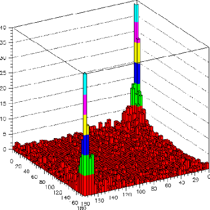
FIGURE 4.: The production angle (in degrees) for the hadron containing a $b$ quark plotted versus the production angle for the hadron containing a $\bar{b}$ quark.

Charm production is similar to $b$ production but more copius. Current theoretical estimates are that charm is 1-2% of the total $p\bar{p}$ cross section.

Table  1 gives the relevant Tevatron parameters. We expect to eventually run at a luminosity of $2\times 10^{32}$cm^-2s^-1. A machine design that holds the luminosity constant at this value, called “luminosity leveling,” has been developed. We plan to adopt this design.

TABLE 1.: The Tevatron as a $b$ and $c$ source for C0 in Run II.

Luminosity	$2\times 10^{32}$ cm-2s-1
$b$ cross section	100 $\mu$b
# of $b$’s per 107 sec	$4\times 10^{11}$
$b$ fraction	0.2%
$c$ cross section	$>500~{}\mu$b
Bunch spacing	132 ns
Luminous region length	$\sigma_{z}$ = 30 cm
Luminous region length	$\sigma_{x}$ $\sigma_{y}$ = $\approx 50$ $\mu$m
Interactions/crossing	$<2>$

V The Experimental Technique: A Forward Two-arm Spectrometer

A sketch of the apparatus is shown in Fig. 5. The two-arm spectrometer fits in the expanded C0 interaction region, which is being excavated. The magnet that we will use, called SM3, exists at Fermilab. The other important parts of the experiment include the vertex detector, the RICH detectors, the EM calorimeters and the muon system.

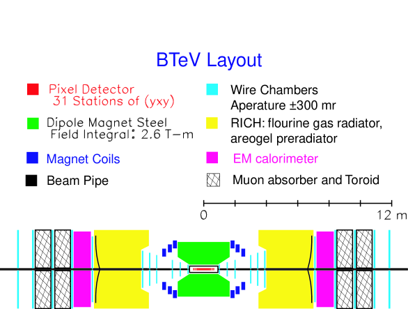
FIGURE 5.: Sketch of the BTeV spectrometer.

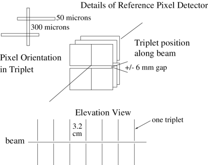
FIGURE 6.: Layout of the BTeV pixel detector. There are 31 stations of triplets with the narrow pixel dimension in the bend plane. The most recent version replaces the 12 mm gap between detector planes with a 12 mm $\times$ 12 mm square hole centered on the beam.

The angle subtended is approximately $\pm$300 mr in both plan and elevation views. The vertex detector is a multi-plane pixel device that sits inside the beam pipe. The baseline design has 31 stations with triplets in each station. The detector is sketched in Fig. 6. Our new baseline detector has a square hole, 12 mm $\times$ 12 mm around the beam, instead of a 12 mm gap between top and bottom halves. (Some of our simulations have been done with the detector with the gap, called “EOI,” and some have been done with the “square hole.”) The triggering concept is to pipeline the data and to detect detached $b$ or $c$ vertices in the first trigger level. The vertex detector is put in the magnetic field in order to insure that the tracks considered for vertex based triggers do not have large multiple scattering because they are low momentum.

The RICH detector [?] has a gas radiator, either C₄F₁₀ or C₅F₁₂, and mirrors that focus the Cherenkov light onto photodectors situated outside of the fiducial volume of the detector. This system will provide $K/\pi$ separation in the momentum range between 3 and 70 GeV/c. To resolve protons from kaons below the kaon threshold of 9 GeV/c, a thin aerogel radiator may be placed in front of the gas volume. The same photon detector would be utilized.

The muon detector consists of position-measuring chambers placed around and between an iron slab followed by another slab used as a magnetized toroid. This system is used both to trigger on final states with dimuons and to identify muons in the final analysis.

VI Simulations

A Introduction

We have developed several fast simulation packages to verify the basic BTeV concepts and aid in the final design. The trigger simulations, discussed below, are done with full pattern recognition. The input consists only of hits which are smeared by their resolution. To simulate backgrounds in the final physics analysis, we use a fast simulation which simulates track resolutions but not the pattern recognition. This is done because we have to simulate backgrounds in processes with branching ratios in the 10^-5-10^-6 range and we cannot afford the computer time. The key program in our system is MCFast  [?]. Charged tracks are generated and traced through different material volumes including detector resolution, multiple scattering and efficiency. This allows us to measure acceptances and resolutions in a fast reliable manner.

B Trigger Simulations

We simulate the trigger using the baseline pixel detector shown in Fig. 6. The triplet stations each provide a three-dimensional space point as well as a track direction mini-vector. This is useful for fast pattern recognition. The trigger simulations are carried out by doing the complete pattern recognition from the hits left in the detector by tracks and converted photons.

Our baseline trigger algorithm works by first determining the main event vertex and then finding how many tracks miss this vertex by $n\sigma$, where $\sigma$ refers to the impact parameter divided by its error. Furthermore, a requirement is then placed on the track momentum in the bend plane, $p_{y}$, as determined on line. The preliminary results of simulating this algorithm are shown in Fig. 7 (right) for a cut $p_{y}~{}>~{}0.5$ GeV/c  [?]. The choice of the number of tracks and the impact parameter requirement must eventually be optimized, but what is shown here is the efficiency for accepting light quark events ($u$, $d$, and $s$) for various choices on the number of tracks (curves) and the size of their required impact parameter divided by the error in impact parameter. The efficiency for accepting $B^{o}\to\pi^{+}\pi^{-}$ is shown in the left side. Here the efficiency is given after requiring that both tracks are in the spectrometer and accepted for further analysis. For a “typical” $n\sigma$ cut of 3 and track requirement of 2, the $\pi^{+}\pi^{-}$ trigger efficiency is about 45%, while the light quark background has an efficiency of about 0.8%. Note, that we do not consider $c$ to be a background in this experiment. For a “typical” charm reaction the same trigger gives substantially less than 1% efficiency on charm, while the efficiency for two-body charm decays is approximately 1%.

FIGURE 7.: (left) Trigger efficiency for $B^{o}\to\pi^{+}\pi^{-}$ for pion tracks in the spectrometer. (right) Trigger efficiency for light quark events. The ordinate gives the choice of cut value on the impact parameter in terms of number of standard deviations ($\sigma$) of the track from the primary vertex. The curves show the effect of requiring different numbers of tracks.

The trigger efficiency on states of interest is correlated with the analysis criteria used to reject background. These criteria generally are focussed upon insuring that the $B$ decay track candidates come from a detached vertex, that the momentum vector from the $B$ point back to the primary interaction vertex, and that there are no other tracks consistent with the $B$ vertex. When the analysis criteria are applied first and the trigger efficiency evaluated after, the trigger efficiency defined in this manner is larger. In Fig. 8 we show the efficiency to trigger on $B_{s}\to\psi K^{*o}$, $\psi\to\mu^{+}\mu^{-}$, $K^{*o}\to K^{-}\pi^{+}$ using the tracking trigger only for events with the four tracks in the geometric acceptance, and the efficiency evaluated after all the analysis cuts have been applied. Here the trigger efficiencies for $3\sigma$ and 2 tracks are 67% for events with all 4 tracks in the geometrical acceptance and 84% on events after all the analysis cuts have been applied.

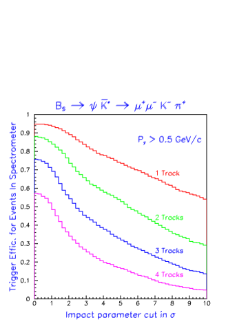
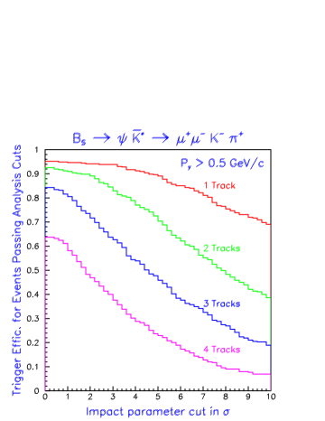
FIGURE 8.: Trigger efficiency of $B_{s}\to\psi K^{*o}$, $\psi\to\mu^{+}\mu^{-}$, $K^{*o}\to K^{-}\pi^{+}$ for tracks in the geometric Acceptance (left) and after all analysis cuts (right). The abscissa gives the value of the impact parameter in terms of number of standard deviations ($\sigma$) of the track from the primary vertex. The curves show the effect of requiring different numbers of tracks. All tracks are required to have at least 0.5 GeV/c momentum in the bend plane.

At the BTeV design luminosity of 2$\times$10³²cm^-2s^-1 there is an average of two interactions per beam crossing. The interactions are spread out over the long ($\sigma$=30 cm) interaction region. The trigger must not fire merely due to the presence of two nearby interactions. To insure this we have imposed a requirement that the maximum impact parameter of a track not be larger than 2 mm. The yield for events containing a $B^{o}\to\pi^{+}\pi^{-}$ decay as a function of luminosity is shown in Fig. 9 (left). Here we do not want the trigger rate to increase as a function of luminosity, even though this means that the efficiency on this rare final state increases. Therefore, a linear rise would be ideal. On the right side we show the probability to trigger on light quark background. We would like this to remain constant with increasing luminosity. No increase occurs up to a luminosity of 10³²cm^-2s^-1, after which the probability for this particular trigger condition increases mildly. However, the first level trigger rate is clearly much lower than the 1% we require until we exceed a luminosity of $\approx 3\times$10³²cm^-2s^-1.

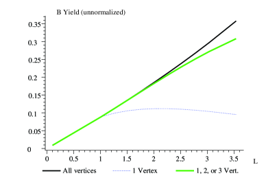
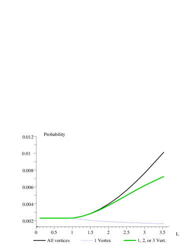
FIGURE 9.: Luminosity dependent trigger efficiencies for $B^{o}\to\pi^{+}\pi^{-}$ (left), and light quark events (right). The abscissa is in units of 10³²cm^-2s^-1.

C Measurement of the CP violating asymmetry in $B^{o}\to\pi^{+}\pi^{-}$

The trigger efficiency for this mode has already been discussed. For the $B^{o}\to\pi^{+}\pi^{-}$ channel BTeV has compared the offline fully reconstructed decay length distributions in the forward geometry with that of a detector configured to work in the central region. The left side plot in Fig. 10 shows the $B$ momentum distribution and decay distance error as a function of $b$ momentum.

The right plot in Fig. 10 shows the normalized decay length expressed in terms of $L/\sigma$ where $L$ is the decay length and $\sigma$ is the error on $L$ for the $B^{o}\to\pi^{+}\pi^{-}$ decay  [?].

The forward detector clearly has a much more favorable $L/\sigma$ distribution, which is due to the excellent proper time resolution. The ability to keep high efficiency in the trigger and analysis levels and devastate the backgrounds relies primarily on having the excellent $L/\sigma$ distribution shown for the forward detector.

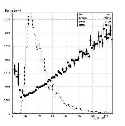
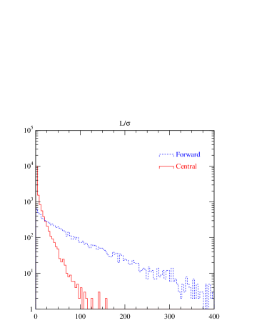
FIGURE 10.: (left) The $B$ momentum distribution for events in the detector acceptance (dashed line) and the error on the spatial distance of the $\pi^{+}\pi^{-}$ decay vertex from the primary vertex (solid points). (right) Comparison of the $L/\sigma$ distributions for the decay $B^{o}\to\pi^{+}\pi^{-}$ in central and forward detectors produced at a hadron collider with a center of mass energy of 1.8 TeV.

For this analysis $L/\sigma$ is required to be $>15$. Each pion track is required to miss the primary vertex by a distance/error $>5\sigma$ and the $B^{o}$ candidate is required to point back to the primary with a distance/error $<2\sigma$. Furthermore, each track must be identified as a pion and not a kaon in the RICH detector. Without particle identification it is impossible to distinguish $B^{o}\to\pi^{+}\pi^{-}$ from the combination of $B^{o}\to K^{\pm}\pi^{\mp}$, $B_{s}\to K^{+}K^{-}$ and $B_{s}\to K^{\pm}\pi^{\mp}$, as is shown on Fig. 11. Here $\cal{B}$$(B^{o}\to K^{\pm}\pi^{\mp})$ is taken as $1.5\times 10^{-5}$ and $\cal{B}$$(B^{o}\to\pi^{+}\pi^{-})$ is taken as $0.75\times 10^{-5}$, from recent CLEO measurements  [?]. The $B_{s}$ decay into $K^{+}K^{-}$ is assumed to have the same rate as the $B^{o}$ decay into $K^{\pm}\pi^{\mp}$, and the $B_{s}$ decay into $K^{\pm}\pi^{\mp}$ is assumed to have the same rate as the $B^{o}$ decay into $\pi^{+}\pi^{-}$.

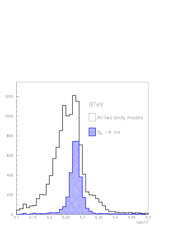
FIGURE 11.: Invariant mass distributions of all $B\to h^{+}h^{-}$ final states, where $h$ denotes either a pion or kaon, and the mass is computed assuming that both tracks are pions. The plot on the left shows the individual background channels and the one on the right shows the sum of all channels properly normalized (see text) to the $\pi^{+}\pi^{-}$ signal.

Using the good particle identification, BTeV predicts that they can measure the CP violating asymmetry in $\pi^{+}\pi^{-}$ to $\pm 0.013$ as detailed in Table 2.

TABLE 2.: Numbers entering into the accuracy in measuring the CP violating asymmetry in $B^{o}\to\pi^{+}\pi^{-}$.

Quantity	Value
Cross section	100 $\mu$b
Luminosity	$2\times 10^{32}$
# of $B^{o}$/2$\times 10^{7}$s, $\cal{L}$ leveled	$2.8\times 10^{11}$
$\cal{B}$$(B^{o}\to\pi^{+}\pi^{-})$	$0.75\times 10^{-5}$
Reconstruction efficiency	0.08
Triggering efficiency (after all other cuts)	0.72
# of $\pi^{+}\pi^{-}$	128,000
$\epsilon D^{2}$ for flavor tags ($K^{\pm}$, $\ell^{\pm}$, same + opposite sign jet tags)	0.1
# of tagged $\pi^{+}\pi^{-}$	12,800
Signal/Background	0.9
Error in asymmetry (including background)	$\pm 0.013$

D Flavor tagging

We have assumed a flavor tagging efficiency of 10%. Actually our studies show that we probably can achieve a higher efficiency. The usual definitions are: $N$ is the number of reconstructed signal events, $N_{R}$ is the number of right sign flavor tags, $N_{W}$ is the number of wrong sign flavor tags, $\epsilon$ is the efficiency (given by $[N_{R}+N_{W}]/N$) and $D$ is the dilution (given by $[N_{R}-N_{W}]/[N_{R}+N_{W}]$). The quantity of interest is $\epsilon D^{2}$ which when multiplied by $N$ gives the effective number of events useful for the calculation of an asymmetry error.

We have investigated the feasibility of tagging kaons using a gas Ring Imaging Cherenkov Counter (RICH) in a forward geometry and compared it with what is possible in a central geometry using Time-of-Flight counters with good, 100 ps, resolution. For the forward detector the momentum coverage required is between 3 and 70 GeV/c. The lower momentum value is determined by our desire to tag charged kaons for mixing and CP violation measurements, while the upper limit comes from distinguishing the final states $\pi^{+}\pi^{-}$, $K^{+}\pi^{-}$ and $K^{+}K^{-}$. The momentum range is much lower in the central detector but does have a long tail out to about 5 GeV/c. Either C₄F₁₀ or C₅F₁₂ have pion thresholds of about 2.5 GeV/c. The kaon and proton thresholds for the first gas are 9 and 17 GeV/c, respectively.

The BTeV RICH was simulated using the current C0 geometry with MCFast. Fig. 12 shows the number of identified kaons plotted versus their impact parameter divided by the error in the impact parameter for both right-sign and wrong-sign kaons. A right-sign kaon is a kaon that properly tags the flavor of the other $B$ at production. We expect some wrong-sign kaons from mixing and charm decays. Many others just come from the primary. A cut on the impact-parameter standard-deviation plot at $3.5\sigma$ gives an overall $\epsilon D^{2}$ of 6%. This number is reduced to 5% because of $b\overline{b}$ mixing  [?]. Without the aerogel preradiator to distinguish protons from kaons below threshold we would experience an additional reduction down to about 4%. These numbers are for a perfect RICH system. Putting in a fake rate of several percent, however, does not significantly change the conclusion.

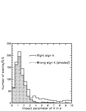
FIGURE 12.: (left) $L/\sigma$ distributions in BTeV for $K^{\pm}$ impact parameters for right sign (unshaded) and wrong sign (shaded) tags. (right) Overall $\epsilon$D² values from kaon tagging for a forward detector containing a flourine based RICH versus a central detector with 100 ps time of flight resolution as a function of kaon impact parameter in units of $L/\sigma$. (Protons and $b\overline{b}$ mixing have been ignored in both cases.)

The simulation of the central detector gives much poorer numbers. In Fig. 12 $\epsilon D^{2}$ for both the forward and central detectors are shown as a function of the kaon impact parameter (protons have been ignored). It is difficult to get $\epsilon D^{2}$ of more than 1.5% in the central detector.

Now let us consider other tags. We have simulated muon and electron flavor tags in our system. Although this technique is very useful at $e^{+}e^{-}$ colliders operating at the $\Upsilon(4S)$, it is less useful here because it is difficult to distinguish leptons from the $b\to c\to\ell^{+}$ decay from the primary leptons from the $b$ quark decay. Our estimates are given in Table 3 along with those for a central detector.

TABLE 3.: The projected flavor tagging efficiencies for a central detector similar to CDF and BTeV in units of $\epsilon D^{2}$.

	$K^{\pm}$	$\mu^{\pm}$	$e^{\pm}$	SST	Jet Charge	Sum
BTeV	5%	1.6%	1.0%	$>$2%	6.5%	$>$10%
Central	0%	1.0%	0.7%	2%	3%	$\approx$5%

The two other methods considered are “jet charge” and “same side” tagging (sst). We have not yet studied sst, which is using the charge of a track closest in phase space to the reconstructed $B$. However, CDF has measured $\epsilon D^{2}$ for it to be (1.5$\pm$0.4)% and take 2% as their future projection using an improved vertex detector. We have studied jet charge, which involves taking a weighted measure of the charge of the tagging $b$ jet. However, we incorporate information on the detachment of the tracks to help us define the jet. CDF extrapolates to 3% while we expect 6.5%. Table 3 summarizes our projected tagging efficiencies.

E Measurement of $B_{s}$ mixing

BTeV has studied the feasibility of measuring the $B_{s}$ mixing parameter $x_{s}$ = $\Delta m_{s}/\Gamma_{s}$. This measurement is key to obtaining the right side of the unitarity triangle shown in Fig. 1. Current limits on $B_{s}$ mixing from LEP give $x_{s}>15$  [?]. Recall that for $B_{d}$ mesons, $x$ = 0.73. The oscillation length for $B_{s}$ mixing is at least a factor of 20 shorter and may approach a factor of 100!

BTeV has investigated two final states that can be used. The first, $\psi K^{*o}$, $\psi\to\mu^{+}\mu^{-}$ and $K^{*o}\to K^{-}\pi^{+}$, has several advantages. It can be selected using either a dilepton or detached vertex trigger. Backgrounds can be reduced in the analysis by requiring consistency with the $\psi$ and $K^{*o}$ masses. Furthermore, it should have excellent time resolution as there are four tracks coming directly from the $B$ decay vertex. The resolution in proper time is 42 fs. The one disadvantage is that the decay is Cabibbo suppressed, the Cabibbo allowed channel being $\psi\phi$ which is useless for mixing studies. The branching ratio therefore is predicted to have the low value of $8.5\times 10^{-5}$.

The time distributions of the unmixed and mixed decays are shown in Fig. 13, along with a calculation of the likelihood of there being an oscillation as determined by fits to the time distributions. Background and wrong tags are included.

FIGURE 13.: The observed decay time distributions for $B_{s}\to\psi K^{*o}$ generated with $x_{s}=40$. Unmixed decays are shown in (a), mixed in (b). Background and mistagging have been included. In (c) the results of a likelihood fit to the time distributions are shown. The dashed line shows a 5$\sigma$ difference from the best solution.

The fitting procedure correctly finds the input value of $x_{s}=40$. The danger is that a wrong solution will be found. The dashed line shows the change in likelihood corresponding to 5 standard deviations. If our criterion is that the next best solution be greater than $5\sigma$, then this is the best that can be done with one year’s worth of data in this mode. Once a clean solution is found, the error on $x_{s}$ is quite small, being $\pm 0.15$ in this case.

BTeV has also investigated the $D_{s}^{+}\pi^{-}$ decay of the $\overline{B}_{s}$, with $D_{s}^{+}\to\phi\pi^{+}$. It turns out that the lifetime resolution is 45 fs, almost the same as for the $\psi K^{*o}$ decay mode. Since the predicted branching ratio for this mode is 0.3%, we obtain 19200 events in one year of running, with a signal to background of 3:1. Fig. 14 shows the $x_{s}$ reach obtainable for a $5\sigma$ discrimination between the favorite solution and the next best solution, for both decay modes. The background is assumed to be 20% and the flavor mistag fraction is taken as 25%. The tagging efficiency is taken as 10%. The absicca gives the number of years of running, where one year is $10^{7}$ seconds. The pixel system with the 12 mm gap is called the EOI detector here.

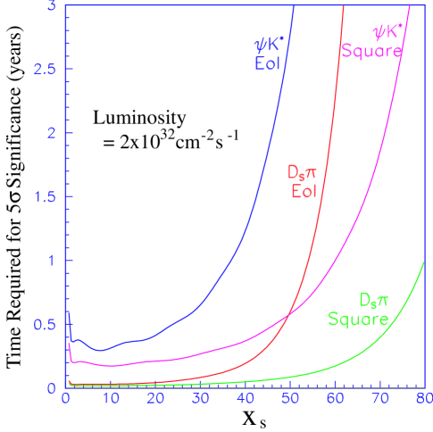
FIGURE 14.: The $x_{s}$ reach for both $D_{s}^{+}\pi^{-}$ and $\psi K^{*o}$ decays of the $\overline{B}_{s}$. The EOI detector has a 12 mm gap between upper and lower halves of the pixel detector, while the square hole has a 12x12 mm² hole. The calculation is for non-leveled luminosity.

The other detector configuration that we simulated has the pixels configured around the beam leaving a 12 mm $\times$ 12 mm square hole. This detector has better efficiency and time resolution (see section V) and now has become the BTeV baseline.

The $x_{s}$ reach is excellent and extends over the entire predicted Standard Model range.

F Measurement of $\gamma$

The angle $\gamma$ could in principle be measured using a CP eigenstate of $B_{s}$ decay that was dominated by the $b\to u$ transition. One such decay that has been suggested is $B_{s}\to\rho^{o}K_{s}$. However, there are the same “Penguin pollution” problems as in $B^{o}\to\pi^{+}\pi^{-}$, but they are more difficult to resolve in the vector-pseudoscalar final state. (Note, the pseudoscalar-pseudoscalar final state here is $\pi^{o}K_{s}$, which does not have a measurable decay vertex.)

Fortunately, there are other ways of measuring $\gamma$. CP eigenstates are not used, which introduces discrete ambiguities. However, combining several methods should remove these.

We have studied three methods of measuring $\gamma$. The first method uses the decays $B_{s}\rightarrow D_{s}^{\pm}K^{\mp}$ where a time-dependent CP violation can result from the interference between the direct decay and the mixing induced decay  [?]. Fig. 15 shows the two direct decay processes for $\overline{B}^{o}_{s}$.

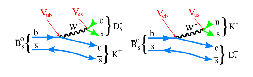
FIGURE 15.: Two diagrams for $\overline{B}_{s}^{o}\to D_{s}^{\pm}K^{\mp}$.

Consider the following time-dependent rates for neutral $B$ mesons to non-CP eigenstates via two different processes that can be separately measured using flavor tagging of the other $b$:

$${\Gamma}(B_{s}\rightarrow f)=|M|^{2}e^{-{t}}\{\cos^{2}(xt/2)+\rho^{2}\sin^{2}(xt/2)-\rho{\sin(\phi+\delta)}\sin(xt)\}$$

$$\Gamma(\bar{B_{s}}\rightarrow\bar{f})=|M|^{2}e^{-{t}}\{\cos^{2}(xt/2)+\rho^{2}\sin^{2}(xt/2)+\rho{\sin(\phi-\delta)}\sin(xt)\}$$

$$\Gamma(B_{s}\rightarrow\bar{f})=|M|^{2}e^{-{t}}\{\rho^{2}\cos^{2}(xt/2)+\sin^{2}(xt/2)-\rho{\sin(\phi-\delta)}\sin(xt)\}$$

$$\Gamma(\bar{B_{s}}\rightarrow f)=|M|^{2}e^{-{t}}\{\rho^{2}\cos^{2}(xt/2)+\sin^{2}(xt/2)+\rho{\sin(\phi+\delta)}\sin(xt)\},$$

where $M=\langle~{}f|B\rangle$, $\rho=\frac{\langle~{}f|\bar{B}\rangle}{\langle~{}f|{B}\rangle}$, $\phi$ is the weak phase between the two amplitudes and $\delta$ is the strong phase between the two amplitudes. The three parameters $\rho$, $\sin(\phi+\delta),\sin(\phi-\delta)$ can be extracted from a time-dependent study if $\rho=O(1)$.

In the case of $B_{s}$ decays where $f=D_{s}^{+}K^{-}$ and $\bar{f}=D_{s}^{-}K^{+}$, the weak phase is $\gamma$. The decay modes $B_{s}\rightarrow D_{s}^{+}K$, $D_{s}^{+}\rightarrow\phi\pi^{+}$, $\phi\rightarrow K^{+}K^{-}$, or $D_{s}\rightarrow K^{*o}K^{+}$, were simulated. For the $\phi\pi^{+}$ mode, the combined geometric acceptance and reconstruction efficiency is 5.2% with S/B=10  [?], and the trigger efficiency is 67%. In the $K^{*o}K^{+}$ mode the geometric and reconstruction efficiency is 5.9% and the trigger efficiencies and signal to background are same as in the $\phi\pi^{+}$ mode. Using the branching fractions predicted by Aleksan  [?] and assuming a tagging efficiency $\epsilon=15\%$ we expect 8900 events in 2$\times 10^{7}$ s.

The decay time resolution and the detachment of the decay vertex from the primary production vertex are shown in Fig. 16 for the $D_{s}^{+}\to\phi\pi^{+}$ decay mode. The distributions for the $K^{*o}K^{+}$ mode are similar.

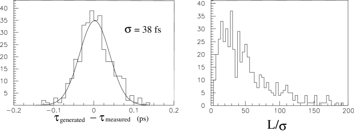
FIGURE 16.: (left) The generated minus measured proper time distribution for $\overline{B}_{s}^{o}\to D_{s}^{\pm}K^{\mp}$, $D_{s}^{+}\to\phi\pi^{+}$. (right) The distribution in $L/\sigma$ for this mode.

Using the measured values of S/B and time resolution, a mistag rate of 25%, and $x_{s}$=20, a mini-Monte Carlo was used to generate the extracted value of $\gamma$ for an ensemble of experiments each with 8900 signal events, for various sets of input parameters $\rho$, $\sin(\gamma+\delta),\sin(\gamma-\delta)$. A maximum likelihood fit was then used to extract fitted values of the parameters.

Fig. 17 shows the distributions of the parameters with input values $\rho$=0.5, $\sin\gamma=0.866$ and $\cos\delta=0.7$. Assuming that $\sin\gamma>0$ then $\sin\gamma$ can be determined up to a two-fold ambiguity, hence $\gamma$ up to a four-fold ambiguity.

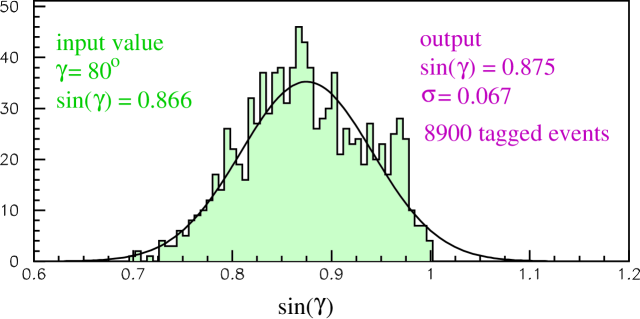
FIGURE 17.: Results of determining $\gamma$ for many different “experiments” with input value of $\gamma$=80^∘ using the decay time distributions for $\overline{B}_{s}^{o}\to D_{s}^{\pm}K^{\mp}$.

Another method for extracting $\gamma$ has been proposed by Atwood, Dunietz and Soni  [?], who refined a suggestion by Gronau and Wyler  [?]. A large CP asymmetry can result from the interference of the decays $B^{-}\rightarrow K^{-}D^{0},D^{0}\rightarrow f$ and $B^{-}\rightarrow K^{-}\overline{D}^{0},\overline{D}^{0}\rightarrow f$, where $f$ is a doubly Cabibbo suppressed decay of the $D^{0}$ (for example $f=K^{+}\pi^{-},K\pi\pi$, etc.) Since $B^{-}\rightarrow K^{-}\overline{D}^{0}$ is color-suppressed and $B^{-}\rightarrow K^{-}D^{0}$ is color-allowed, the overall amplitudes for the two decays are expected to be approximately equal in magnitude. The weak phase difference between them is $\gamma$. To observe a CP asymmetry there must also be a non-zero strong phase between the two amplitudes. It is necessary to measure the branching ratio ${\cal B}(B^{-}\rightarrow K^{-}f)$ for at least 2 different states $f$ in order to determine $\gamma$ up to discrete ambiguities. We have examined the decay modes $B^{-}\rightarrow K^{-}[K^{+}\pi^{-}]$ and $B^{-}\rightarrow K^{-}[K^{+}3\pi]$. The combined geometric acceptance and reconstruction efficiency was found to be 6.6% for the $K\pi$ mode and 5.5% for $K3\pi$ with a signal to background of about 1:1. The trigger efficiency is approximately 70% for both modes. The expected number of $B^{\pm}$ events in $10^{7}$ s is 2400 in the $K\pi$ mode and 4200 in the $K3\pi$ mode. With this number of events we expect to be able to measure $\gamma$ (up to discrete ambiguities) with a statistical error of about ${\pm}8^{\circ}$ in one year of running at ${\cal L}=2\times 10^{32}{\rm cm}^{-2}{\rm s}^{-1}$. The overall sensitivity depends on the actual values of $\gamma$ and the strong phases.

The next method, described by Gronau and Rosner  [?] and Fleischer and Mannel  [?], uses $B^{0}\rightarrow K^{+}\pi^{-}$ and $B^{+}\rightarrow K^{0}\pi^{+}$ decays. It is particularly promising as it may complement other methods by excluding some of the region around $\gamma=\pi/2$. We expect to reconstruct 3600 $B^{\pm}\rightarrow K_{s}\pi^{\pm}$ with S/B=0.5 and 29000 $B^{0}/\overline{B}^{0}\rightarrow K^{\pm}\pi^{\mp}$ with S/B=3. Gronau and Rosner estimate a measurement of $\gamma$ to $10^{\circ}$ with 2400 events in each channel  [?], however there has been much theoretical discussion about the effects of isospin conservation and rescattering which casts doubt on this method  [?] [?] [?] [?]. There have been several suggestions, however, on how to measure these effects  [?], and this method may turn out to be useful.

VII Decay Time Resolution

In all of these studies we have assumed that we would have 9 $\mu$m spatial resolution in each track hit in the pixel plane. We now address the question of whether or not this is reasonable.

The parameters affecting the pixel resolution include the size of the pixel, the use of binary (one bit) versus analog (4 bits) information, threshold and gain variations, and the use of electrons or holes as charge carriers, since the drift velocity for electrons is three times that for holes. For different incident angles of tracks on the pixels the charge sharing is affected by the magnetic field. In BTeV we use a 1.5 T dipole field.

In Fig. 18(a) we show the track angle distribution for two $B$ final states, the two-body state $\pi^{+}\pi^{-}$ and the four-body state $\pi^{+}K^{+}K^{-}K^{-}$. In both cases the angular distribution peaks at small angles, about 50 mr and then falls slowly towards larger angles. The spatial resolution has been simulated as a function of angle for various pixel sizes. The baseline size is 50 $\mu$m $\times$ 300 $\mu$m. The results of the simulation for this size are shown in Fig. 18(b). The magnetic field is in the y direction in this case. So the tracks hitting the x layers are bent. The resolution using binary readout is about 10 $\mu$m, while it is about 5 $\mu$m using 4-bit analog. Note that the poorer resolution peak near zero degrees in the non-bend plane does exist in the bend plane, but it is shifted toward negative incident angles. Similar results are obtained with holes as charge carriers.

FIGURE 18.: (left) The distribution of track angles with respect to the pixel planes for tracks with at least 9 hits for $B^{o}\to\pi^{+}\pi^{-}$ and $B^{o}\to\pi^{+}K^{-}K^{+}K^{-}$ decays. (right) The spatial resolution for the X (bend plane) and Y directions, separately, as a function of projected angle, $\Theta_{x,(y)}$, for binary and 4-bit analog readout using a pixel size of 50$\times$300 $\mu$m².

The resolution in proper time is affected by several factors. One is the inherent pixel resolution, as discussed above. Others include the amount of material in the pixel system, and the distance the pixel detector is placed from the beam line. We take the latter as 6 mm. This distance is limited by the maximum amount of radiation damage we are willing to sustain. (The system is retractable during machine injection.) In Fig. 19 we show the proper time resolution achievable on the $\psi K^{*o}$ decay of the $B_{s}$ for several different detector geometries as a function of the spatial resolution. The circles represent a geometry with a 12 mm gap and equivalent silicon thickness of 600, 500, and 600 $\mu$m for the three layers. These include the 300 $\mu$m of silicon for each layer, a radio-frequency shield of 100 $\mu$m of Al and material for electronics and cooling.

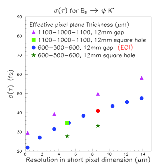
FIGURE 19.: The calculated proper time resolutions for the decay mode $B_{s}\to\psi K^{*o}$, $K^{*o}\to K^{-}\pi^{+}$ as a function of spatial resolution in the pixel system for different detector geometries and thicknesses. The two geometries considered are a gap of 12 mm between two halves of the pixel system and square hole of 12mm $\times$ 12 mm. The equivalent silicon thicknesses for the three planes are listed.

The simulations presented here have assumed a 9 $\mu$m spatial resolution, even though we believe that 5 $\mu$m is possible. The equivalent silicon thickness of a three plane station is taken at 1700 $\mu$m. A detector of twice the material thickness and 5 $\mu$m resolution would have the same time resolution as the one we have been using. This points out the need to minimize the material, a well known lesson.

VIII Comparisons with other experiments

A Comparisons with $e^{+}e^{-}$ $B$-factories

Most of what is known about $b$ decays has been learned at $e^{+}e^{-}$ machines  [?]. Machines operating at the $\Upsilon(4S)$ found the first fully reconstructed $B$ mesons (CLEO), $B^{o}$-$\overline{B}^{o}$ mixing (ARGUS), the first signal for the $b\to u$ transition (CLEO), and Penguin decays (CLEO). Lifetimes of $b$ hadrons were first measured by experiments at PEP, slightly later at PETRA, and extended and improved by LEP  [?].

The success of the $\Upsilon(4S)$ machines has led to the construction at KEK and SLAC of two new $\Upsilon(4S)$ machines with luminosity goals in excess of $3\times 10^{33}$cm^-2s^-1. These machines will have asymmetric beam energies so they can measure time dependent CP violation. They will join an upgraded CESR machine at Cornell with symmetric beam energies. These machines will investigate only $B^{o}$ and $B^{\pm}$ decays, they will not investigate $B_{s}$, $B_{c}$ or $\Lambda_{b}$ decays.

Table 4 shows a comparison between BTeV and an asymmetric $e^{+}e^{-}$ machine for measuring the CP violating asymmetry in the decay mode $B^{o}\to\pi^{+}\pi^{-}$. It is clear that the large hadronic $b$ production cross section can overwhelm the much smaller $e^{+}e^{-}$ rate.

TABLE 4.: Number of tagged $B^{o}\to\pi^{+}\pi^{-}$ ($\cal{B}$=$0.75\times 10^{-5}$)

	$\cal{L}$(cm-2s${}^{-1})$	$\sigma$	# $B^{o}/10^{7}$s	efficiency	$\epsilon D^{2}$	# tagged
$e^{+}e^{-}$	$3\times 10^{33}$	1 nb	$3.0\times 10^{7}$	0.4	0.4	46
BTeV†	$2\times 10^{32}$	100$\mu$b	$1.1\times 10^{11}$	0.06	0.1	6400
BTeV‡	$2\times 10^{32}$	100$\mu$b	$2.1\times 10^{11}$	0.06	0.1	12800
†This is for gap detector, expect increase with square hole
‡Luminosity leveled, use $2\times 10^{7}$ s/year (gap detector)

B Comparisons with Tevatron Central Detectors

Both CDF and D0 have measured the $b$ production cross section  [?] and CDF has contributed to our knowledge of $b$ decay mostly by its measurements of the lifetime of $b$-flavored hadrons  [?], which are competitive with those of LEP  [?] and recently through its discovery of the $B_{c}$ meson  [?]. These detectors were designed for physics discoveries at large transverse momentum. It is remarkable that they have been able to accomplish so much in $b$ physics.

However, these detectors are very far from optimal for $b$ physics. BTeV has been designed with $b$ physics as its primary goal. To have an efficient trigger based on separation of $b$ decays from the primary, BTeV uses the large $\eta$ region where the $b$’s are boosted. The detached vertex trigger allows collection of interesting purely hadronic final states such as $\pi^{+}\pi^{-}$, $D_{s}^{+}\pi^{-}$ and $D_{s}^{+}K^{-}$. It also allows us to collect enough charm to investigate mixing and CP violation.

The use of the forward geometry also allows excellent charged hadron identification with a gaseous RICH detector. This is crucial for many physics issues such as separating $K\pi$ from $\pi\pi$, $D_{s}\pi$ from $D_{s}K$, kaon flavor tagging etc…

C Comparison with LHC-B

LHC-B is an experiment proposed for the LHC with almost the same physics goals as BTeV  [?]. LHC-B has two advantages: the $b$ cross section is five times higher than at the Tevatron while the total cross section is only 1.6 times as large, and the mean number of interactions per crossing is three times lower, because the LHC has bunches every 25 ns, while the Tevatron bunches come every 132 ns.

There are, however, many advantages which accrue to BTeV. Let us first consider the machine specific ones. The 132 ns bunch spacing at the Tevatron makes first level detached vertex triggering easier. It is difficult for the vertex detector electronics in LHC-B to settle in 25 ns. The seven times larger energy at the LHC results in a larger track multiplicity per collision which causes trigger and tracking problems and a larger range of track momenta that need to be analyzed. The interaction region at the LHC is relatively short, $\sigma$=5 cm, compared with the 30 cm long region at Fermilab. This somewhat compensates for the larger number of interactions per crossing, since the interactions are well separated.

There are detector specific advantages for BTeV as well. BTeV is a two-arm spectrometer, resulting a factor of two advantage. BTeV has the vertex detector in the magnetic field which allows the rejection of high multiple scattering (low momentum) tracks in the trigger. Furthermore, BTeV is designed around a pixel vertex detector while LHC-B has a silicon strip detector. BTeV can put the detector closer to the beam (6 mm versus 1 cm), and has a much more robust tracking system which can trigger on detached verticies in the first trigger level, while LHC-B triggers on tracks of moderate transverse momentum in their first trigger level.

We feel that we have more than compensated for LHC-B’s initial advantages.

IX Conclusions

Hadron colliders have large $b$ and $c$ cross sections allowing the opportunity for precision measurements of CP violation and $B_{s}$ mixing. In our view this requires high density tracking and triggering information that can be provided by a state of the art pixel system. BTeV has been designed to fit in the new C0 interaction region at the Tevatron and incorporates a pixel vertex detector, downstream tracking, charged paricle identification, lepton identification and photon detection. The vertex detector enables Level I vertex triggering and excellent time resolution on heavy hadron decays  [?].

A summary of the physics reach is shown in Table 5. Those simulations that have been upgraded by using the square hole detector are so indicated.

TABLE 5.: BTeV Physics Reach

Measurement	Accuracy in $10^{7}$ s
	${\cal L}=2\times 10^{32}$, $\cal{L}$ leveled
$x_{s}$ (square hole)	up to 80 & beyond
$A_{CP}(B^{0}\rightarrow\pi^{+}\pi^{-})$ (gap)	$\pm 0.013$
$\gamma$ using $D_{s}K^{-}$ (square hole)	$\pm 8^{\circ{\dagger}}$
$\gamma$ using $D^{0}K^{-}$ (square hole)	$\pm 8^{\circ{\ddagger}}$
${\cal B}(B^{-}\rightarrow K^{-}\mu^{+}\mu^{-})$ (gap)	$4\sigma$ at ${\cal B}$ of $5.4\times 10^{-8}$
$\sin(2\beta)$ using $B^{o}\to\psi K_{s}$ (square hole)	$\pm 0.013$
†Assumes $\rho$=0.7, $\cos\delta$=0.7, $\sin\gamma$=0.5, $x_{s}$=20
‡For most values of strong phases and $\gamma$

BTeV is an officially recognized R&D project at Fermilab. Development has started on the pixel, trigger, RICH, muon, forward tracking and electromagnetic calorimeter systems. More information on BTeV can be found on the world-wide-web  [?].

REFERENCES

- 1. The CESR B Physics Working Group, K. Lingel et al, “Physics Rationale For a B Factory”, Cornell Preprint CLNS 91-1043 (1991); SLAC Preprint SLAC-372 (1991); “Progress Report on Physics and Detector at KEK Asymmetric B Factory,” KEK Report 92-3 (1992)
- 2. N. Cabibbo, Phys. Rev. Lett. 10, 531 (1963); M. Kobayashi and K. Maskawa, Prog. Theor. Phys. 49, 652 (1973).
- 3. L. Wolfenstein, Phys. Rev. Lett. 51, 1945 (1983).
- 4. S. Stone, “THE Goals and Techniques of BTeV and LHC-B,” presented at Heavy Flavor Physics: AProbe of Nature’s Grand Design, Varenna, Italy, July 1997, to be published in proceedings.
- 5. P. Langacker, “CP Violation and Cosmology,” in CP Violation, ed. C. Jarlskog, World Scientific, Singapore p 552 (1989).
- 6. A. J. Buras, “Theoretical Review of B-physics,” in BEAUTY ’95 ed. N. Harnew and P. E. Schlein, Nucl. Instrum. Methods A368, 1 (1995).
- 7. Measuring the CP violating asymmetry in the channel is insufficient to determine the angle since there are other diagrams, called penguins, which can contribute to this decay process. There are many suggestions of how to extract using additional measurements. One such theoretically rigorous suggestions requires the measurement of and rates. See M. Gronau and D. London, Phys. Rev. Lett. 65, 3381 (1990); N.G. Deshpande, X-G. He, and S. Oh, Phys. Lett. B 384, 283 (1996); A. Buras and R. Fleischer, Phys. Lett. B 360, 138 (1995); M. Gronau and J. L. Rosner, Phys. Lett. B 76, 1200 (1996); A. S. Dighe, M. Gronau, and J. L. Rosner, Phys. Rev. D 54, 3309 (1996); A. S. Dighe and J. L. Rosner, Phys. Rev. D 54, 4677 (1996). R. Fleischer and T. Mannel, Phys. Lett. B 397, 269 (1997); C. S. Kim, D. London and T. Yoshikawa, “Using Decays to Determine the CP Angles and , hep-ph/9708356 UdeM-GPP-TH-97-43 (1997).
- 8. M. Gronau and D. Wyler, Phys. Lett. B 265, 172 (1991).
- 9. D. Atwood, I. Dunietz and A. Soni, Phys. Rev. Lett. 78, 3257 (1997).
- 10. Private communication from I. Bigi and G. Burdman.
- 11. M. Golden and B. Grinstein Phys. Lett. B 222, 501 (1989); F. Buccella et al, Phys. Rev. D 51, 3478 (1995).
- 12. M. Artuso, “Experimental Facilities for b-Quark Physics,” in Decays revised 2nd Edition, Ed. S. Stone, World Scientific, Sinagapore (1994).
- 13. T. Skwarnicki, “The BTeV RICH,” presented at Beauty ’97, UCLA, Los Angeles, CA, to appear in proceedings.
- 14. P. Avery et al, “MCFast: A Fast Simulation Package for Detector Design Studies,” Presented at The International Conference on Computing in High Energy Physics, Berlin 1997. To appear in the proceedings.
- 15. These results are based on the work of R. Isik, W. Selove, and K. Sterner,“Monte Carlo Results for a Seconday-vertex Trigger with On-line Tracking,” Univ. of Penn. preprint UPR-234E (1996); D. Husby, W. Selove, K. Sterner, P. Chew, Nucl. Inst. Meth. A383 193 (1996); R. A. Isik, “Real-Time Pattern-Recognition for HEP,” Univ. of Pa. Report, UPR-233E, July 27, 1996.
- 16. M. Procario, “ Physics Prospects beyond the Year 2000,” invited talk at 10th Topical Workshop on Proton-Antiproton Physics, Fermilab-CONF-95/166 (1995).
- 17. R. Godang et al(CLEO), Phys. Rev. Lett. 27, 1522 (1997).
- 18. P. McBride and S. Stone, Nucl. Instr. and Meth. A368, 38 (1995).
- 19. About 20% of the mesons mix and 50% of the . However, the final state in most decays contains an quark from the decay chain and an spectator quark, negating any effects from mixing. In fact, the does not usefully contribute to kaon tagging in the first place. Therefore we are left with a dilution of 8% from mixing in kaon tagging, taking the fraction as 40%.
- 20. M. Jimack, “LEP Results on Oscillation and Mixing,” presented at Beauty ’97, UCLA, Los Angeles, CA, to appear in proceedings.
- 21. R. Aleksan, I. Dunietz, B. Kayser, “Determining the CP-violating phase ”, Z. Phys C 54, 653-659 (1992).
- 22. Private Communication from P. A. Kasper.
- 23. M. Gronau and J. Rosner, CALT-68-2142, hep-ph/9711246
- 24. R. Fleischer and T. Mannel, hep-ph/9704423
- 25. J. Rosner, private communication
- 26. J.-M. Gerard and J. Weyers, “Isospin amplitudes and CP violation in decays,” hep-ph/9711469 (1997).
- 27. A. Falk, A. Kagan, Y. Nir and A. Petrov, JHU-TIPAC-97018 (December 1997).
- 28. M. Neubert, “Rescattering Effects, Isospin Relations and Electroweak Penguins in Decays,” hep-ph/9712224 (1997).
- 29. D. Atwood and A. Soni, “The Possibility of Large Direct CP Violation in -Like Modes Due to Long Distance Rescattering Effects and Implications for the Angle ,” hep-ph/9712287 (1997).
- 30. M. Gronau and J. Rosner, EFI-98-23, hep-ph/9806348 (1998); A. F. Falk et al, Phys. Rev. D 57, 4290, (1998); R. Fleischer, CERN-TH/98-60, hep-ph/9802433, (1998); CERN-TH/98-128, hep-ph/9804319, (1998); A. J. Buras, R. Fleischer and T. Mannel, CERN Report CERN-TH/97-307, hep-ph/9711262, (1997).
- 31. See Decays, revised 2nd Edition ed. S. Stone, World Scientific, Singapore, (1994).
- 32. K. Abe et al, (CDF), Phys. Rev. Lett. 75, 1451 (1995); S. Abachi et al, (D0), Phys. Rev. Lett. 74, 3548 (1995). See also the UA1 measurement C. Albajar et al, Phys. Lett. B186, 237 (1987); B213, 405 (1988); B256, 121 (1991).
- 33. K. Abe et al, (CDF), Phys. Rev. Lett. 76, 4462 (1996); ibid 77, 1945 (1996); K. Abe et al, (CDF), Phys. Rev. D 57, 5382 (1998).
- 34. T. Junk, “A Review of Hadron Lifetime Measurements from LEP, the Tevatron and SLC,” in Proceedings of the 2nd Int. Conf. on B Physics and CP Violation, Univ. of Hawaii, (1997), ed. T. E. Browder et al, World Scientific, Singapore (1998).
- 35. K. Abe et al, (CDF), “Observation of Mesons in Collisions at = 1.8 TeV,” hep-ex/9804014 (1998).
- 36. “LHC-B Letter of Intent,” CERN/LHCC 95-5, LHCC/18 (1995), which can be viewed at http://www.cern.ch/LHC-B/loi/loi_old.html .
- 37. For more information on BTeV see http://fnsimu1.fnal.gov/btev.html