Abstract

We present the threshold resummation for the cross section for electroproduction of heavy quarks. We work to next-to-leading logarithmic accuracy, and in single-particle inclusive kinematics. We provide next-to-leading and next-to-next-to-leading order expansions of our resummed formula, and examine numerically the quality of these finite order approximations. For the case of charm we study their impact on the structure function $F_{2}$ and its differential distribution with respect to the charm transverse momentum.

1 Introduction

The production of heavy quarks in deep-inelastic scattering is a reaction of great interest because it sheds light on a number of fundamental issues in the QCD-improved parton model. First, at moderate momentum transfer $Q$, it is a direct probe of the gluon density in the proton. Second, it allows the exploration of the relevant degrees of freedom, as a function of $Q$, for describing this process, the options comprising the treatment of the heavy quark as a quantum field external to the proton, via an “effective” parton density, or as a combination thereof. Finally, detailed studies of perturbative QCD dynamics are possible using the presence of at least two hard scales: $Q$ and the heavy quark mass $m$.

Charm quarks have been identified in deep-inelastic electron proton collisions by the EMC collaboration [1] at small $Q$ and low final state invariant mass (large $x$), and more recently and in much greater numbers at high $Q$ and medium to small $x$ by the ZEUS and H1 collaborations at HERA [2]. Considerably more charm (and bottom) data are anticipated at HERA.

At the theoretical level the reaction has already been studied extensively. In the framework where the heavy quark is not treated as a parton, leading order (LO) [3] and next-to-leading order (NLO) [4] calculations of the inclusive structure functions exist. Moreover, LO [5] and NLO [6] calculations of fully differential distributions have been performed in recent years. So far theory agrees reasonably well with the HERA data. We shall not concern ourselves here with descriptions in which the heavy quark is (partly) treated as a parton [7].

At the HERA center of mass energy of 314 GeV, one naively expects the production of a heavy quark pair with a minimum invariant mass of a couple of GeV to be insensitive to threshold effects, however a closer examination [8] reveals that this is not true: the density of gluons, which controls the heavy quark electroproduction rate, is large at small momentum fractions of the proton, favoring partonic processes where the initial gluon has only somewhat more energy than needed to produce the final state of interest.

As we shall show, for the inclusive cross section and for $x$ values larger than about 0.01, the higher order QCD corrections for this reaction are in fact dominated by singular distributions $(\alpha_{s}^{n}/n!)[\ln^{2n-1}(w)/w]_{+}$ at order $n$. The dimensionless weight $w$ is a function of the momenta of the external partons, chosen in accordance with the kinematics [9], and vanishes at threshold. Our main purpose in this paper is to resum these singular functions to all orders in perturbation theory to next-to-leading logarithmic (NLL) accuracy, and, moreover, in single-particle inclusive (1PI) kinematics. The required technology has recently been developed in Refs. [9, 10, 11, 12, 13]. We also provide analytic results for the resummation and finite order expansion for pair invariant mass kinematics (appendix B). All our analytic results are valid for either charm or bottom production, but we concentrate our numerical studies on the case of single inclusive charm production.

The interest in this analysis is first of all intrinsic, and lies in studying the quality of the next-to-leading logarithmic resummation for single-particle inclusive observables. Second, while the exactly computed $O(\alpha_{s})$ corrections to the inclusive structure function $F^{\rm charm}_{2}$ [4] are, for experimentally accessible $x$ values, on average about 30% - 40% [14], i.e. non-negligible but not too alarming, the size of even higher order corrections bears examination. Our results, in particular our estimates for the unknown exact next-to-next-to-leading order (NNLO) $O(\alpha_{s}^{2})$ corrections, should help establish the theoretical error on observables for the reaction under study, and on the gluon density extracted from charm quark production at HERA. Finally, our results might contribute to a future global analysis for resummed parton densities.

We have organized our paper as follows. Section 2 contains the derivation of the resummed formula for the single-particle inclusive differential cross section for heavy quark electroproduction. In section 3 we study its finite order expansions both analytically and numerically. We examine both partonic quantities (coefficient functions), as well as hadronic observables, viz. the inclusive structure function $F^{\rm charm}_{2}$ and its differential distribution in charm transverse momentum. Section 4 contains our conclusions. In appendix A we present some useful formulae related to Laplace transformations, and in appendix B we perform the threshold resummation and NNLO expansion for the heavy quark electroproduction cross section in pair-inclusive kinematics.

2 Resummed differential cross section

We begin with the definition of the exact single-particle inclusive kinematics. We study the electron ($e$) – proton ($P$) reaction

$$e(l)+P(p)\rightarrow e(l-q)+{\rm{Q}}(p_{1})+X[\overline{\rm{Q}}](p_{2}^{\prime})\,,$$ (1)

where $X[\overline{\rm{Q}}]$ denotes any allowed hadronic final state containing at least the heavy antiquark, ${\rm{Q}}(p_{1})$ is a heavy quark, and $q^{\mu}$ the momentum transfer of the leptonic to the hadronic sector of the scattering. After integrating over the azimuthal angle between the lepton scattering plane and the tagged heavy quark plane, neglecting $Z$-boson exchange (we assume $|q^{2}|\ll M_{Z}^{2}$) and summing over $X$, the cross section of the reaction (1) may be written as [15]

$$\frac{d^{4}\sigma^{eP\rightarrow eQX}}{dx\,dQ^{2}\,dT_{1}\,dU_{1}}=\frac{2\pi\alpha^{2}}{x\,Q^{4}}\Bigg{[}\Big{(}1+(1-y)^{2}\Big{)}\frac{d^{2}F_{2,P}(x,Q^{2},m^{2},T_{1},U_{1})}{dT_{1}\,dU_{1}}-y^{2}\frac{d^{2}F_{L,P}(x,Q^{2},m^{2},T_{1},U_{1})}{dT_{1}\,dU_{1}}\Bigg{]}\,.$$ (2)

The functions $d^{2}F_{k,P}/dT_{1}\,dU_{1},\;k=2,L$ are the double-differential deep-inelastic heavy quark structure functions and $\alpha$ is the fine structure constant. The kinematic variables $Q^{2},x,y$ are defined by

$$Q^{2}=-q^{2}>0\quad,\quad x=\frac{Q^{2}}{2p\cdot q}\quad,\quad y=\frac{p\cdot q}{p\cdot l}\;.$$ (3)

We also define the overall invariants

$$S=(p+q)^{2}\equiv S^{\prime}-Q^{2}\quad,\quad T_{1}=(p-p_{1})^{2}-m^{2}\quad,\quad U_{1}=(q-p_{1})^{2}-m^{2}\,,$$ (4)

and

$$S_{4}=S+T_{1}+U_{1}+Q^{2}\,.$$ (5)

The structure functions $d^{2}F_{k,P}/dT_{1}\,dU_{1}$ describe the strong interaction part of the reaction (1). They enjoy the factorization

$$\frac{d^{2}F_{k,P}(x,S_{4},T_{1},U_{1},Q^{2},m^{2})}{dT_{1}\,dU_{1}}={1\over S^{\prime 2}}\sum_{i=q,\bar{q},g}\,\int\limits_{z^{-}}^{1}\frac{dz}{z}\,\phi_{i/P}(z,\mu^{2})\;\omega_{k,i}\Big{(}{x\over z},{s_{4}\over\mu^{2}},{t_{1}\over\mu^{2}},{u_{1}\over\mu^{2}},{Q^{2}\over\mu^{2}},{m^{2}\over\mu^{2}},\alpha_{s}(\mu)\Big{)}\;,$$ (6)

where the sum is over all massless parton flavors, and $\phi_{i/P}(z,\mu^{2})$ is the parton distribution function (PDF) for flavor $i$ in the proton and $z$ the momentum fraction of parton $i$ in the proton with $z^{-}=-U_{1}/(S^{\prime}+T_{1})$. The dimensionless functions $\omega_{k,i}$ describe the underlying hard parton scattering processes and depend on the partonic invariants $s^{\prime},t_{1},u_{1}$ and $s_{4}$, to be defined in Eq. (8). The factorization scale is denoted by $\mu$ and in this paper is always taken equal to the renormalization scale.

As we are operating near threshold we will assume a fixed number of light flavors in the evolution of the $\phi_{i/P}$ and the strong coupling $\alpha_{s}$. A further simplification we adopt is neglecting the contributions from quarks and antiquarks in the sum over flavors in Eq. (6). This is well-justified as their contribution at NLO was found to be a mere 5% [4, 14]. We therefore only consider the gluon-initiated partonic subprocess

$$\gamma^{*}(q)+\,g(k) \longrightarrow {\rm{Q}}(p_{1})+\,X^{\prime}[{\overline{\rm{Q}}}](p_{2}^{\prime})\,,$$ (7)

where $k=z\,p$. The partonic invariants are

$$s\,=\,(k+q)^{2}\,\equiv s^{\prime}+q^{2}\,,\hskip 28.45274ptt_{1}\,=\,(k-p_{1})^{2}-m^{2}\,,\hskip 28.45274ptu_{1}\,=\,(q-p_{1})^{2}-m^{2}\,.$$ (8)

Note that $t_{1}=zT_{1}$, $s^{\prime}=z(S+Q^{2})$ and $u_{1}=U_{1}$. The invariant $s_{4}=M_{X^{\prime}}^{2}-m^{2}$ measures the inelasticity of the reaction (7) and is given by

$$s^{\prime}+t_{1}+u_{1} = s_{4}~{}.$$ (9)

Our goal is to resum those higher order contributions to $\omega_{k,g}$ that contain 1PI plus-distributions. The latter are defined by

$$\left[{\ln^{l}(s_{4}/m^{2})\over s_{4}}\right]_{+}=\lim_{\Delta\rightarrow 0}\Bigg{\{}{\ln^{l}(s_{4}/m^{2})\over s_{4}}\theta(s_{4}-\Delta)+\frac{1}{l+1}\ln^{l+1}\Big{(}{\Delta\over m^{2}}\Big{)}\,\delta({s_{4}})\Bigg{\}}\,.$$ (10)

These distributions are the result of imperfect cancellations between soft and virtual contributions to the cross section. At order $O(\alpha^{i+2}_{s}),\;i=0,1,\ldots$ the leading logarithmic (LL) corrections correspond to $l=2i+1$, the NLL ones to $l=2i$ etc.

In pursuing our goal, we follow the general principles of Ref. [9], and the methods of Refs. [10, 11, 12, 16]. We restrict ourselves from here onwards to the structure function $F_{2,P}$. The resummation of $F_{L,P}$ demands special attention [17]. Moreover, $F_{2,P}$ constitutes the bulk of the cross section in Eq. (2).

By replacing the incoming proton in Eq. (6) with an incoming gluon, one may compute the hard part $\omega_{2,g}$ in infrared-regulated perturbation theory. The resummation of $\omega_{2,g}$ rests upon the simultaneous factorization of the dynamics and the kinematics of the observable in the threshold region of phase space. This factorization is pictured in Fig. 1. The figure corresponds to the partonic process (7) and represents a general partonic configuration that produces large corrections, i.e. corrections containing the singular functions of Eq. (10).

The figure shows the factorization of the partonic cross section into various functions, each organizing the large corrections corresponding to a particular region of phase space. Such factorizations have been discussed earlier for deep-inelastic scattering, Drell-Yan [18], heavy quark [16, 19], dijet [10] and for general single-particle/jet inclusive cross sections [12]. The function $\psi_{g/g}$ contains the full dynamics of partons moving collinearly to the incoming gluon $g$. It includes all leading and some next-to-leading enhancements. The function $S(k_{S})$ summarizes the dynamics of soft gluons that are not collinear to $g$, and includes all remaining next-to-leading contributions. The function $H_{2,g}\equiv h^{*}_{2,g}h_{2,g}$ incorporates the effects of off-shell partons, and contains no singular functions. There are large next-to-leading corrections associated with the outgoing heavy quarks. Were we to treat the heavy quarks as massless, each heavy quark would be assigned its own jet function, see e.g. Refs. [10, 12, 13]. In our case the heavy quark mass prevents collinear singularities, so that all singular functions arising from the final state heavy quarks are due to soft gluons. Hence, near threshold, all the singular behavior associated with the heavy quarks may be included in the soft function [16]. We note that $S(k_{S})$ is simply a function, and not a matrix in a space of color tensors, in contrast to heavy quark [16] or jet production [10, 11] in hadronic collisions.

The kinematics of reaction (7) decomposes in a manner that corresponds exactly to the factorization of Fig. 1. Momentum conservation at the parton level means

$$q+z\,p=p_{1}+p_{2}+k_{S}\,,$$ (11)

where, in view of the above discussion, $p_{1}$ and $p_{2}$ may be interpreted as the on-shell momenta of the heavy quark and anti-quark respectively. Squaring and dividing by $m^{2}$, we have

$${S_{4}\over m^{2}} \simeq (1-z)\Big{(}{2p\cdot q^{\prime}-2p\cdot p_{1}\over m^{2}}\Big{)}+{2p_{2}\cdot k_{S}\over m^{2}}$$ (12)

$$\simeq (1-z)\Big{(}{-u_{1}\over m^{2}}\Big{)}+{s_{4}\over m^{2}}\equiv w_{1}\Big{(}{-u_{1}\over m^{2}}\Big{)}+w_{S}\,,$$

where we have dropped terms of order $S_{4}^{2}$. Notice that the kinematics is in fact specified by the dimensionless vector $\zeta^{\mu}$, defined as $\zeta^{\mu}=p_{2}^{\mu}/m$. In Eq. (12) we have identified the overall single-particle inclusive weight $w$, mentioned in the introduction, with $S_{4}/m^{2}$.

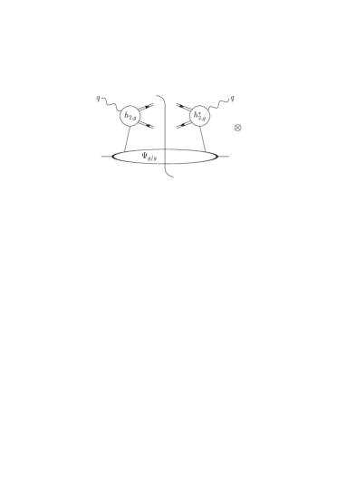
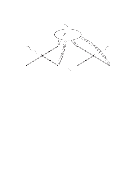
Figure 1: Factorization of heavy quark electroproduction near threshold. The double lines denote eikonal propagators.

At fixed $S_{4}$ the infrared-regulated, differential partonic structure function factorizes [9] as

$$s^{\prime 2}\frac{d^{2}F_{2,g}(x,S_{4},t_{1},u_{1},Q^{2},m^{2})}{dt_{1}\,du_{1}} = H_{2,g}(t_{1},u_{1},Q^{2},m^{2})\;\int dw_{1}dw_{S}$$

$$\times\delta\left({S_{4}\over m^{2}}-w_{1}\Big{(}{-u_{1}\over m^{2}}\Big{)}-w_{S}\right)\;\psi_{g/g}(w_{1},p,\zeta,n)\;S(w_{S},\beta_{i},\zeta,n)\,,$$

where the kinematics relation (12) is implemented in the $\delta$-function. The $\beta_{i}$ are the four-velocities of the particles in the Born approximation to Eq. (7), i.e. with $X[\overline{\rm{Q}}](p_{2}^{\prime})$ replaced by $\overline{\rm{Q}}(p_{2})$. The various functions are computed in $n\cdot A=0$ gauge.

Further manipulations are carried out most conveniently in terms of Laplace moments, defined by

$${\tilde{f}}(N)=\int\limits_{0}^{\infty}dw\,e^{-Nw}f(w)\,.$$ (14)

The upper limit of this integral is not so important, and may also be put at 1, where $\ln w=0$.

As both the gauge and kinematics vector are timelike, we may choose $n^{\mu}=\zeta^{\mu}$, in which case the 1PI $\psi_{i/i}$ are equal to the center-of-mass densities (for which $\zeta^{\mu}=n^{\mu}=\delta^{\mu 0}$) [12].

Replacing the incoming proton with an incoming gluon in Eq. (6) and comparing with Eq. (2), we derive

$$\tilde{\omega}_{2,g}\left(N,{t_{1}\over\mu^{2}},{u_{1}\over\mu^{2}},{Q^{2}\over\mu^{2}},{m^{2}\over\mu^{2}}\right) = H_{2,g}\left({t_{1}\over\mu^{2}},{u_{1}\over\mu^{2}},{Q^{2}\over\mu^{2}},{m^{2}\over\mu^{2}}\right)\;$$ (15)

$$\times \left[{{\tilde{\psi}}_{g/g}(N\left(-u_{1}/m^{2}\right),(p\cdot\zeta/\mu))\over{\tilde{\phi}}_{g/g}(N\left(-u_{1}/m^{2}\right),\mu)}\right]\;{\tilde{S}}({m\over N\mu},\zeta,\beta_{i})\;.$$

Given the factorization in Eqs. (2) and (15), the arguments of [9, 18] ensure that the $N$-dependence in each of the functions of Eq. (15) exponentiates.

We next discuss each function in Eq. (2), or (15), in turn, starting with the $\psi_{g/g}$ wavefunction. In analogy with the center-of-mass definitions [18, 10] it may be defined as an operator matrix element

$$\psi_{g/g}(w,p,\zeta,n) = {1\over 2(N_{c}^{2}-1)}{p\cdot\zeta\over 4\pi(v\cdot p)^{2}}\int\limits_{-\infty}^{\infty}dy\,e^{-iy\,(1-w)p\cdot\zeta}$$ (16)

$$\times \langle g(p)|F^{\mu\,\perp}(y\zeta)\;\Big{[}v_{\mu}v_{\nu}\Big{]}F^{\perp\,\nu}(0)|g(p)\rangle_{n\cdot A=0}\,,$$

where $w=1-z$ and $v_{\mu}$ is a fixed lightlike four-vector in the opposite direction as $p_{\mu}$, such that $v\cdot p$ is of order one. The first factor refers to a spin and color average. The states are normalized such that $\langle 0|A^{\perp}(0)|g(p)\rangle=\epsilon^{\perp}(p)$. Expression (16) as a whole is normalized such that

$$\psi_{g/g}^{(0)}(w) = \delta(w)\,.$$ (17)

We have calculated the order $\alpha_{s}$ corrections to this operator matrix element in general axial gauge $n\cdot A=0$. The $O(\alpha_{s})$ corrections to the operator matrix element in (16) are in $d=4-2\epsilon$ dimensions, and to next-to-leading logarithmic accuracy

$$\psi_{g/g}^{(1)}(w,{p\cdot\zeta\over\mu},\epsilon) = \frac{\alpha_{s}(\mu)}{\pi}\,C_{A}\Bigg{\{}\frac{-1}{\bar{\epsilon}}\left[\frac{1}{w}\right]_{+}+\left[\frac{2\ln(w)}{w}\right]_{+}$$ (18)

$$+\left[\frac{1}{w}\right]_{+}\left(\ln\left(\frac{s}{\mu^{2}}\right)-1+\ln(2\nu_{g})\right)+O(\epsilon)\Bigg{\}}\,,$$

where $\nu_{g}=(\beta_{g}\cdot n)^{2}/|n|^{2}$, with $n^{\mu}$ chosen equal to $\zeta^{\mu}$, and $\beta^{\mu}_{g}$ the four-velocity of the incoming gluon, defined by $p^{\mu}=\beta_{g}^{\mu}\sqrt{s/2}$. Note that $\ln(2\nu_{g})+\ln(s/\mu^{2})=\ln(4(p\cdot\zeta)^{2}/\mu^{2})$. We have abbreviated $1/\bar{\epsilon}=1/\epsilon-\gamma_{E}+\ln 4\pi$. We have verified that the steps for the resummation of the Sudakov double logarithms $\ln^{2}(N)$ in this function trace exactly those for the center-of-mass density introduced for the Drell-Yan process in Ref. [18].

We choose for $\phi_{g/g}$ the $\overline{\rm MS}$ density, which does not have Sudakov double logarithms. To the same accuracy as $\psi_{g/g}$ in Eq. (18), it is given by

$$\phi_{g/g}\left(w,\alpha_{s}(\mu),\epsilon\right) = \delta(w)+\frac{\alpha_{s}(\mu)}{\pi}\,C_{A}\left(\frac{-1}{\bar{\epsilon}}\right)\left[\frac{1}{w}\right]_{+}\,.$$ (19)

The resummation of the singular contributions to this function is done via the Altarelli-Parisi equation [20], see also [9, 21]. We only need this result in combination with the resummed $\psi_{g/g}$ as the ratio $\tilde{\psi}_{g/g}/\tilde{\phi}_{g/g}$ in Eq. (15). This ratio is finite, as can readily be verified at one-loop from Eqs. (18) and (19).

The scale dependence of these functions may be found as follows [10]. The scale dependence of $\tilde{\psi}_{g/g}$ is governed by

$$\mu\frac{d}{d\mu}\ln\tilde{\psi}_{g/g}\left(N,\frac{p\cdot\zeta}{\mu},\alpha_{s}(\mu),\epsilon\right)=\gamma_{\psi}\left(\alpha_{s}(\mu)\right)\,.$$ (20)

The anomalous dimension on the right does not depend on the moment $N$, as the only ultraviolet divergences are due to gluon wavefunction renormalization. Hence, $\gamma_{\psi}=2\gamma_{g}$, where $\gamma_{g}$ is the anomalous dimension of the gluon field in axial gauge.

The anomalous dimension of the $\overline{\rm MS}$ density does depend on $N$, via the Altarelli-Parisi equation

$$\mu\frac{d}{d\mu}\ln\tilde{\phi}_{g/g}(N,\alpha_{s}(\mu),\epsilon)=2\gamma_{g/g}\left(N,\alpha_{s}(\mu)\right)\,.$$ (21)

We next discuss the soft function ${\tilde{S}}(N,\zeta)$. It summarizes the singular contributions arising from soft gluons that are not collinear to the incoming jet, and is infrared finite. It depends on the kinematics of the hard scattering and contributes only at next-to-leading logarithm. Threshold resummation for soft functions is treated in detail in Refs. [11, 16]; a brief sketch will suffice here. The factorization in Eq. (2) introduces ultraviolet divergences, distributed in such a way between the hard function $H$ and the soft function $S$, that they cancel in the product [9, 10]. The function $S$ may be defined as the matrix element of a composite operator that connects Wilson lines in the directions of the external partons. Its extra ultraviolet divergences are cancelled by the renormalization of this operator. As a result, ${\tilde{S}}$ obeys the renormalization group equation

$$\left(\mu{\partial\over\partial\mu}+\beta(\alpha_{s}){\partial\over\partial\,\alpha_{s}}\right)\,{\tilde{S}}=-\left(2{\rm Re}\left\{\Gamma_{S}(\alpha_{s}(\mu))\right\}\right){\tilde{S}}\,,$$ (22)

then resums the $\ln(N)$ terms in $\tilde{S}$. In the reaction under study the anomalous dimension is a $1\,\times\,1$ matrix in color space, so we may solve Eq. (22) directly:

$${\tilde{S}}\left({m\over N\mu},\alpha_{s}(\mu)\right)={\tilde{S}}\left({m\over\mu},\alpha_{s}\left({\mu\over N}\right)\right)\;\exp\left[\,\int\limits_{\mu}^{\mu/N}{d\mu^{\prime}\over\mu^{\prime}}2{\rm Re}\left\{\Gamma_{S}(\alpha_{s}(\mu^{\prime}))\right\}\right]\,.$$ (23)

The resummed hard part may now be written in moment space as

$$\tilde{\omega}_{2,g}\left(N,{t_{1}\over\mu^{2}},{u_{1}\over\mu^{2}},{Q^{2}\over\mu^{2}},{m^{2}\over\mu^{2}}\right) = H_{2,g}\left({t_{1}\over\mu^{2}},{u_{1}\over\mu^{2}},{Q^{2}\over\mu^{2}},{m^{2}\over\mu^{2}}\right)\;{\tilde{S}}\left({m\over\mu},\alpha_{s}\left({\mu\over N}\right)\right)\;$$ (24)

$$\times\;\exp\Bigg{\{}E_{(g)}\Big{(}N\left(\frac{-u_{1}}{m^{2}}\right),m^{2}\Big{)}\Bigg{\}}\exp\Bigg{\{}-2\int\limits_{\mu}^{{m}}{d\mu^{\prime}\over\mu^{\prime}}\left(\gamma_{g}\left(\alpha_{s}(\mu^{\prime})\right)-\gamma_{g/g}\Big{(}N\left(\frac{-u_{1}}{m^{2}}\right),\alpha_{s}(\mu^{\prime})\Big{)}\right)\Bigg{\}}$$

$$\times\;\exp\Bigg{\{}\int\limits_{\mu}^{{{{\mu/N}}}}{d\mu^{\prime}\over\mu^{\prime}}2\,{\rm Re}\left\{\Gamma_{S}\left(\alpha_{s}(\mu^{\prime})\right)\right\}\Bigg{\}}\,.$$

The first exponent summarizes the $N$-dependence of the wave function ratio $\tilde{\psi}_{g/g}/\tilde{\phi}_{g/g}$ and is, in moment space, the same as for heavy quark and dijet production [10, 11]

$$E_{(g)}\left(N_{u},m^{2}\right) = \int\limits^{\infty}_{0}dw\,\frac{(1-e^{-N_{u}w})}{w}\;\Bigg{\{}\int\limits^{1}_{w^{2}}\frac{d\lambda}{\lambda}A_{(g)}\left[\alpha_{s}(\sqrt{\lambda}m)\right]\,$$ (25)

$$+\frac{1}{2}\nu_{(g)}\left[\alpha_{s}(w\,m)\right]\,\Bigg{\}}\,,$$

$$\nu_{(g)} = 2C_{A}\frac{\alpha_{s}}{\pi}\Biggl{\{}1-\ln\left(\frac{4(p\cdot\zeta)^{2}}{m^{2}}\right)\Biggr{\}}\,,$$ (26)

where $N_{u}\equiv N(-u_{1}/m^{2})$, and $A_{(g)}$ is given by the expression

$$A_{(g)}(\alpha_{s})=C_{A}\left({\alpha_{s}\over\pi}+\frac{1}{2}K\left({\alpha_{s}\over\pi}\right)^{2}\right)\,,$$ (27)

with $K=C_{A}\;\left({67/18}-{\pi^{2}/6}\right)-{5/9}n_{f}$ [22] and $n_{f}$ the number of quark flavors.

The second exponent controls the factorization scale dependence of the ratio $\tilde{\psi}_{g/g}/\tilde{\phi}_{g/g}$ through the anomalous dimensions $\gamma_{g}$ and $\gamma_{g/g}$. In axial gauge we find them to be

$$\gamma_{g}\left(\alpha_{s}(\mu)\right) = b_{2}\,\frac{\alpha_{s}(\mu)}{\pi}\,,$$ (28)

$$\gamma_{g/g}\left(N_{u},\alpha_{s}(\mu)\right) = -\frac{\alpha_{s}(\mu)}{\pi}\left(C_{A}{\rm{ln}}(N_{u})-b_{2}\right)+{\cal O}(1/N)\,.$$ (29)

where $b_{2}=(11C_{A}-2n_{f})/12$.

Finally, the $O(\alpha_{s})$ expression for the soft anomalous dimension $\Gamma_{S}$ can be inferred from the UV divergences of the eikonal Feynman graphs in Fig. 2.

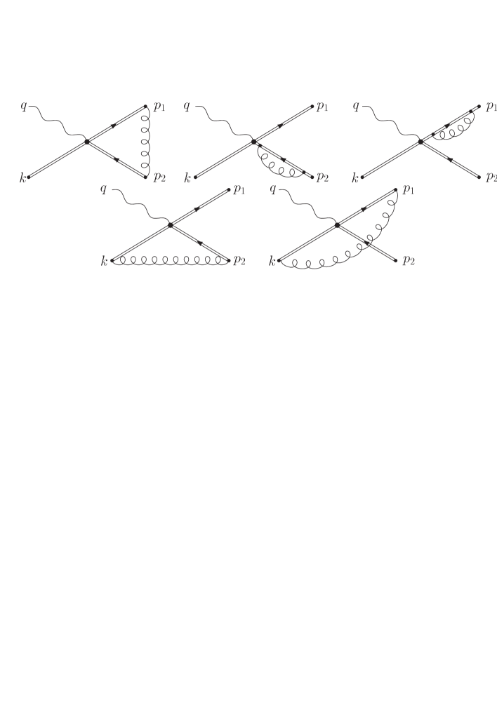
Figure 2: One-loop corrections to the soft function $S$ for heavy-quark production in photon-gluon fusion. The double lines denote eikonal propagators. The lines labelled $k$ corresponds to a gluonic eikonal line, and those labelled $p_{1}$ and $p_{2}$ denote quark and antiquark eikonal lines, respectively.

We obtain the result

$$\Gamma_{S} = \frac{\alpha_{s}}{\pi}\,\Biggl{\{}C_{F}\left(-L_{\beta}-1\right)$$ (30)

$$\hskip 14.22636pt-\,\frac{C_{A}}{2}\left(\ln\left(\frac{4(p\cdot\zeta)^{2}}{m^{2}}\right)-L_{\beta}-1-\ln\left(\frac{-t_{1}}{m^{2}}\right)-\ln\left(\frac{-u_{1}}{m^{2}}\right)\right)\Biggr{\}}\,.$$

where $L_{\beta}$ is given by

$$L_{\beta} = \frac{1-2\,m^{2}/s}{\beta}\left\{\ln\left(\frac{1-\beta}{1+\beta}\right)+{\rm{i}}\pi\right\}\,,\;\;\,\,\,\,\,\beta=\sqrt{1-4m^{2}/s}\,,$$ (31)

and, for single-particle inclusive kinematics,

$$\frac{2p\cdot\zeta}{m}=\frac{-u_{1}}{m^{2}}\,.$$ (32)

At the conclusion of this section a few remarks are in order. First, the integral in the exponent in Eq. (25) can only be interpreted in a formal sense, as some prescription should be implemented to avoid integration over the Landau pole in the running coupling. We do not address such renormalon ambiguities here. In this paper we only employ the resummed expressions as generating functionals of approximate perturbation theory.

Second, although our main focus is on 1PI kinematics, it is straightforward [12] to derive from Eq. (24) the resummed expression for pair-invariant mass kinematics, i.e. the resummed cross section for the process in Eqs. (1) and (7), differential in the ${\rm Q\overline{Q}}$ invariant mass. We present this derivation in appendix B.

3 Finite order results

In this section we expand our resummed cross section to one and two loop order so as to compare with exact NLO calculations [4, 6] and provide NNLO approximations.

We begin by deriving NLL analytic formulae for the single-particle inclusive, partonic hard part $\omega_{2,g}$. Subsequently we study their behavior in the hadronic inclusive structure function $F_{2}^{\rm charm}$, and in the differential distribution $dF_{2}^{\rm charm}/dp_{T}$.

3.1 Partonic results at NLO and NNLO

The Born level hard part (see e.g. [3, 4]) for the process $\gamma^{*}+g\longrightarrow{\rm{Q}}+\overline{\rm{Q}}$ is

$$\omega_{2,g}^{(0)}(s^{\prime},t_{1},u_{1}) = \delta(s^{\prime}+t_{1}+u_{1})\,\sigma^{\rm Born}_{2,g}(s^{\prime},t_{1},u_{1})\,,$$ (33)

with $\sigma^{\rm Born}_{2,g}$ given by

$$\sigma^{\rm Born}_{2,g}(s^{\prime},t_{1},u_{1}) = {\alpha_{s}\over 2\pi}e_{q}^{2}\,{N_{c}C_{F}\over N_{c}^{2}-1}\,Q^{2}\Biggl{[}\frac{t_{1}}{u_{1}}+\frac{u_{1}}{t_{1}}+4\,\frac{m^{2}s^{\prime}}{t_{1}\,u_{1}}\left(1-\frac{m^{2}s^{\prime}}{t_{1}\,u_{1}}\right)$$

$$+ \,2\,\frac{s^{\prime}q^{2}}{t_{1}\,u_{1}}+2\frac{q^{4}}{t_{1}\,u_{1}}+2\,\frac{m^{2}q^{2}}{t_{1}\,u_{1}}\left(2-\frac{s^{\prime\,2}}{t_{1}\,u_{1}}\right)+\frac{12q^{2}}{s^{\prime}}\left(\frac{m^{2}s^{\prime}}{t_{1}\,u_{1}}-\frac{s}{s^{\prime}}\right)\Biggr{]}\,.$$

We now derive the NLO soft gluons corrections to $\omega_{2,g}(s^{\prime},t_{1},u_{1})$ by expanding the resummed hard part in Eq. (24) to one loop, using the explicit expressions for the various functions in Eq. (24), given in Eqs. (18), (19) and (27)-(31). We find

$$\omega_{2,g}^{(1)}(s^{\prime},t_{1},u_{1})~{}\simeq~{}K^{(1)}\,\sigma^{\rm Born}_{2,g}(s^{\prime},t_{1},u_{1})\,,$$ (35)

where

$$K^{(1)} = \frac{1}{-u_{1}}\,\left(\psi_{\rm{g/g}}^{(1)}(w_{1},\epsilon)-\phi_{\rm{g/g}}^{(1)}(w_{1},\epsilon)\right)\Biggr{|}_{w_{1}=s_{4}/(-u_{1}),\epsilon\rightarrow 0}+\frac{1}{m^{2}}\left[\frac{1}{w_{S}}\right]_{+}\,2\,{\rm{Re}}\left\{\Gamma_{S}\right\}\Biggr{|}_{w_{S}=s_{4}/m^{2}}$$ (37)

$$= \frac{\alpha_{s}(\mu)}{\pi}\,\Biggl{[}\,2\,C_{A}\,\left[{\ln(s_{4}/m^{2})\over s_{4}}\right]_{+}+\,\left[{1\over s_{4}}\right]_{+}\Biggl{\{}C_{A}\left(\ln\left(\frac{t_{1}}{u_{1}}\right)+{\rm{Re}}L_{\beta}-\ln\left(\frac{\mu^{2}}{m^{2}}\right)\right)$$

$$\hskip 113.81102pt-2\,C_{F}\left({\rm{Re}}L_{\beta}+1\right)\Biggr{\}}+\,\delta(s_{4})\,C_{A}\ln\left(\frac{-u_{1}}{m^{2}}\right)\ln\left(\frac{\mu^{2}}{m^{2}}\right)\,\Biggr{]}\,,$$

with $\mu$ the $\overline{{\rm{MS}}}$-mass factorization scale and $L_{\beta}$ given in Eq. (31). The plus-distributions in $s_{4}$ have been defined in Eq. (10). To next-to-leading logarithm, the result in Eq. (37) agrees with the exact $\alpha_{s}$ corrections of Ref. [4]. This holds for the contributions both independent and dependent on the factorization scale, i.e. terms including powers of $\ln(\mu/m)$.

The scale-dependent logarithms $\ln(\mu/m)$ are explicitly generated by the second exponent in Eq. (24), involving the anomalous dimensions $\gamma_{g}$ and $\gamma_{g/g}$ given in Eqs. (28) and (29). In deriving $\gamma_{g/g}$ in Eq. (29) we have carefully determined all terms which are constant in moment space, including the $\ln(-u_{1}/m^{2})$ logarithm, absorbed in $N_{u}$. In this way we are able to determine all factorization scale dependent terms to NLL accuracy.

The NNLO corrections may be found in a manner exactly analogous to what was done for Drell-Yan in Ref. [23] and for Higgs production in Ref. [21]. We expand Eq. (24) to second order in $\alpha_{s}$ in moment space. With the table of Laplace transforms in appendix A for the singular distributions in Eq. (10), we then find the ${\cal O}(\alpha_{s}^{2})$ threshold-enhanced corrections in momentum space. Our result is

$$\omega_{2,g}^{(2)}(s^{\prime},t_{1},u_{1})~{}\simeq~{}K^{(2)}\,\sigma^{\rm Born}_{2,g}(s^{\prime},t_{1},u_{1})\,,$$ (38)

with

$$\displaystyle K^{(2)} = \frac{\alpha^{2}_{s}(\mu)}{\pi^{2}}\,\Biggl{[}\,2\,C_{A}^{2}\,\left[{\ln^{3}(s_{4}/m^{2})\over s_{4}}\right]_{+}$$

$$\hskip 11.38109pt\displaystyle+\,\left[{\ln^{2}(s_{4}/m^{2})\over s_{4}}\right]_{+}\Biggl{\{}3\,C_{A}^{2}\,\left(\ln\left(\frac{t_{1}}{u_{1}}\right)+{\rm{Re}}L_{\beta}-\ln\left(\frac{\mu^{2}}{m^{2}}\right)\right)$$

$$\hskip 42.67912pt-2\,C_{A}\left(b_{2}+3\,C_{F}\left({\rm{Re}}L_{\beta}+1\right)\right)\Biggr{\}}$$

$$\hskip 11.38109pt+\,\left[{\ln(s_{4}/m^{2})\over s_{4}}\right]_{+}\ln\left(\frac{\mu^{2}}{m^{2}}\right)\left\{C_{A}^{2}\,\left(-2\ln\left(\frac{t_{1}}{u_{1}}\right)-2{\rm{Re}}L_{\beta}+2\ln\left({-u_{1}\over m^{2}}\right)+\ln\left(\frac{\mu^{2}}{m^{2}}\right)\right)\right.$$

$$\hskip 42.67912pt+2\,C_{A}\,\left(b_{2}+2\,C_{F}\left({\rm{Re}}L_{\beta}+1\right)\right)\Biggr{\}}$$

$$\hskip 11.38109pt+\,\left[{1\over s_{4}}\right]_{+}\ln^{2}\left(\frac{\mu^{2}}{m^{2}}\right)\left\{-C_{A}^{2}\ln\left({-u_{1}\over m^{2}}\right)\,-\frac{1}{2}\,C_{A}\,b_{2}\right\}\,\Biggr{]}\,.$$

and $b_{2}=(11C_{A}-2n_{f})/12$.

3.2 Gluon coefficient functions

The inclusive structure function $F_{2,P}^{\rm charm}$ is obtained from Eq. (6) by integrating over $T_{1}$ and $U_{1}$. It can be expanded in coefficient functions $c^{(k,l)}_{2,g}$ as follows (dropping the $P$ subscript)

$$F_{2}^{\rm charm}(x,Q^{2},m^{2})\! = \!\frac{\alpha_{s}(\mu)\,e_{{\rm c}}^{2}Q^{2}}{4\pi^{2}m^{2}}\!\int\limits_{ax}^{1}\,dz\,\phi_{g/P}(z,\mu^{2})\,\sum\limits_{k=0}^{\infty}(4\pi\alpha_{s}(\mu))^{k}\sum\limits_{l=0}^{k}c^{(k,l)}_{2,g}(\eta,\xi)\ln^{l}\frac{\mu^{2}}{m^{2}},\,\,\,\,\,$$ (40)

where $a=(Q^{2}+4m^{2})/Q^{2}$ and we recall that contributions from light initial state quarks are neglected. The function $\phi_{g/P}(z,\mu^{2})$ denotes the gluon PDF and the functions $c^{(k,l)}_{2,g}$ depend on the scaling variables

$$\eta = \frac{s}{4m^{2}}\,-1\,,\,\,\,\,\,\,\,\,\,\,\,\,\,\,\,\,\,\,\xi\,=\,\frac{Q^{2}}{m^{2}}\,.$$ (41)

The variable $\eta$ is a direct measure of the distance to the partonic threshold. The inclusive coefficient functions are obtained from Eqs. (37) and (3.1) by

$$c^{(k,l)}_{2,g}(\eta,\xi) = \int\limits_{s^{\prime}(1-\beta)/2}^{s^{\prime}(1+\beta)/2}\,d(-t_{1})\int\limits_{0}^{s_{4}^{\rm max}}\,ds_{4}\,\,\,\frac{d^{2}c^{(k,l)}_{2,g}(s^{\prime},t_{1},u_{1})}{dt_{1}\,ds_{4}}\,,$$ (42)

where the double differential coefficient functions are in turn related to the hard part $\omega_{2,g}$ of Eq. (6) by

$$\sum\limits_{l=0}^{k}s^{\prime 2}\frac{d^{2}c^{(k,l)}_{2,g}(s^{\prime},t_{1},u_{1})}{dt_{1}\,ds_{4}}\ln^{l}\frac{\mu^{2}}{m^{2}}=\frac{4\pi^{2}}{\alpha_{s}e_{c}^{2}(4\pi\alpha_{s})^{k}}\,\frac{m^{2}}{Q^{2}}\,\,\omega^{(k)}_{2,g}(s^{\prime},t_{1},u_{1})\,\Biggr{|}_{u_{1}=s^{\prime}+t_{1}-s_{4}}\,.$$ (43)

Also, in Eq. (42) we abbreviated [4]

$$s_{4}^{\rm max} = \frac{s}{s^{\prime}\,t_{1}}\,\left(t_{1}+\frac{s^{\prime}(1-\beta)}{2}\right)\left(t_{1}+\frac{s^{\prime}(1+\beta)}{2}\right)\,.$$ (44)

We begin our numerical studies with the gluon coefficient functions $c^{(k,0)}_{2,g}(\eta,\xi)$, i.e. those that are not accompanied by scale-dependent logarithms. We recall that all our results are derived in the $\overline{\rm MS}$ scheme. The functions $c^{(0,0)}_{2,g}$ and $c^{(1,0)}_{2,g}$ are known exactly, see Ref. [4]. The one-loop expansion of our resummed hard part provides an approximation to the exactly known $c^{(1,0)}_{2,g}$. To judge the benefits of resumming to next-to-leading logarithmic as compared to leading logarithmic accuracy, we can distill also LL expressions, by keeping only the $[\ln(s_{4}/m^{2})/s_{4}]_{+}$ and $[\ln^{3}(s_{4}/m^{2})/s_{4}]_{+}$ terms in Eqs. (37) and (3.1) respectively.

Figure 3: (a): The $\eta$-dependence of the coefficient functions $c^{(k,0)}_{2,g}(\eta,\xi),\;k=0,1$ for $Q^{2}=0.1\,{\rm GeV}^{2}$ with $m=1.5\,{\rm GeV}$. Plotted are the exact results for $c^{(k,0)}_{2,g},\;k=0,1$ (solid lines), the LL approximation to $c^{(1,0)}_{2,g}$ (dotted line) and the NLL approximation to $c^{(1,0)}_{2,g}$ (dashed line). (b): The $\eta$-dependence of the coefficient function $c^{(2,0)}_{2,g}(\eta,\xi)$ for $Q^{2}=0.1\,{\rm GeV}^{2}$ with $m=1.5\,{\rm GeV}$. Plotted are the LL approximation (dotted line) and the NLL approximation (dashed line).

Figure 4: (a): The $\eta$-dependence of the coefficient functions $c^{(k,0)}_{2,g}(\eta,\xi),\;k=0,1$ for $Q^{2}=10\,{\rm GeV}^{2}$ with $m=1.5\,{\rm GeV}$. The notation is the same as in Fig. 3a. (b): The $\eta$-dependence of the coefficient function $c^{(2,0)}_{2,g}(\eta,\xi)$ for $Q^{2}=10\,{\rm GeV}^{2}$ with $m=1.5\,{\rm GeV}$. The notation is the same as in Fig. 3b.

Figure 5: (a): The NLL approximation to the coefficient function $c^{(1,0)}_{2,g}(\eta,\xi)$ for $Q^{2}=10\,{\rm GeV}^{2}$ and $m=1.5\,{\rm GeV}$ with restrictions to the small $\eta$-region. Plotted are the unmodified NLL result (solid line), the NLL result with a factor $\theta(m^{2}-s_{4})$ included (dotted line) and the NLL result multiplied with a damping factor $1/\sqrt{1+\eta}$ (dashed line). (b): The $\eta$-dependence of the NLL approximation to the coefficient function $c^{(2,0)}_{2,g}(\eta,\xi)$ for $Q^{2}=10\,{\rm GeV}^{2}$ and $m=1.5\,{\rm GeV}$. The notation is the same as in Fig. 5a.

In Figs. 3a and 4a we plot the functions $c^{(k,0)}_{2,g}(\eta,\xi),\;k=0,1$ versus $\eta$, for two values of $\xi=Q^{2}/m^{2}$. For the coefficient functions only the ratio $\xi$ matters, however, we chose those values to correspond to $Q^{2}=0.1$ and $10$ ${\rm GeV}^{2}$ for a charm mass of $m=1.5\,{\rm GeV}$. These figures reveal that, at one loop, the LL accuracy provides a good approximation for very small $\eta$, however, with significant deviations from the exact result for larger $\eta$, i.e. as the distance from threshold increases. On the other hand, the NLL approximation is excellent over a much wider range in $\eta$, up to values of about 10.

We also show $c^{(2,0)}_{2,g}$, obtained from Eqs. (3.1) and (43), in LL and NLL approximation in Figs. 3b and 4b for the same values of $m$ and $Q^{2}$ as before. We observe more structure than in the $c^{(1,0)}_{2,g}$ curves. Figs. 3b and 4b show some sizable deviations from zero at large $\eta$, which leads us to consider the following issue. Kinematically, larger $\eta$ values allow $w=s_{4}/m^{2}\gg 1$, whereas, in contrast, the threshold region is defined by $w\approx 0$. Therefore we should consider the inclusion of a factor $\theta(m^{2}-s_{4})$ in the integral (42) in order to suppress spurious large corrections in the large $\eta$ region.

In Figs. 5a and 5b we show the effect of the veto $\theta(m^{2}-s_{4})$ on the NLL coefficient functions $c^{(k,0)}_{2,g}$ for $k=1,2$ for values of $Q^{2}=10\,{\rm GeV}^{2}$ and $m=1.5\,{\rm GeV}$. Also shown is the effect of a damping factor $1/\sqrt{1+\eta}$ [24], which can be included outside the integral in Eq. (42) and is therefore easier to implement. We see that the effect of the veto is well-mimicked by the damping factor, therefore we shall use the latter, rather than the veto, where needed in what follows. Of course, for smaller values of $\eta$ the damping factor leads to a slight underestimation of the coefficient functions compared to the veto, but these effects are negligible, as Fig. 5 shows.

Figure 6: (a): The $\eta$-dependence of the coefficient function $c^{(1,1)}_{2,g}(\eta,\xi)$ for $Q^{2}=0.1\,{\rm GeV}^{2}$ with $m=1.5\,{\rm GeV}$. Plotted are the exact result (solid line), the LL approximation (dotted line) and the NLL approximation (dashed line). (b): The $\eta$-dependence of the coefficient functions $c^{(2,l)}_{2,g}(\eta,\xi),\;l=1,2$ for $Q^{2}=0.1\,{\rm GeV}^{2}$ with $m=1.5\,{\rm GeV}$. Plotted are the exact results (solid lines), the LL approximations (dotted lines) and the NLL approximations (dashed lines).

Figure 7: (a): The $\eta$-dependence of the coefficient function $c^{(1,1)}_{2,g}(\eta,\xi)$ for $Q^{2}=10\,{\rm GeV}^{2}$ with $m=1.5\,{\rm GeV}$. The notation is the same as in Fig. 6a. (b): The $\eta$-dependence of the coefficient functions $c^{(2,l)}_{2,g}(\eta,\xi),\;l=1,2$ for $Q^{2}=0.1\,{\rm GeV}^{2}$ with $m=1.5\,{\rm GeV}$. The notation is the same as in Fig. 6b.

Figure 8: (a): The NLL approximation to the coefficient function $c^{(1,1)}_{2,g}(\eta,\xi)$ for $Q^{2}=10\,{\rm GeV}^{2}$ and $m=1.5\,{\rm GeV}$ with restrictions to the small $\eta$-region. The notation is the same as in Fig. 5a (b): The NLL approximation to the coefficient function $c^{(2,l)}_{2,g}(\eta,\xi),\,l=1,2$ for $Q^{2}=10\,{\rm GeV}^{2}$ and $m=1.5\,{\rm GeV}$ with restrictions to the small $\eta$-region. The notation is the same as in Fig. 5a.

Let us now investigate those coefficient functions $c^{(k,l)}_{2,g}(\eta,\xi),\,l\geq 1$ in Eq. (40) that determine the dependence of $F_{2}^{\rm charm}$ on the mass factorization scale $\mu$. As mentioned earlier, this is of some relevance since the exact NLO $F_{2}^{\rm charm}$ exhibits considerably more $\mu$ sensitivity at large $x$ (near threshold), than at small $x$, cf. Ref. [8]. The natural question arises whether and, if so how much, our approximate NNLO results might improve the situation.

Explicitly, the coefficient functions under consideration up to NNLO are $c^{(1,1)}_{2,g}$ which is known exactly [4] and the previously unknown functions $c^{(2,1)}_{2,g}$ and $c^{(2,2)}_{2,g}$. We can infer the exact results for these functions from renormalization group arguments. We find

$$c^{(1,1)}_{2,g} = \frac{1}{4\pi^{2}}\left[b_{2}\,c^{(0,0)}_{2,g}-\frac{1}{2}c^{(0,0)}_{2,g}\otimes P_{gg}^{(0)}\right]\,,$$ (45)

$$c^{(2,1)}_{2,g} = \frac{1}{(4\pi^{2})^{2}}\left[b_{3}\,c^{(0,0)}_{2,g}-\frac{1}{2}c^{(0,0)}_{2,g}\otimes P_{gg}^{(1)}\right]\,+\frac{1}{4\pi^{2}}\left[2b_{2}\,c^{(1,0)}_{2,g}-\frac{1}{2}c^{(1,0)}_{2,g}\otimes P_{gg}^{(0)}\right]\,,$$ (46)

$$c^{(2,2)}_{2,g} = \frac{1}{(4\pi^{2})^{2}}\left[b_{2}^{2}\,c^{(0,0)}_{2,g}-\frac{3}{4}b_{2}\,c^{(0,0)}_{2,g}\otimes P_{gg}^{(0)}+\frac{1}{8}c^{(0,0)}_{2,g}\otimes P_{gg}^{(0,0)}\right]\,,$$ (47)

with $\beta$-function coefficients $b_{2}=(11C_{A}-2n_{f})/12$, $b_{3}=(34C_{A}^{2}-6C_{F}n_{f}-10C_{A}n_{f})/48$ and the one- and two-loop gluon-gluon splitting functions $P_{gg}^{(0)}$, $P_{gg}^{(1)}$, cf. Ref. [25]. The convolutions involving a coefficient function $c^{(i,0)}_{2,g}$ are defined as

$$\left(c^{(i,0)}_{2,g}\otimes P_{gg}^{(j)}\right)(\eta(x),\xi) \equiv \int\limits_{ax}^{1}\,dz\,\,c^{(i,0)}_{2,g}\left(\eta\left(\frac{x}{z}\right),\xi\right)\,P_{gg}^{(j)}(z)\,,$$ (48)

where $a=(Q^{2}+4m^{2})/Q^{2}$ and $\eta(x)$ is derived from Eq. (41), $\eta(x)=\xi/4(1/x-1)-1$. Finally, the function $P_{gg}^{(0,0)}$ in Eq. (47) is given by the standard convolution of two splitting functions $P_{gg}^{(0)}$,

$$P_{gg}^{(0,0)}(x) \equiv \int\limits_{0}^{1}\,dx_{1}\,\int\limits_{0}^{1}\,dx_{2}\,\delta(x-x_{1}x_{2})P_{gg}^{(0)}(x_{1})P_{gg}^{(0)}(x_{2})\,.$$ (49)

With Eqs. (45)-(47) in hand, we are able to check the quality of our NLL approximation at NLO and NNLO against exact answers. Again, to fully appreciate the improvement of NLL resummation, we truncate our approximation to LL accuracy, keeping only the $\ln(\mu/m)[1/s_{4}]_{+}$ term in Eq. (37) and the terms $\ln(\mu/m)[\ln^{2}(s_{4}/m^{2})/s_{4}]_{+}$ and $\ln^{2}(\mu/m)[\ln(s_{4}/m^{2})/s_{4}]_{+}$ in Eq. (3.1), respectively.

In Figs. 6a and 7a we plot the function $c^{(1,1)}_{2,g}(\eta,\xi)$ versus $\eta$, for two values of $\xi=Q^{2}/m^{2}$, while Figs. 6b and 7b display the functions $c^{(2,l)}_{2,g},\;l=1,2$. The evaluation of Eq. (46) has been performed with the help of the parametrization for $c^{(1,0)}_{2,g}$ from Ref. [26]. From Figs. 6 and 7, we see again that the NLL approximations are superior to the LL ones. In Figs. 8a and 8b we show the effect of the veto $\theta(m^{2}-s_{4})$ in the integral (42) and the damping factor $1/\sqrt{1+\eta}$ on $c^{(1,1)}_{2,g}(\eta,\xi)$ and $c^{(2,l)}_{2,g}(\eta,\xi),\,l=1,2$ for values of $\xi$ corresponding to $Q^{2}=10\,{\rm GeV}^{2}$ and $m=1.5\,{\rm GeV}$. In the following sections we shall for the sake of uniformity include a damping factor for the $c^{(2,l)}_{2,g}(\eta,\xi),\,l=1,2$ and $c^{(1,1)}_{2,g}(\eta,\xi)$, even though the undamped NLL $c^{(1,1)}_{2,g}$ approximates the exact $c^{(1,1)}_{2,g}$ somewhat better, as a comparison of Figs. 7a and 8a shows. We verified that the difference is negligible at the hadronic level.

3.3 Inclusive structure function $F_{2}^{\rm charm}$

Having obtained encouraging results for the quality of the partonic approximations Eqs. (37) and (3.1) at the inclusive level, we shall now assess their effect at the hadronic level.

Throughout we use the CTEQ4M [27] gluon density. For NLO plots we use the two-loop expression for $\alpha_{s}$ with $n_{f}=4$, $\Lambda=0.298\,{\rm GeV}$. Respectively, for NNLO plots, the three-loop expression [28] for $\alpha_{s}$ and an adjusted $\Lambda=0.265\,{\rm GeV}$.

In Fig. 9a and 9b we plot the gluon density $\phi_{g/P}(x/z,\mu^{2})$ as a function of $\eta$ on the same scale as the coefficient functions $c^{(k,l)}_{2,g}(\eta,\xi)$ for $x=0.1$ and $0.01$ and three different choices of the factorization scale ($\mu=m,2m,\sqrt{Q^{2}+4m^{2}}$). From now on we use a charm mass of $m=1.6\,{\rm GeV}$ and take $Q^{2}=10\,{\rm GeV}$. Our heavy quark mass is always a pole mass, as in Ref. [4]. The figure shows that the gluon density indeed provides support for the coefficient functions in Eq. (40) in the threshold region for $x\geq 0.01$, although the figure also shows the extent of the support to be somewhat scale sensitive.

Figure 9: (a): The CTEQ4M gluon density $\phi_{g/P}(x/z,\mu^{2})$ as a function of $\eta$ for $m=1.6\,{\rm GeV}$, $Q^{2}=10\,{\rm GeV}$ and $x=0.1$. Plotted are the scale choice $\mu=m$ (solid line), $\mu=2m$ (dashed line) and $\mu=\sqrt{Q^{2}+4m^{2}}$ (dotted line). (b): Same as Fig. 9a for $x=0.01$.

A more revealing way to examine the support of the gluon density in Eq. (40) is to plot the integral as a function of $z_{\rm{max}}$,

$$F_{2}^{\rm charm}(x,Q^{2},m^{2},z_{\rm{max}})\! \simeq \!\frac{\alpha_{s}(\mu)\,e_{{\rm c}}^{2}Q^{2}}{4\pi^{2}m^{2}}\!\int\limits_{ax}^{z_{\rm{max}}}\,dz\,\phi_{g/P}(z,\mu^{2})\,\sum\limits_{k=0}^{\infty}(4\pi\alpha_{s}(\mu))^{k}\sum\limits_{l=0}^{k}c^{(k,l)}_{2g}(\eta,\xi)\ln^{l}\frac{\mu^{2}}{m^{2}}\,.\,\,\,\,\,\,\,\,\,\,\,\,$$ (50)

Varying the theoretical cut-off $z_{\rm{max}}$ allows us see where the integral (50) acquires most of its value. The physical structure function corresponds to ${z_{\rm{max}}}=1$.

In Figs. 10a and 10b we show the results for the numerical evaluation of Eq. (50) and compare to the exact NLO calculation of Ref. [4] for two values of $x=0.1,0.01$ and two choices of the factorization scale $\mu=m,\sqrt{Q^{2}+4m^{2}}$. The scale dependent terms in the NLL approximation to Eq. (50) have been multiplied with a damping factor $1/\sqrt{1+\eta}$ in order to suppress spurious contributions from the large $\eta$ region, i.e. far above partonic threshold.

Figs. 10a and 10b show that, for the chosen kinematical range in $x$ and $Q^{2}$, $F_{2}^{\rm charm}$ as defined by Eq. (50) originates entirely from that region in $\eta$ in which we approximate the exact results very well. In words, for the values of $x$ shown, $F_{2}^{\rm charm}$ is completely determined by partonic processes close to threshold. We observe that the NLL approximation to Eq. (50) is much better than the LL one at the hadronic level as well. As we shall shortly show in more detail, it is also significantly more stable under variations of the factorization scale.

Figure 10: (a): $F_{2}^{\rm charm}(x,Q^{2},z_{\rm{max}})$ as a function of $z_{\rm{max}}$ at NLO with the CTEQ4M gluon PDF, $x=0.1$, $m=1.6\,{\rm GeV}$, $Q^{2}=10\,{\rm GeV}$ and $\mu=m$ (upper three curves), $\mu=\sqrt{Q^{2}+4m^{2}}$ (lower three curves). Plotted are: The exact results (solid lines), the LL approximations (dotted lines) and the NLL approximations with the damping factor $1/\sqrt{1+\eta}$ on the scale dependent terms only (dashed lines). (b): Same as Fig. 10a for $x=0.01$. The lower three curves, $\mu=\sqrt{Q^{2}+4m^{2}}$, have been scaled down by a factor of 2.

Figure 11: (a): $F_{2}^{\rm charm}(x,Q^{2},z_{\rm{max}})$ as a function of $z_{\rm{max}}$ at NNLO in NLL approximation with the CTEQ4M gluon PDF, $x=0.1$, $m=1.6\,{\rm GeV}$, $Q^{2}=10\,{\rm GeV}$ and with the damping factor $1/\sqrt{1+\eta}$ on all scale dependent terms and on $c^{(2,0)}_{2,g}$. Plotted are: Scale choices $\mu=m$ (upper curve) and $\mu=\sqrt{Q^{2}+4m^{2}}$ (lower curve). (b): Same as Fig. 11a for $x=0.01$. Plotted are: Scale choices $\mu=m$ (lower curve) and $\mu=\sqrt{Q^{2}+4m^{2}}$ (upper curve).

In Figs. 11a and 11b we display the results for Eq. (50) evaluated to NNLO in NLL approximation for the same kinematical values and choices for $\mu$ as before. Again, we have multiplied the NLO scale dependent terms $c^{(1,1)}_{2,g}$ and also all NNLO terms $c^{(2,l)}_{2,g}\,,l=0,1,2$ with a damping factor $1/\sqrt{1+\eta}$. Figs. 11a and 11b reveal that the NNLO corrections are numerically quite sizable. However, the variations with respect to the mass factorization scale are still large for both values of $x=0.1,0.01$.

Let us therefore turn to the issue of factorization scale dependence of the hadronic structure function in more detail. The scale dependence of $F_{2}^{\rm charm}$, cf. Eq.(40), at NLO is exhibited in Figs. 12a and 12b over a range in $m\leq\mu\leq 2\sqrt{Q^{2}+4m^{2}}$. For $x=0.1,0.01$ we compare the exact result of Ref. [4] with the LL and the NLL approximations from Eq. (37). The coefficient $c^{(1,1)}_{2,g}$ is in the approximations again multiplied by the damping factor $1/\sqrt{1+\eta}$.

Figure 12: (a): The $\mu$-dependence of the charm structure function $F_{2}^{\rm charm}$ at NLO with the CTEQ4M gluon PDF, $x=0.1$, $m=1.6\,{\rm GeV}$ and $Q^{2}=10\,{\rm GeV}$. Plotted are: The exact result (solid line), the LL approximation (dotted line) and the NLL approximation with the damping factor $1/\sqrt{1+\eta}$ on the scale dependent terms (dashed line). (b): Same as Fig. 12a for $x=0.01$.

Figure 13: (a): The $\mu$-dependence of the charm structure function $F_{2}^{\rm charm}$ at NNLO with the CTEQ4M gluon PDF, $x=0.1$, $m=1.6\,{\rm GeV}$, $Q^{2}=10\,{\rm GeV}$. Plotted are the improved NLL approximation (dashed line; exact NLO result plus NLL approximate NNLO result with the damping factor $1/\sqrt{1+\eta}$) and the best approximation (solid line; exact results at NLO and for $c^{(2,1)}_{2,g}$ and $c^{(2,2)}_{2,g}$ plus NLL approximation $c^{(2,0)}_{2,g}$ with the damping factor $1/\sqrt{1+\eta}$). (b): Same as Fig. 13a for $x=0.01$.

Figure 14: (a): The $x$-dependence of the charm structure function $F_{2}^{\rm charm}$ at NLO with the CTEQ4M gluon PDF, $\mu=m=1.6\,{\rm GeV}$ and $Q^{2}=10\,{\rm GeV}$. Plotted are: The exact result (solid line), the LL approximation (dotted line) and the NLL approximation (dashed line). (b): The $x$-dependence of the ratios $F_{2\,\,(NLO)}^{\rm charm}/F_{2\,\,(LO)}^{\rm charm}$ (solid line) and $F_{2\,\,(NNLO)}^{\rm charm}/F_{2\,\,(NLO)}^{\rm charm}$ (dashed line) with $F_{2\,\,(NNLO)}^{\rm charm}$ in the improved NLL approximation (exact NLO result plus NLL approximate NNLO result with the damping factor $1/\sqrt{1+\eta}$) and parameter choices as in Fig. 14a.

Figure 15: (a): The $x$-dependence of $F_{2}^{\rm charm}$ at NLO (lower band), scaled down by a factor of 10 and (upper band) in the improved NLL approximation at NNLO (exact NLO result plus NLL approximate NNLO result with the damping factor $1/\sqrt{1+\eta}$) with the CTEQ4M gluon PDF, $\mu=m$, $Q^{2}=10\,{\rm GeV}$. The bands correspond to the charm mass variation $1.35\,{\rm GeV}\leq m\leq 1.7\,{\rm GeV}$. (b): Same as Fig. 10a for $\mu=\sqrt{Q^{2}+4m^{2}}$.

We see from Figs. 12a and 12b that resummation to NLL accuracy is crucial to obtain a reliable behaviour with respect to the $\mu$-dependence of $F_{2}^{\rm charm}$ at NLO. The NLL curve traces the exact result extremely well, in particular at phenomenological interesting smaller $x$ values, when the support of gluon PDF extends to regions of $\eta=1$ to $10$. In fact, Fig. 12b clearly shows that in this kinematical domain, the LL approximation is rather poorly behaved.

Continuing, we display in Figs. 13a and 13b the effect of the NNLO corrections on the scale dependence of $F_{2}^{\rm charm}$. We compare an improved NLL approximation to $F_{2}^{\rm charm}$ at NNLO, which consists of the exact result of Ref. [4] for $F_{2}^{\rm charm}$ at NLO and, additionally, our NLL approximate NNLO results from Eq.(3.1), with the so-called best approximation to $F_{2}^{\rm charm}$ at NNLO. This best approximation extends beyond the NLL accuracy at two-loop order as it contains the full exact results for $c^{(2,1)}_{2,g}$ and $c^{(2,2)}_{2,g}$ from Eqs. (46), (47), such that only $c^{(2,0)}_{2,g}$ remains approximate to NLL accuracy.

We observe practically no improvement, with respect to the NLO result, in the scale dependence of $F_{2}^{\rm charm}$ at large $x$ near threshold (Fig. 13a), where the relative variations with respect to $\mu$ were largest before. We also see here that the two approximations to $F_{2}^{\rm charm}$ at NNLO, the NLL improved and the best, agree very well. They are differing only by terms beyond the NLL accuracy, which turn out to be rather small numerically. Therefore it is also unlikely that any corrections to $c^{(2,0)}_{2,g}$ beyond the NLL accuracy will help to soften the large $\mu$-dependence of $F_{2}^{\rm charm}$ at large $x$.

On the other hand, for smaller $x$ (Fig. 13b), we indeed see an indication of increased NNLO stability. The best NNLO approximation to $F_{2}^{\rm charm}$ reduces the value of the relative variation $F_{2}^{\rm charm}(\mu=m)/F_{2}^{\rm charm}(\mu=2\sqrt{Q^{2}+4m^{2}})$ from 1.13 at NLO to 1.07 at NNLO, so that there is practically no dependence on $\mu$ left. Naturally, for smaller $x$, where one probes regions away from threshold, terms beyond the NLL accuracy also have some numerical importance, as one may see from the difference between the two approximations to $F_{2}^{\rm charm}$ in Fig. 13b. Finally, we note that a fully consistent NNLO scale dependence study would require not-yet-available NNLO parton densities, and the presently also unknown three-loop anomalous dimensions.

The final comparison in this subsection involves the size and $x$ dependence of $F_{2}^{\rm charm}$ at a fixed value of the factorization scale $\mu=m$. In Fig. 14a we compare the exact result of Ref. [4] with the LL and the NLL approximations from Eq. (37), over a range of $x$, $0.003\leq x\leq 0.3$. We find that the deviations of the NLL approximation from the exact result are often very small, at most $10\%$ for the value of $x=0.003$. The excellence of the NLL approximation to the $x$ dependence also holds for other values of $\mu$.

In Fig. 14b we display for the same kinematics and over the same range in $x$ the effect of the NNLO corrections. We plot the K-factors $F_{2\,\,(NNLO)}^{\rm charm}/F_{2\,\,(NLO)}^{\rm charm}$ and, for comparison, also $F_{2\,\,(NLO)}^{\rm charm}/F_{2\,\,(LO)}^{\rm charm}$ . At NNLO we have taken the improved NLL approximation to $F_{2}^{\rm charm}$ (we recall: the exact NLO result plus the NLL approximate NNLO result with the damping factor $1/\sqrt{1+\eta}$). We see that particularly for smaller $x$, the size of the NNLO corrections is negligible, the K-factor being close to one, whereas for larger $x$, their overall size is still quite big, almost a factor of 2 at $x=0.1$.

We note furthermore that the largest error on the approximate NNLO $F_{2}^{\rm charm}$, as at NLO [14], is still due to the uncertainty in the charm mass. Varying the mass of the charm from 1.35 to 1.7 GeV, we found sizeable variations in the absolute value of $F_{2}^{\rm charm}$, in particular a larger $x$. In Figs. 15a and 15b we plot for two values of the factorization scale $\mu$ the improved NLL approximation to $F_{2}^{\rm charm}$ as a function of $x$, $0.003\leq x\leq 0.3$. For comparison, Figs. 15a and 15b also contain the exact NLO result with same variations of the charm mass. In general, decreasing the charm mass increases $F_{2}^{\rm charm}$.

This concludes our investigation of the inclusive structure function $F_{2}^{\rm charm}$.

3.4 $dF_{2}^{\rm charm}/dp_{T}$

In this subsection we study the distribution $dF_{2}^{\rm charm}/dp_{T}$. Soft gluon resummation might be especially fruitful here because the requirement that the detected charm quark has a fixed transverse momentum increases the sensitivity to threshold dynamics by effectively increasing the heavy quark mass from $m$ to the transverse mass $m_{T}=\sqrt{m^{2}+p_{T}^{2}}$.

Eq. (6) provides us with the differential distribution $d^{2}F_{2}/dT_{1}dU_{1}$ from which we can derive the experimentally relevant distribution $d^{2}F_{2}/dydp_{T}$, with $y$ being the rapidity in the c.m. frame of the vitual photon-proton system and $p_{T}$ the transverse momentum of the detected heavy quark. In terms of the Mandelstam variables of Eq. (4), we can write the energy of the outgoing heavy-quark as

$$E = -\,\frac{Q^{2}+T_{1}+U_{1}}{2\,\sqrt{S}}\,.$$ (51)

The transverse momentum $p_{T}$ and the longitundinal momentum $p_{L}$ are determined by

$$S^{\prime\,2}(p_{T}^{2}+m^{2}) = S^{\prime}T_{1}U_{1}+Q^{2}T_{1}^{2}+Q^{2}S^{\prime}T_{1}\,,$$ (52)

$$p_{L}^{2} = E^{2}-m^{2}-p_{T}^{2}\,,$$ (53)

where $S^{\prime}=S+Q^{2}$. The rapidity $y$

$$y = \frac{1}{2}\,\ln\left(\frac{E+p_{L}}{E-p_{L}}\right)\,.$$ (54)

may then be expressed in terms of $(T_{1},U_{1})$ by Eqs. (51) and (53). The transformation $(T_{1},U_{1})\to(p_{T},y)$ is then defined. Neglecting all light initial state quarks, one obtains from Eq. (6) the result for the inclusive distribution $dF_{2}/dp_{T}$,

$$\frac{d^{2}F_{2}(x,p_{T},Q^{2},m^{2})}{dp_{T}} \simeq \frac{2\,p_{T}}{S^{\prime}}\,\int\limits_{y^{-}}^{y^{+}}dy\int\limits_{z^{-}}^{1}\frac{dz}{z}\,\phi_{g/P}(z,\mu^{2})\,\omega_{2,g}\Big{(}{x\over z},s_{4},t_{1},u_{1},Q^{2},m^{2},\mu^{2}\Big{)}\;,$$ (55)

where $0\leq p_{T}^{2}\leq S/4-m^{2}$ in the physical region and

$$y^{\pm} = \pm\,{\rm{cosh}}^{-1}\left(\frac{\sqrt{S}}{2\,\sqrt{m_{T}}}\right)\,.$$ (56)

Figure 16: (a): The differential distribution $dF_{2}^{\rm charm}/dp_{T}$ as a function of $p_{T}$ at NLO with the CTEQ4M gluon PDF, $x=0.01$, $m=1.6\,{\rm GeV}$, $Q^{2}=10\,{\rm GeV}$ and scale choice $\mu=\sqrt{Q^{2}+4(m^{2}+p_{T}^{2})}$. Plotted are: The exact result (solid line), the LL approximation (dotted line) and the NLL approximation with the damping factor $1/\sqrt{1+\eta}$ on the scale dependent terms (dashed line). (b): Same as Fig. 16a for $x=0.001$.

Figure 17: (a): The differential distribution $dF_{2}^{\rm charm}/dp_{T}$ as a function of $p_{T}$ with the CTEQ4M gluon PDF, $x=0.01$, $m=1.6\,{\rm GeV}$, $Q^{2}=10\,{\rm GeV}$ and scale choice $\mu=\sqrt{Q^{2}+4(m^{2}+p_{T}^{2})}$. Plotted are: The exact NLO result (solid line) and the improved NLL approximation at NNLO (dashed line) (exact NLO result plus NLL approximate NNLO result with the damping factor $1/\sqrt{1+\eta}$). (b): Same as Fig. 17a for $x=0.001$.

With the above expressions, and using the one- and two-loop expansions of the hard part in section 3.1, we can construct NLL approximations to $dF_{2}^{\rm charm}/dp_{T}$ at NLO and NNLO. In analogy to the inclusive $F_{2}^{\rm charm}$, we can then compare the approximate NLO results with the exact ones of Ref. [15], and, where appropiate, make NNLO estimates.

In Figs. 16a and 16b we show the NLO results vs. $p_{T}$ for $x=0.01$ and $0.001$, and $m=1.6\,{\rm GeV}$ and $Q^{2}=10\,{\rm GeV}$. As in Ref. [15], the factorization scale has been chosen as $\mu=\sqrt{Q^{2}+4(m^{2}+p_{T}^{2})}$.

At NLO, we compare our LL and NLL approximate results with the exact results of Ref. [15] and we see that the exact curves are reproduced well both in shape and magnitude by our NLL approximations, whereas the curves for LL accuracy systematically underestimate the true result. In particular, we want to point out that for $dF_{2}^{\rm charm}/dp_{T}$ the kinematical region in which our NLL threshold approximation applies, extends well down to $x=0.001$, with an error of at most $15\%$ for small $p_{T}$, see Fig. 16b. The deviation at larger $p_{T}$ is presumably related to $\ln(p_{T}/m)$ logarithms, associated with heavy quark fragmentation.

For the same choice of kinematics, Figs. 17a and 17b display the results for the improved NLL approximation to $dF_{2}^{\rm charm}/dp_{T}$ at NNLO. We see that the small $p_{T}$ region receives sizeable contributions, the value of the maximum increases by $40\%$ - $50\%$, whereas in the large $p_{T}$ region there is little change.

4 Conclusions

We have performed the resummation of threshold logarithms for the electroproduction of heavy quarks, to next-to-leading logarithmic accuracy, and in single-particle inclusive and pair invariant mass kinematics. For the former, we have executed an extensive numerical investigation into the quality of the approximation for the inclusive charm structure function, and for its transverse momentum distribution. In addition we have provided both analytical and numerical results for NNLO approximations, for those kinematic configurations where the NLO approximation fits the exact results well.

We found that the region of applicability of our analysis extends well into the kinematic range of the HERA experiments, a result of the reaction being largely driven by initial state gluons, which on average have not much energy. Our studies show a clear superiority of next-to-leading logarithmic threshold resummation over leading logarithmic resummation. In view of the present and much larger future HERA data sample, we hope that our results will find use, for example in the determination of the gluon density, and its uncertainty, and, more generally, that they provide motivation for further application and development of threshold resummation techniques.

Acknowledgments

We would like to thank Gianluca Oderda, Jack Smith and George Sterman for enlightning discussions. This work is part of the research program of the Foundation for Fundamental Research of Matter (FOM) and the National Organization for Scientific Research (NWO).

Appendix A: Laplace transforms

In this appendix we list the Laplace transform table needed to obtains the results of section 3. Define

$$I_{n}(N)=\int\limits_{0}^{\infty}~{}d~{}\left(\frac{s_{4}}{m^{2}}\right)\,e^{-N\,s_{4}/m^{2}}\left[{\ln^{n}(s_{4}/m^{2})\over s_{4}/m^{2}}\right]_{+}\,.$$ (A.1)

For the lowest four values of $n$ this integral is, up to $O(1/N)$

$$I_{0}(N) = -\ln\tilde{N}\,,$$ (A.2)

$$I_{1}(N) = \frac{1}{2}\ln^{2}\tilde{N}+\frac{1}{2}\zeta_{2}\,,$$ (A.3)

$$I_{2}(N) = -\frac{1}{3}\ln^{3}\tilde{N}-\zeta_{2}\ln\tilde{N}-\frac{2}{3}\zeta_{3}\,,$$ (A.4)

$$I_{3}(N) = \frac{1}{4}\ln^{4}\tilde{N}+\frac{3}{2}\zeta_{2}\ln^{2}\tilde{N}+2\zeta_{3}\ln\tilde{N}+\frac{3}{4}\zeta_{2}^{2}+\frac{3}{2}\zeta_{4}\,,$$ (A.5)

with $\tilde{N}=Ne^{\gamma_{E}}$ and $\gamma_{E}$ denoting the Euler constant. Note that these answers are identical to the ones for the Mellin transform in [29].

Appendix B: NLL resummed heavy quark pair-inclusive cross section

Here we consider the singular behavior of the cross section for heavy quark electroproduction, in pair-invariant mass (PIM) kinematics. We present the resummed cross section, and its one- and two-loop expansions. Specifically, we consider the reaction

$$\gamma^{*}(q)+\,P(p) \longrightarrow {\rm{Q}{\overline{\rm{Q}}}}(p^{\prime})+\,X(p_{X})\,,$$ (B.1)

We denote $p^{\prime 2}=(p_{1}+p_{2})^{2}=M^{2}$ and define $\tau=M^{2}/S$. The definitions of other invariants are given in section 2. The cross section of interest is differential with respect to $M^{2}$, the scattering angle $\theta$ (in the pair center of mass frame), and the rapidity $y$ of the pair. Adopting the same approximations as in section 2, it reads

$$\frac{d^{3}\sigma(x,M^{2},\theta,y,Q^{2})}{dM^{2}\,d\cos\theta\,dy} = {1\over S^{\prime 2}}\int dz\int\frac{dx^{\prime}}{x^{\prime}}\,\phi_{g/P}(x^{\prime},\mu^{2})\;\delta\left(y-\frac{1}{2}\ln{1\over x^{\prime}}\right)\;\delta\left(z-{x4m^{2}/Q^{2}\over x^{\prime}-x}\right)$$ (B.2)

$$\times \omega\Big{(}z,\theta,{Q^{2}\over\mu^{2}},{M^{2}\over\mu^{2}},\alpha_{s}(\mu)\Big{)}\;.$$

We have used here the observation [30] that the inclusive partonic cross section may be used to compute the singular behavior of the hadronic cross section at fixed (small) rapidity.

The kinematics of the reaction (B.1) near threshold is determined by the vector $\zeta^{\mu}=(1,\vec{0})$. (Recall that for 1PI kinematics $\zeta^{\mu}=p_{2}^{\mu}/m$). Near threshold it decomposes as

$$w=(1-\tau) = (1-x^{\prime})\left({1\over 1-x}\right)+\frac{2k_{S}\cdot\zeta}{\sqrt{S}}$$ (B.3)

$$\equiv w_{1}\left({1\over 1-x}\right)+w_{S}\,.$$

Following the methods described in section 2, we find, in moment space

$$\tilde{\omega}\left(N,\theta,{Q^{2}\over M^{2}},\alpha_{s}(M)\right) = H\left(\theta,{Q^{2}\over M^{2}},\alpha_{s}(M)\right)\;\tilde{S}\left(1,\alpha_{s}\left({M\over N}\right)\right)$$ (B.4)

$$\times\;\exp\Bigg{\{}E_{(g)}\left(N\left(\frac{1}{1-x}\right),M^{2}\right)\Bigg{\}}\;\exp\Bigg{\{}\int\limits_{M}^{{{{M/N}}}}{d\mu^{\prime}\over\mu^{\prime}}2\,{\rm Re}\left\{\Gamma_{S}\left(\alpha_{s}(\mu^{\prime})\right)\right\}\Bigg{\}}\,.$$

For simplicity, we have set the factorization scale $\mu=M$, however it may be easily restored following the arguments leading to Eq. (24). The various functions in this expression are given explicitly in Eqs. (25)-(27) and (30), in which

$$u_{1}=-s^{\prime}(1+\beta\cos\theta)/2,\quad\quad t_{1}=-s^{\prime}(1-\beta\cos\theta)/2\,,$$ (B.5)

with $\beta=\sqrt{1-4m^{2}/s}$. The lowest order hard part in Eq. (B.2), defined by

$$\omega^{(0)}(s^{\prime},M,\theta)=s^{\prime}\,\delta(1-\tau)\,\sigma^{\rm Born}(s^{\prime},M,\theta)\,,$$ (B.6)

is related to its counterpart for 1PI kinematics in Eq. (3.1) by

$$\sigma^{\rm Born}(s^{\prime},M,\theta)={2\pi^{2}\alpha\beta\over s^{\prime}Q^{2}}\sigma^{\rm Born}_{2,g}\left(s^{\prime},t_{1}={-s^{\prime}\over 2}(1-\beta\cos\theta),u_{1}=-{s^{\prime}\over 2}(1+\beta\cos\theta)\right)\,.$$ (B.7)

The NLL approximation to the exact NLO correction with $\mu=M$ is

$$\omega^{(1)}(s^{\prime},\theta,M)~{}\simeq~{}K^{(1)}\,\sigma^{\rm Born}(s^{\prime},\theta,M)\,,$$ (B.8)

where

$$K^{(1)} = \frac{\alpha_{s}(M)}{\pi}\,\Biggl{[}\,2\,C_{A}\,\left[{\ln(1-z)\over 1-z}\right]_{+}+\,\left[{1\over 1-z}\right]_{+}\Biggl{\{}C_{A}\left(-2\ln\left({1\over 1-x}\right)+{\rm{Re}}L_{\beta}\right.$$ (B.9)

$$+\left.\ln\left({t_{1}u_{1}\over m^{4}}\right)-\ln\left({M^{2}\over m^{2}}\right)\right)-2\,C_{F}\left({\rm{Re}}L_{\beta}+1\right)\Biggr{\}}\Biggr{]}\,,$$

where

$$\left[{\ln^{l}(1-z)\over 1-z}\right]_{+}=\lim_{\delta\rightarrow 0}\Bigg{\{}{\ln^{l}(1-z)\over 1-z}\theta(1-z-\delta)+\frac{1}{l+1}\ln^{l+1}(\delta)\,\delta(1-z)\Bigg{\}}\,.$$ (B.10)

The NNLO corrections with $\mu=M$ are to NLL accuracy

$$\omega^{(2)}(s^{\prime},\theta,M)~{}\simeq~{}K^{(2)}\,\sigma^{\rm Born}(s^{\prime},\theta,M)\,,$$ (B.11)

where

$$\displaystyle K^{(2)} = \frac{\alpha^{2}_{s}(M)}{\pi^{2}}\,\Biggl{[}\,2\,C_{A}^{2}\,\left[{\ln^{3}(1-z)\over 1-z}\right]_{+}+\,\left[{\ln^{2}(1-z)\over 1-z}\right]_{+}\Biggl{\{}3\,C_{A}^{2}\,\Biggl{(}\ln\left(\frac{t_{1}u_{1}}{m^{4}}\right)+{\rm{Re}}L_{\beta}$$ (B.12)

$$\hskip 11.38109pt\displaystyle-6\ln\left({1\over 1-x}\right)-3\ln\left(\frac{M^{2}}{m^{2}}\right)\Biggr{)}-2\,C_{A}\,\left(b_{2}+3\,C_{F}\left({\rm{Re}}L_{\beta}+1\right)\right)\Biggr{\}}\Biggr{]}\,.$$

References

- [1] J. Aubert et al. (EMC Collaboration), Nucl. Phys. B213 (1983) 31.
-
[2]
J. Breitweg et al. (ZEUS Collaboration),
Phys. Lett. B407 (1997) 402.
C. Adloff et al. (H1 Collaboration), Z. Phys. C72 (1996) 593. -
[3]
E. Witten, Nucl. Phys. B104 (1976) 445.
M. Glück and E. Reya, Phys. Lett. B83 (1979) 98. - [4] E. Laenen, S. Riemersma, J. Smith and W.L. van Neerven, Nucl. Phys. B392 (1993) 162.
- [5] G. Ingelman and G.A. Schuler, Z. Phys. C40 (1988) 299.
- [6] B.W. Harris and J. Smith, Nucl. Phys. B452 (1995) 109; Phys. Rev. D57 (1998) 2806.
-
[7]
M.A.G. Aivazis, J.C. Collins, F.I. Olness and W-K. Tung,
Phys. Rev. D50 (1994) 3083; Phys. Rev. D50 (1994) 3102.
M. Buza, Y. Matiounine, J. Smith, R. Migneron and W.L. van Neerven, Nucl. Phys. B472 (1996) 611; M. Buza, Y. Matiounine, J. Smith and W.L. van Neerven, Eur. Phys. J. C1 (1998) 301; Phys. Lett. B411 (1997) 211.
H.L. Lai and W.K. Tung, Z. Phys. C74 (1997) 463.
A.D. Martin, R.G. Roberts, M.G. Ryskin and W.J. Stirling, Eur. Phys. J. C2 (1998) 287.
R.S. Thorne and R.G. Roberts, Phys. Rev. D57 (1998) 6871; Phys. Lett. B421 (1998) 303.
J.C. Collins, hep-ph/9806259. - [8] A. Vogt, hep-ph/9601352, in: DIS’96 proc. Rome 1996, ed. by G. D’Agostini and A. Nigro, (World Scientific, Singapore, 1997).
- [9] H. Contopanagos, E. Laenen and G. Sterman, Nucl. Phys. B484 (1997) 303.
- [10] N. Kidonakis, G. Oderda and G. Sterman, Nucl. Phys. B525 (1998) 299.
- [11] N. Kidonakis, G. Oderda and G. Sterman, hep-ph/9803241.
- [12] E. Laenen, G. Oderda and G. Sterman, hep-ph/9806467.
- [13] S. Catani, M. Mangano and P. Nason, hep-ph/9806484.
- [14] E. Laenen et al., hep-ph/9609351, in: Future Physics at HERA proc. Hamburg 1995/96, ed. by G. Ingelman, A. De Roeck and R. Klanner, (DESY, Hamburg, 1996).
- [15] E. Laenen, S. Riemersma, J. Smith and W.L. van Neerven. Nucl. Phys. B392 (1993) 229.
- [16] N. Kidonakis and G. Sterman, Nucl. Phys. B505 (1997) 321; Phys. Lett. B387 (1996) 867.
- [17] R. Akhoury, M.G. Sotiropoulos and G. Sterman, hep-ph/9806388.
- [18] G. Sterman, Nucl. Phys. B281 (1987) 310.
- [19] R. Bonciani, S. Catani, M. Mangano and P. Nason, hep-ph/9801375.
- [20] G. Altarelli and G. Parisi, Nucl. Phys. B126 (298) 77.
- [21] M. Krämer, E. Laenen and M. Spira, Nucl. Phys. B511 (1998) 523.
- [22] J. Kodaira and L. Trentadue, Phys. Lett. B112 (1982) 66.
- [23] L. Magnea, Nucl. Phys. B349 (1991) 703.
- [24] R. Meng, G.A. Schuler, J. Smith and W.L. van Neerven, Nucl. Phys. B339 (1990) 325.
- [25] W. Furmanski and R. Petronzio, Phys. Lett. B97 (1980) 437.
- [26] S. Riemersma, J. Smith and W.L. van Neerven, Phys. Lett. B347 (1995) 143.
- [27] H.L. Lai et al., Phys. Rev. D55 (1997) 1280.
-
[28]
O. Tarasov, A. Vladimirov and A.Yu. Zharkov, Phys. Lett. B93 (1980) 429.
S.A. Larin and J.A.M. Vermaseren, Phys. Lett. B303 (1993) 334. - [29] S. Catani and L. Trentadue, Nucl. Phys. B327 (1989) 323.
- [30] E. Laenen and G. Sterman, in: The Fermilab Meeting, DPF 92, proc. Batavia 1992, ed. by C.H. Albright et al., (World Scientific, Singapore, 1993).