SAGA–HE–141

September 24, 1998

Higgs Mass, $\mib{CP}$ Violation and Phase Transition

in the MSSM

Koichi Funakubo

Department of Physics, Saga University, Saga 8408502 Japan

Abstract

The effective potential in the MSSM at the one-loop level is used to evaluate masses of the neutral Higgs scalars and to study finite-temperature phase transition. The $CP$ violation in the Higgs sector, which is induced by the spontaneous mechanism or by the complex parameters in the MSSM through radiative corrections, is determined at zero and finite temperatures.

1 Introduction

The scenario of electroweak baryogenesis[1] requires that the electroweak phase transition (EWPT) to be of first order and that $CP$ violation is effective at that transition temperature. The EWPT is of first order only with too light Higgs boson in the minimal standard model[2, 3], and it is argued that $CP$ violation in the CKM matrix cannot generate sufficient baryon asymmetry. Both the requirements, however, will be fulfilled by some extension of the standard model. The minimal supersymmetric standard model (MSSM) is one of promising candidates. When some of the scalar partners of the quarks and leptons are light enough, the EWPT becomes such a strongly first-order phase transition that the sphaleron process decouples just after it with acceptable mass of the lightest Higgs scalar[4]. Although the masses of the Higgs bosons in the MSSM are constrained by some tree-level relations, they receive large radiative corrections from the top quark and squarks[5]. This may broaden a window for successful baryogenesis by the MSSM.

The MSSM has many sources of $CP$ violations, in addition to the KM phase, such as the relative phases of the complex parameters $\mu$, the gaugino mass parameters and scalar trilinear couplings, which are effective to generate the baryon asymmetry[6]. Besides these complex phases, the relative phase of the expectation values of the two Higgs doublets could induce the source of baryon number[7]. This phase might be induced by radiative and finite-temperature effects near the transition temperature[8]  or dynamically generated near the bubble wall created at the EWPT, which we call transitional $CP$ violation[9]. This mechanism has been examined dynamically by solving equations of motion for the classical Higgs fields connecting the broken and symmetric phases. Then the potential for the fields are given by the effective potential at the transition temperature, which are approximated by a gauge-invariant polynomial whose coefficients are given by the effective parameters at that temperature[10]. It was shown that the contributions from charginos and neutralinos are important to trigger the $CP$ violation in the intermediate region. These analyses contain undetermined parameters such as the transition temperature, thickness and velocity of the bubble wall, expectation values of the Higgs fields and the magnitude of explicit $CP$ violation at the transition temperature. These quantities should be determined by the parameters in the MSSM.

Now one of our main concerns is whether the EWPT in the MSSM is of first order strong enough for the sphaleron process to decouple after it, with acceptable masses of Higgs bosons. Recent study of the two-loop resummed effective potential at finite temperature suggests that the EWPT is strong enough for $2\mathrel{\hbox{\raise 0.86108pt\hbox{$<$}\kern-7.5pt\raise-3.87495pt\hbox{$\sim$}}}\tan\beta\mathrel{\hbox{\raise 0.86108pt\hbox{$<$}\kern-7.5pt\raise-3.87495pt\hbox{$\sim$}}}4$, $m_{A}\mathrel{\hbox{\raise 0.86108pt\hbox{$>$}\kern-7.5pt\raise-3.87495pt\hbox{$\sim$}}}120\mbox{GeV}$ and a light Higgs with $m_{h}\mathrel{\hbox{\raise 0.86108pt\hbox{$<$}\kern-7.5pt\raise-3.87495pt\hbox{$\sim$}}}85\mbox{GeV}$[11]. This and the previous analyses based on the one-loop resummed potential did not include the contributions from the charginos and neutralinos. For the parameters which admit the strongly first-order EWPT, we must examine whether efficient $CP$ violation exists at the transition temperature. The effective potentials used in the previous study of the phase transition were functions of only the $CP$-conserving order parameters, so that they could not evaluate $CP$ violation in the Higgs sector at the EWPT.

In this paper, we use the effective potential in the MSSM, which includes one-loop corrections from the top quark, top squarks, gauge bosons, charginos and neutralinos, to evaluate the masses of the neutral Higgs bosons and to examine strength of the EWPT. The masses are approximated by the eigenvalues of the matrix whose elements are given by the second derivatives of the effective potential evaluated at the vacuum at zero temperature. Although the mass formulas for the neutral Higgs bosons have been found by fully-contained one-loop calculations[12] and by two-loop calculations[13], we adopt this method for self-containedness. Without $CP$ violation, the minimum of the effective potential is parameterized by by the absolute value and the ratio of the VEVs of the two Higgs doublets. Extending the effective potential to include the $CP$-violating order parameter and employing a numerical method to search a minimum of it, we find the magnitude of induced $CP$ violation through radiative corrections from the superparticles when some of the parameters are complex-valued. To find the transition temperature $T_{C}$ and the magnitude of the VEVs of the Higgs fields at $T_{C}$, we numerically calculate the effective potential without use of the high-temperature expansion[14], and use the same numerical method as in zero-temperature case to search a minimum of the effective potential. $CP$ violation in the Higgs sector will provide a boundary condition for the equations which dynamically determines the profile of the bubble wall[15].

This paper is organized as follows. In Section 2, we derive formulas for the neutral Higgs boson masses in the MSSM in the absence of $CP$ violation and a numerical method is introduced which can be applied to the case with $CP$ violation. The method is extended to the effective potential at finite temperature in Section 3. Numerical results on the masses of the Higgs scalars and transition temperature and strength of the EWPT are summarized in Section 4. Section 5 is dedicated to concluding remarks. The formulas for the derivatives of the effective potential are summarized in the Appendix.

2 Higgs Boson Masses

If we write the VEVs of the two Higgs doubles as $\varphi_{d}$ and $\varphi_{u}$, the tree-level potential is given by

$$V_{0} = m_{1}^{2}\varphi_{d}^{\dagger}\varphi_{d}+m_{2}^{2}\varphi_{u}^{\dagger}\varphi_{u}+(\mu B\varphi_{u}\varphi_{d}+\mbox{h.c})$$ (2.1)

$$\qquad+{{g_{2}^{2}+g_{1}^{2}}\over 8}(\varphi_{d}^{\dagger}\varphi_{d}-\varphi_{u}^{\dagger}\varphi_{u})^{2}+{{g_{2}^{2}}\over 2}(\varphi_{d}^{\dagger}\varphi_{d})(\varphi_{u}^{\dagger}\varphi_{u}),$$

where we take $m_{3}^{2}\equiv\mu B$ to be real and positive by phase convention of the fields. Now we parameterize the VEVs as

$$\varphi_{d}={1\over{\sqrt{2}}}\pmatrix{v_{1}+iv_{4}\cr 0},\qquad\varphi_{u}={1\over{\sqrt{2}}}\pmatrix{0\cr v_{2}+iv_{3}}.$$ (2.2)

Then the tree-level potential is expressed as

$$V_{0}={1\over 2}m_{1}^{2}(v_{1}^{2}+v_{4}^{2})+{1\over 2}m_{2}^{2}(v_{2}^{2}+v_{3}^{2})-m_{3}^{2}(v_{1}v_{2}-v_{3}v_{4})+{{g_{2}^{2}+g_{1}^{2}}\over{32}}(v_{1}^{2}+v_{4}^{2}-v_{2}^{2}-v_{3}^{2})^{2}.$$ (2.3)

The minimum of this potential is given by

$$v_{1}=v_{0}\cos\beta,\quad v_{2}=v_{0}\sin\beta,\quad v_{3}=v_{4}=0,$$ (2.4)

with

$$m_{1}^{2}=m_{3}^{2}\tan\beta-{1\over 2}m_{Z}^{2}\cos(2\beta),\quad m_{2}^{2}=m_{3}^{2}\cot\beta+{1\over 2}m_{Z}^{2}\cos(2\beta),$$ (2.5)

so that $CP$ is conserved. The effective potential at the one-loop level is given by

$$V_{\rm eff}(\bm{v})=V_{0}(\bm{v})+\Delta V(\bm{v}),$$ (2.6)

where

$$\Delta V(\bm{v})=\Delta_{g}V(\bm{v})+\Delta_{t}V(\bm{v})+\Delta_{\tilde{t}}V(\bm{v})+\Delta_{\chi^{\pm}}V(\bm{v})+\Delta_{\chi^{0}}V(\bm{v})$$ (2.7)

is the sum of the one-loop corrections. Each term is given as follows.

$$\Delta_{g}V({\mib v}) = 3\cdot 2F\left(m_{W}^{2}({\mib v})\right)+3F\left(m_{Z}^{2}({\mib v})\right),$$ (2.8)

$$\Delta_{t}V({\mib v}) = -4\cdot 3\cdot F\bigl{(}m_{t}^{2}({\mib v})\bigr{)},$$ (2.9)

$$\Delta_{\tilde{t}}V({\mib v}) = 2\cdot 3\cdot\sum_{a=1,2}F\left(m_{{\tilde{t}}_{a}}^{2}({\mib v})\right),$$ (2.10)

$$\Delta_{\chi^{\pm}}V({\mib v}) = -4\sum_{a=1,2}F\left(m_{\chi^{\pm}_{a}}^{2}({\mib v})\right),$$ (2.11)

$$\Delta_{\chi^{0}}V({\mib v}) = -2\sum_{a=1,2,3,4}F\left(m_{\chi^{0}_{a}}^{2}({\mib v})\right),$$ (2.12)

where

$$F(m^{2})\equiv{{m^{4}}\over{64\pi^{2}}}\left(\log{{m^{2}}\over{M_{\rm ren}^{2}}}-{3\over 2}\right),$$ (2.13)

which was renormalized by the $\overline{\mbox{DR}}$-scheme. The renormalization scale $M_{\rm ren}$ will be taken to be the weak scale. The masses-squared in (2.8) and (2.9) are given by

$$m_{W}^{2}({\mib v}) = {{g_{2}^{2}}\over 4}(v_{1}^{2}+v_{2}^{2}+v_{3}^{2}+v_{4}^{2}),\qquad m_{Z}^{2}({\mib v})={{g_{2}^{2}+g_{1}^{2}}\over 4}(v_{1}^{2}+v_{2}^{2}+v_{3}^{2}+v_{4}^{2}),$$

$$m_{t}^{2}({\mib v}) = {{y_{t}^{2}}\over 2}(v_{2}^{2}+v_{3}^{2}).$$ (2.14)

$m_{{\tilde{t}}_{a}}^{2}({\mib v})$ in (2.10) are the eigenvalues of the matrix

$$M_{\tilde{t}}^{2}=\pmatrix{m_{{\tilde{t}}_{L}}^{2}+m_{t}^{2}({\mib v})+{{3g_{2}^{2}-g_{1}^{2}}\over{12}}(v_{1}^{2}-v_{2}^{2}-v_{3}^{2}+v_{4}^{2})&{{y_{t}}\over{\sqrt{2}}}\left[\mu(v_{1}+iv_{4})+A_{t}(v_{2}-iv_{3})\right]\cr{{y_{t}}\over{\sqrt{2}}}\left[\mu(v_{1}-iv_{4})+A_{t}(v_{2}+iv_{3})\right]&m_{{\tilde{t}}_{R}}^{2}+m_{t}^{2}({\mib v})+{{g_{1}^{2}}\over 6}(v_{1}^{2}-v_{2}^{2}-v_{3}^{2}+v_{4}^{2})}.$$ (2.15)

$m_{\chi^{\pm}_{a}}^{2}({\mib v})$ in (2.11) are the eigenvalues of the matrix $M_{\chi^{\pm}}^{\dagger}M_{\chi^{\pm}}$ with

$$M_{\chi^{\pm}}=\pmatrix{M_{2}&-{i\over{\sqrt{2}}}g_{2}(v_{2}-iv_{3})\cr-{i\over{\sqrt{2}}}g_{2}(v_{1}-iv_{4})&-\mu},$$ (2.16)

and $m_{\chi^{0}_{a}}^{2}({\mib v})$ in (2.12) are the eigenvalues of the matrix $M_{\chi^{0}}^{\dagger}M_{\chi^{0}}$ with

$$M_{\chi^{0}}=\pmatrix{M_{2}&0&-{i\over 2}g_{2}(v_{1}-iv_{4})&{i\over 2}g_{2}(v_{2}-iv_{3})\cr 0&M_{1}&{i\over 2}g_{1}(v_{1}-iv_{4})&-{i\over 2}g_{1}(v_{2}-iv_{3})\cr-{i\over 2}g_{2}v_{1}(v_{1}-iv_{4})&{i\over 2}g_{1}(v_{1}-iv_{4})&0&\mu\cr{i\over 2}g_{2}(v_{2}-iv_{3})&-{i\over 2}g_{1}(v_{2}-iv_{3})&\mu&0}.$$ (2.17)

In general, $\mu$, $A_{t}$, $M_{2}$ and $M_{1}$ are complex-valued but we assume them to be real until we discuss $CP$ violation.

The minimization conditions of the effective potential relate the mass parameters in the Higgs potential to the VEVs of the Higgs fields:

$$m_{1}^{2} = m_{3}^{2}\tan\beta-{1\over 2}m_{Z}^{2}\cos(2\beta)-{1\over{v_{1}}}{{\partial\Delta V({\mib v})}\over{\partial v_{1}}},$$

$$m_{2}^{2} = m_{3}^{2}\cot\beta+{1\over 2}m_{Z}^{2}\cos(2\beta)-{1\over{v_{2}}}{{\partial\Delta V({\mib v})}\over{\partial v_{2}}},$$ (2.18)

which are used to eliminate $m_{1}^{2}$ and $m_{2}^{2}$ in favor of $v_{0}\equiv\left|\bm{v}\right|$ and $\tan\beta=v_{2}/v_{1}$. These are equivalent to the tadpole conditions[12]. The masses of the $CP$-even Higgs bosons are the eigenvalues of the matrix

$${\cal M}_{h}^{2}\equiv\pmatrix{{{\partial^{2}V_{\rm eff}({\mib v})}\over{\partial v_{1}^{2}}}&{{\partial^{2}V_{\rm eff}({\mib v})}\over{\partial v_{1}\partial v_{2}}}\cr{{\partial^{2}V_{\rm eff}({\mib v})}\over{\partial v_{1}\partial v_{2}}}&{{\partial^{2}V_{\rm eff}({\mib v})}\over{\partial v_{2}^{2}}}},$$ (2.19)

where the derivatives should be evaluated at the vacuum. The mass of the $CP$-odd scalar is given by

$$m_{A}^{2}={1\over{\cos^{2}\beta}}{{\partial^{2}V_{\rm eff}({\mib v})}\over{\partial v_{3}^{2}}}.$$ (2.20)

By use of (2.18), the second derivatives evaluated at the vacuum are reduced to

$${{\partial^{2}V_{\rm eff}({\mib v})}\over{\partial v_{1}^{2}}} = m_{3}^{2}\tan\beta+m_{Z}^{2}\cos^{2}\beta+v_{1}{\partial\over{\partial v_{1}}}\left({1\over{v_{1}}}{{\partial\Delta V({\mib v})}\over{\partial v_{1}}}\right),$$ (2.21)

$${{\partial^{2}V_{\rm eff}({\mib v})}\over{\partial v_{2}^{2}}} = m_{3}^{2}\cot\beta+m_{Z}^{2}\sin^{2}\beta+v_{2}{\partial\over{\partial v_{2}}}\left({1\over{v_{2}}}{{\partial\Delta V({\mib v})}\over{\partial v_{2}}}\right),$$ (2.22)

$${{\partial^{2}V_{\rm eff}({\mib v})}\over{\partial v_{1}\partial v_{2}}} = -m_{3}^{2}-m_{Z}^{2}\sin\beta\cos\beta+{{\partial^{2}\Delta V({\mib v})}\over{\partial v_{1}\partial v_{2}}},$$ (2.23)

$${{\partial^{2}V_{\rm eff}({\mib v})}\over{\partial v_{3}^{2}}} = m_{3}^{2}\cot\beta-{1\over{v_{2}}}{{\partial\Delta V({\mib v})}\over{\partial v_{2}}}+{{\partial^{2}\Delta V({\mib v})}\over{\partial v_{3}^{2}}}.$$ (2.24)

The expressions of the derivatives of $\Delta V({\mib v})$ are summarized in the Appendix.

In addition to the evaluation of the masses by use of these formulas, we adopt a fully numerical method. In this method, the effective potential defined by (2.6) is calculated at every $\bm{v}=(v_{1},v_{2},v_{3},v_{4})$, where the mass eigenvalues are evaluated numerically. For a given set of $(v_{0},\tan\beta)$ and $m_{3}^{2}$, the mass parameters in the Higgs potential are determined by (2.18). The minimum of the effective potential is searched by use of the downhill simplex algorithm[16] starting from a randomly generated simplex in the restricted space of $(v_{1},v_{2},v_{3})$ with $v_{4}=0$. Once the minimum is found, the second derivatives of the effective potential with respect to $(v_{1},v_{2},v_{3},v_{4})$ are numerically evaluated. We have checked, in the absence of $CP$ violation, that the minimum coincides with the prescribed $(v_{0},\tan\beta)$ and that the four-by-four matrix of the second derivatives is completely divided into to the two sectors of $CP$ eigenmodes and the eigenvalues coincides with those obtained by use of the formulas above. This numerical method can be applied to the case with $CP$ violation. In the presence of $CP$ violation such as the relative phases of complex parameters, $CP$-violating order parameter $v_{3}$ is induced and the $CP$ eigenstates of the Higgs sector mix to make the mass eigenstates.

3 Finite-Temperature Effective Potential

At finite temperatures, the one-loop corrections in (2.8)–(2.12) are modified to include the finite-temperature effects:

$$\Delta_{g}V({\mib v};T) = \Delta_{g}V({\mib v})+{{T^{4}}\over{2\pi^{2}}}\left[6I_{B}\left({{m_{W}^{2}({\mib v})}\over{T^{2}}}\right)+3I_{B}\left({{m_{Z}^{2}({\mib v})}\over{T^{2}}}\right)\right],$$ (3.1)

$$\Delta_{t}V({\mib v};T) = \Delta_{t}V({\mib v};T)-12\cdot{{T^{4}}\over{2\pi^{2}}}I_{F}\left({{m_{t}^{2}({\mib v})}\over{T^{2}}}\right),$$ (3.2)

$$\Delta_{\tilde{t}}V({\mib v};T) = \Delta_{\tilde{t}}V({\mib v})+6\cdot{{T^{4}}\over{2\pi^{2}}}\sum_{a=1,2}I_{B}\left({{m_{{\tilde{t}}_{a}}^{2}({\mib v})}\over{T^{2}}}\right),$$ (3.3)

$$\Delta_{\chi^{\pm}}V({\mib v};T) = \Delta_{\chi^{\pm}}V({\mib v})-4\cdot{{T^{4}}\over{2\pi^{2}}}\sum_{a=1,2}I_{F}\left({{m_{\chi^{\pm}_{a}}^{2}({\mib v})}\over{T^{2}}}\right),$$ (3.4)

$$\Delta_{\chi^{0}}V({\mib v};T) = \Delta_{\chi^{0}}V({\mib v})-2\cdot{{T^{4}}\over{2\pi^{2}}}\sum_{a=1,2,3,4}I_{F}\left({{m_{\chi^{0}_{a}}^{2}({\mib v})}\over{T^{2}}}\right),$$ (3.5)

where the functions $I_{B}(a^{2})$ and $I_{F}(a^{2})$ are defined by

$$I_{B,F}(a^{2})=\int_{0}^{\infty}dx\;x^{2}\log\left(1\mp e^{-\sqrt{x^{2}+a^{2}}}\right).$$ (3.6)

The effective potential at finite temperature is calculated at each ${\mib v}$ by numerically evaluating the mass-squared eigenvalues and inserting them into the expressions (3.1)–(3.5). The integrals defined in (3.6) are numerically calculated without use of the high-temperature expansions[14].

For a given set of parameters, the minimum of the effective potential is searched at various temperatures by the method stated in the previous section. Near the transition temperature, several numbers of starting simplexes are generated and the minimum reached starting from each simplex is found. The temperature at which two degenerate minima are found is defined to be the transition temperature $T_{C}$ of the first-order EWPT. Then we examine whether the condition is satisfied for the sphaleron process to decouple just after the EWPT[17]

$${{v_{C}}\over{T_{C}}}=\lim_{T\uparrow T_{C}}{{\left|{\mib v}(T)\right|}\over{T}}>1.$$ (3.7)

If $v_{C}=0$, the EWPT is of second order. We executed this minimum search for various sets of parameters to find the order of the EWPT and $T_{C}$, and measured $v_{C}$ and $\tan\beta$ at $T_{C}$ when the EWPT is of first order.

4 Numerical Results

4.1 $\mib{CP}$-conserving case

Among many parameters in the MSSM, the mass parameters $m_{1}^{2}$ and $m_{2}^{2}$ in the Higgs potential are determined by (2.18) in the absence of $CP$ violation. Throughout this paper, we take $v_{0}=246\mbox{GeV}$, $m_{W}=80.3\mbox{GeV}$, $m_{Z}=91.2\mbox{GeV}$ and $m_{t}=175\mbox{GeV}$. The rest of the parameters are $m_{3}^{2}$, $\tan\beta$, $\mu$, $A_{t}$, $m_{{\tilde{t}}_{L}}$, $m_{{\tilde{t}}_{R}}$, $M_{2}$ and $M_{1}$. For definiteness, we take $M_{2}=M_{1}$, $m_{{\tilde{t}}_{L}}=400\mbox{GeV}$ and $A_{t}=10\mbox{GeV}$.

Before presenting the numerical results on the Higgs masses and $CP$ violation, we note that the contributions from the charginos and neutralinos are not negligible compared to those from the top quarks and squarks. For example, consider the contributions to the first derivatives appearing in (2.18), which have the form of ${1\over{v_{i}}}{{\partial m^{2}}\over{\partial v_{i}}}F^{\prime}(m^{2})$. The contributions from the gauge bosons is smaller than those from the top quark, since for $\tan\beta=5$

$${1\over{v_{2}}}{{\partial m^{2}_{t}({\mib v})}\over{\partial v_{2}}}={{2m_{t}^{2}}\over{v_{0}^{2}\sin^{2}\beta}}=y_{t}^{2}\simeq 1.0526,\qquad{1\over{v_{i}}}{{\partial m_{W}^{2}({\mib v})}\over{\partial v_{i}}}={{g_{2}^{2}}\over 2}\simeq 0.2131,$$ (4.1)

which multiply $-12F^{\prime}(m_{t}^{2})$ and $6F^{\prime}(m_{W}^{2})$, respectively. For the case of the stop and charginos, these factors are replaced with (A.13) and (A.22) or (A.23), which depend not only on the couplings but also on $\mu$, $\tan\beta$ and the soft-SUSY-breaking masses. When $m_{\tilde{t}}^{2}$ is the same order as $m_{\chi^{\pm}}$, there is no reason for the stop contribution to become much larger than the chargino contributions. Now let us denote

$$\Delta_{\tilde{t}}m_{1}^{2} = -{1\over{v_{1}}}{{\partial\Delta_{\tilde{t}}V({\mib v})}\over{\partial v_{1}}},\qquad\Delta_{\tilde{t}}m_{2}^{2}=-{1\over{v_{2}}}{{\partial\Delta_{\tilde{t}}V({\mib v})}\over{\partial v_{2}}},$$

$$\Delta_{\chi^{\pm}}m_{1}^{2} = -{1\over{v_{1}}}{{\partial\Delta_{\chi^{\pm}}V({\mib v})}\over{\partial v_{1}}},\qquad\Delta_{\chi^{\pm}}m_{2}^{2}=-{1\over{v_{2}}}{{\partial\Delta_{\chi^{\pm}}V({\mib v})}\over{\partial v_{2}}},$$ (4.2)

and calculate them for $M_{2}=300\mbox{GeV}$. Several numerical values are presented in Table 1.

Table 1: Contributions to the equations relating the mass parameters in the Higgs potential to the VEVs of the Higgs fields from the stop and charginos. $(\tan\beta,\mu)=(2,-20\mbox{GeV})$ and $(\tan\beta,\mu)=(5,-50\mbox{GeV})$ correspond to the zero stop mixing case.

$\tan\beta$	$\mu$(GeV)	$m_{{\tilde{t}}_{R}}$(GeV)	$\Delta_{\tilde{t}}m_{1}^{2}(\mbox{GeV}^{2})$	$\Delta_{\tilde{t}}m_{2}^{2}(\mbox{GeV}^{2})$	$\Delta_{\chi^{\pm}}m_{1}^{2}(\mbox{GeV}^{2})$	$\Delta_{\chi^{\pm}}m_{2}^{2}(\mbox{GeV}^{2})$
$2$	$-20$	$0$	$-1.323\times 10^{3}$	$-7.402\times 10^{3}$	$5.723\times 10^{2}$	$6.967\times 10^{2}$
$2$	$-20$	$300$	$-1.596\times 10^{3}$	$-1.131\times 10^{4}$	$5.723\times 10^{2}$	$6.967\times 10^{2}$
$2$	$-300$	$0$	$-5.900\times 10^{3}$	$-7.482\times 10^{3}$	$-4.799\times 10^{3}$	$1.263\times 10^{3}$
$2$	$-300$	$300$	$-7.089\times 10^{3}$	$-1.131\times 10^{4}$	$-4.799\times 10^{3}$	$1.263\times 10^{3}$
$5$	$-50$	$0$	$-1.302\times 10^{3}$	$-5.831\times 10^{3}$	$8.050\times 10^{1}$	$7.293\times 10^{2}$
$5$	$-50$	$300$	$-1.573\times 10^{3}$	$-9.017\times 10^{3}$	$8.050\times 10^{1}$	$7.293\times 10^{2}$
$5$	$-300$	$0$	$-4.688\times 10^{3}$	$-5.824\times 10^{3}$	$-3.769\times 10^{3}$	$1.628\times 10^{3}$
$5$	$-300$	$300$	$-5.640\times 10^{3}$	$-8.999\times 10^{3}$	$-3.769\times 10^{3}$	$1.628\times 10^{3}$

This suggests that when $M_{2}\sim\left|\mu\right|\sim m_{{\tilde{t}}_{L}}$, $\Delta_{\tilde{t}}m_{1}^{2}$ and $\Delta_{\tilde{t}}m_{2}^{2}$ are of the same order as $\Delta_{\chi^{\pm}}m_{1}^{2}$ and $\Delta_{\chi^{\pm}}m_{2}^{2}$. As seen from (A.15) and (A.25), the factors multiplying $F^{\prime}(m^{2})$, which are the couplings squared in the case of the quarks and gauge bosons, are corrected by $n_{\tilde{t}}^{(1)}/R_{\tilde{t}}$, $n_{\chi}^{(1)}/R_{\chi}$ and $n_{\chi}^{(2)}/R_{\chi}$ for the stops and charginos, respectively. For the case of $\tan\beta=5$, $\mu=-300\mbox{GeV}$ and $m_{{\tilde{t}}_{R}}=0$ in Table 1, $n_{\tilde{t}}^{(1)}/R_{\tilde{t}}\simeq 0.53$ while $n_{\chi}^{(1)}/R_{\chi}\simeq-13.4$ and $n_{\chi}^{(1)}/R_{\chi}\simeq 2.85$, which are large enough to compensate the difference between the gauge and Yukawa coupling constants. As for the neutralino, although its contributions cannot be expressed in a compact form as (A.11), it is natural to expect the neutralino contributions to be the same order as the chargino, as far as $M_{2}\sim M_{1}$. For $\tan\beta=5$ and $\mu=-300\mbox{GeV}$, we have

$${1\over{v_{1}}}{{\partial\Delta_{\chi^{0}}V({\mib v})}\over{\partial v_{1}}}=2.374\times 10^{3}\mbox{GeV}^{2},\qquad{1\over{v_{2}}}{{\partial\Delta_{\chi^{0}}V({\mib v})}\over{\partial v_{2}}}=-1.013\times 10^{3}\mbox{GeV}^{2},$$ (4.3)

which are the same order as the chargino contributions. As for the second derivatives, we find that the contributions from the charginos and neutralinos are the same order as those from the stops for the parameters we adopted in the numerical analyses. We also observed that if we omit $\Delta_{\chi^{\pm}}V({\mib v})$ and $\Delta_{\chi^{0}}V({\mib v})$ to determine $m_{1}^{2}$ and $m_{2}^{2}$ in favor of $v_{0}$ and $\tan\beta$ by (2.18), the numerical method to search the minimum results in a different point in $(v_{1},v_{2})$-plane from $(v_{0}\cos\beta,v_{0}\sin\beta)$ with a deviation of about $5\%$ for $\tan\beta>10$ and of about $70\%$ for $\tan\beta\mathrel{\hbox{\raise 0.86108pt\hbox{$<$}\kern-7.5pt\raise-3.87495pt\hbox{$\sim$}}}2$. Thus, as long as the soft mass parameters $M_{2}$, $M_{1}$ and $m_{{\tilde{t}}_{L,R}}$ are of the same order, the contributions from the charginos and neutralinos are comparable to those from the top squarks.

Now we show results on the masses of the neutral Higgs bosons. We examine dependence of the mass of the lighter scalar $m_{h}$ on the pseudoscalar mass $m_{A}$ and $M_{2}=M_{1}$. In practice, we calculate $m_{h}$ and $m_{A}$ as functions of $(m_{3}^{2},M_{2})$ for a fixed set of $(\tan\beta,\mu,m_{{\tilde{t}}_{R}})$ and make a contour plot of $m_{h}$ in $(M_{2},m_{A})$-plane. The mass of the lighter chargino $m_{\chi^{\pm}_{1}}$ is constrained to be $m_{\chi^{\pm}_{1}}>65.7\mbox{GeV}$[18], which restricts $\mu$ and $M_{2}$. According to the tree-level mass formula (LABEL:eq:chargino-mass), the mass is plotted as a function of $M_{2}$ and $\mu$ in Fig. 1. This shows that the lower limit is satisfied for the whole range of $M_{2}$ we studied, if we take $\left|\mu\right|\mathrel{\hbox{\raise 0.86108pt\hbox{$>$}\kern-7.5pt\raise-3.87495pt\hbox{$\sim$}}}100\mbox{GeV}$.

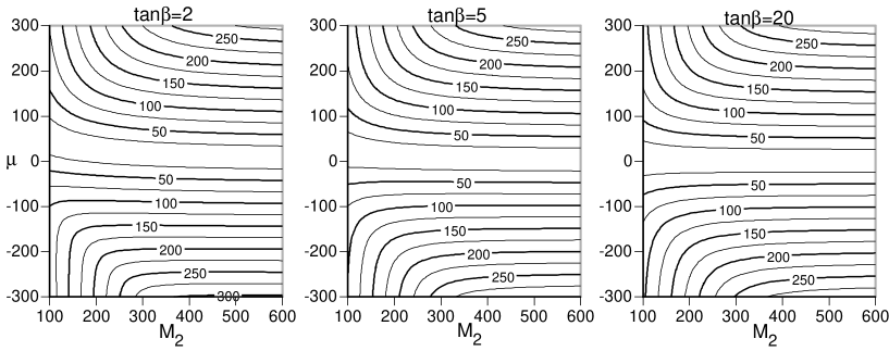
Figure 1: Contour plots of the mass of the lighter chargino as function of the MSSM parameters $M_{2}$ and $\mu$ for $\tan\beta=2$, $5$ and $20$, respectively. All the mass units are GeV.

The limits on the masses of the lighter Higgs scalar and pseudoscalar are now $m_{h}>62.5\mbox{GeV}$ and $m_{A}>62.5\mbox{GeV}$[18], although more stringent bounds are reported $m_{h}\mathrel{\hbox{\raise 0.86108pt\hbox{$>$}\kern-7.5pt\raise-3.87495pt\hbox{$\sim$}}}75\mbox{GeV}$[19]. The results on $m_{h}$ are plotted in Figs. 2 and 3 for $\tan\beta=2$, in Figs. 4 and 5 and in Figs. 6 and 7. We also calculated $m_{h}$ for $\left|\mu\right|=100\mbox{GeV}$ and $200\mbox{GeV}$ and found that $m_{h}$ behaves in the same manner as the case of $\left|\mu\right|=300\mbox{GeV}$ but its value becomes a bit smaller for smaller $\left|\mu\right|$.

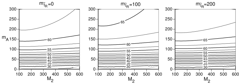
Figure 2: Contour plots of $m_{h}$ as function of the MSSM parameters $M_{2}$ and $m_{A}$ for $\tan\beta=2$, $\mu=-300\mbox{GeV}$ and $m_{{\tilde{t}}_{R}}=0$, $100\mbox{GeV}$ and $200\mbox{GeV}$, respectively. All the mass units are GeV.

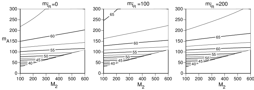
Figure 3: The same as Fig. 2 but for $\tan\beta=2$, $\mu=300\mbox{GeV}$ and $m_{{\tilde{t}}_{R}}=0$, $100\mbox{GeV}$ and $200\mbox{GeV}$, respectively. All the mass units are GeV.

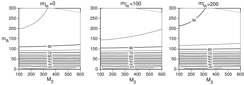
Figure 4: The same as Fig. 2 but for $\tan\beta=5$, $\mu=-300\mbox{GeV}$ and $m_{{\tilde{t}}_{R}}=0$, $100\mbox{GeV}$ and $200\mbox{GeV}$, respectively. All the mass units are GeV.

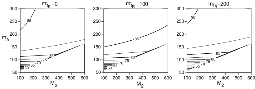
Figure 5: The same as Fig. 2 but for $\tan\beta=5$, $\mu=300\mbox{GeV}$ and $m_{{\tilde{t}}_{R}}=0$, $100\mbox{GeV}$ and $200\mbox{GeV}$, respectively. All the mass units are GeV.

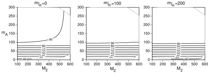
Figure 6: The same as Fig. 2 but for $\tan\beta=20$, $\mu=-300\mbox{GeV}$ and $m_{{\tilde{t}}_{R}}=0$, $100\mbox{GeV}$ and $200\mbox{GeV}$, respectively. All the mass units are GeV.

Figure 7: The same as Fig. 2 but for $\tan\beta=20$, $\mu=300\mbox{GeV}$ and $m_{{\tilde{t}}_{R}}=0$, $100\mbox{GeV}$ and $200\mbox{GeV}$, respectively. All the mass units are GeV.

For $\mu=300\mbox{GeV}$, in the blank region at small $m_{A}$ and large $M_{2}$ region, the point ${\mib v}=(v_{0}\cos\beta,v_{0}\sin\beta)$ is not a local minimum but a saddle point. This region is broader for larger $\tan\beta$, which corresponds to smaller top Yukawa coupling. This is because for larger $M_{2}$, the contributions from the charginos and neutralinos to the effective potential, which are negative, dominate over the bosonic contributions and make the vacuum unstable. For $\tan\beta=2$, the experimental bound on $m_{h}$ is satisfied for $m_{A}\mathrel{\hbox{\raise 0.86108pt\hbox{$>$}\kern-7.5pt\raise-3.87495pt\hbox{$\sim$}}}200-300\mbox{GeV}$, depending on $\mu$ and $M_{2}$. For $\tan\beta\geq 5$, it is satisfied for $m_{A}\mathrel{\hbox{\raise 0.86108pt\hbox{$>$}\kern-7.5pt\raise-3.87495pt\hbox{$\sim$}}}100\mbox{GeV}$.

At finite temperatures, the minimum of the effective potential differs from that at zero temperature. What we concern here are the order of the EWPT and transition temperature $T_{C}$, at which two minima of the effective potential degenerate, and the location of the minimum at $T_{C}$ when it is of first order. These are important ingredients for the electroweak baryogenesis. For definiteness, we take $\mu=-300\mbox{GeV}$, $M_{2}=M_{1}=350\mbox{GeV}$, $m_{{\tilde{t}}_{L}}=400\mbox{GeV}$ and $A_{t}=10\mbox{GeV}$. By use of the numerical method explained in the previous section, we search the minimum of the effective potential at various temperatures to find the transition temperature. This analysis is done for $\tan\beta=2$, $5$ and $20$ with various $m_{{\tilde{t}}_{R}}\geq 0$ and two values of $m_{3}^{2}$ being tuned so that $m_{h}\simeq 62.5\mbox{GeV}$ and $m_{h}\simeq 80\mbox{GeV}$, respectively, for $m_{{\tilde{t}}_{R}}=0$.

For $\tan\beta=2$ and small $m_{{\tilde{t}}_{R}}$, it is difficult to have $m_{h}$ larger than $70\mbox{GeV}$ as seen from Fig. 2. We have adopted $m_{3}^{2}=2.5\times 10^{4}\mbox{GeV}^{2}$, for which $m_{h}\simeq 62.5\mbox{GeV}$ when $m_{{\tilde{t}}_{R}}=0$. Dependences of $v_{C}/T_{C}$, $\tan\beta(T_{C})$ and the masses on $m_{{\tilde{t}}_{R}}$ are plotted in Fig. 8. The condition for the sphaleron decoupling after the EWPT (3.7) is satisfied for $m_{{\tilde{t}}_{R}}\mathrel{\hbox{\raise 0.86108pt\hbox{$<$}\kern-7.5pt\raise-3.87495pt\hbox{$\sim$}}}75\mbox{GeV}$, for which $m_{h}\mathrel{\hbox{\raise 0.86108pt\hbox{$<$}\kern-7.5pt\raise-3.87495pt\hbox{$\sim$}}}64\mbox{GeV}$ and $m_{A}\simeq 239\mbox{GeV}$. The transition temperature varies from $T_{C}=77.3\mbox{GeV}$ ($m_{{\tilde{t}}_{R}}=0$) to $88.7\mbox{GeV}$ ($m_{{\tilde{t}}_{R}}=120\mbox{GeV}$) monotonously. $\tan\beta$ at $T_{C}$ is almost independent of $m_{{\tilde{t}}_{R}}$ and remains to be the zero temperature value.

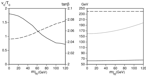
Figure 8: Dependence of $v_{C}/T_{C}$ (solid curve) and $\tan\beta(T_{C})$ (dashed curve) on $m_{{\tilde{t}}_{R}}$ for $m_{3}^{2}=2.5\times 10^{4}\mbox{GeV}^{2}$. $m_{h}$ (solid curve), $m_{A}$ (dashed curve) and $m_{{\tilde{t}}_{1}}$ (dotted curve) are also shown for the same parameter set.

For $\tan\beta=5$, we have taken $m_{3}^{2}=3050\mbox{GeV}^{2}$ and $4624\mbox{GeV}^{2}$, which correspond to $m_{h}\simeq 62.5\mbox{GeV}$ and $80\mbox{GeV}$, respectively. $T_{C}$ is monotonously decreasing with respect to $m_{{\tilde{t}}_{R}}$ and for the former case, $93.2\mbox{GeV}\leq T_{C}\leq 100.5\mbox{GeV}$, while $93.0\mbox{GeV}\leq T_{C}\leq 100.2\mbox{GeV}$ for the latter case. Dependence of $T_{C}$ on $m_{3}^{2}$, so that on $m_{A}$, appears to be weak. $v_{C}/T_{C}$, $\tan\beta(T_{C})$ and the masses are plotted in Fig. 9 and Fig. 10. The condition (3.7) is satisfied for $m_{{\tilde{t}}_{R}}\mathrel{\hbox{\raise 0.86108pt\hbox{$<$}\kern-7.5pt\raise-3.87495pt\hbox{$\sim$}}}50\mbox{GeV}$. $\tan\beta$ at $T_{C}$ receives finite-temperature corrections to become about $20$% larger than the zero-temperature value for the case of the larger $m_{A}$.

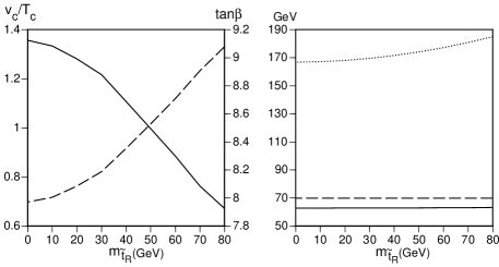
Figure 9: The same as Fig. 8 but for $\tan\beta=5$ and $m_{3}^{2}=3050\mbox{GeV}^{2}$.

Figure 10: The same as Fig. 8 but for $\tan\beta=5$ and $m_{3}^{2}=4624\mbox{GeV}^{2}$.

For $\tan\beta=20$, we adopted $m_{3}^{2}=2308\mbox{GeV}^{2}$ and $2440\mbox{GeV}^{2}$. Dependence of $T_{C}$ on $m_{{\tilde{t}}_{R}}$ and $m_{3}^{2}$ is similar to the previous examples of $\tan\beta=5$. Now $97.2\mbox{GeV}\leq T_{C}\leq 104.5\mbox{GeV}$ for both choices of $m_{3}^{2}$. $v_{C}/T_{C}$, $\tan\beta(T_{C})$ and the masses are plotted in Fig. 11 and Fig. 12. In this case, $\tan\beta(T_{C})$ drastically deviate from the zero-temperature value.

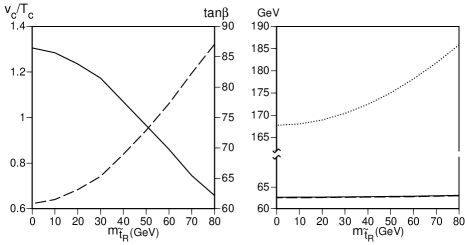
Figure 11: The same as Fig. 8 but for $\tan\beta=20$ and $m_{3}^{2}=2308\mbox{GeV}^{2}$.

Figure 12: The same as Fig. 8 but for $\tan\beta=20$ and $m_{3}^{2}=2440\mbox{GeV}^{2}$.

In order to determine the profile of the bubble wall created at the first-order EWPT, we must know the global structure of the effective potential at $T_{C}$. As an example, we show the contour plot of the effective potential at $T=0$ and $T=T_{C}$ for the case of $\tan\beta=5$, $m_{3}^{2}=4624\mbox{GeV}$ and $m_{{\tilde{t}}_{R}}=0$ in Fig. 13.

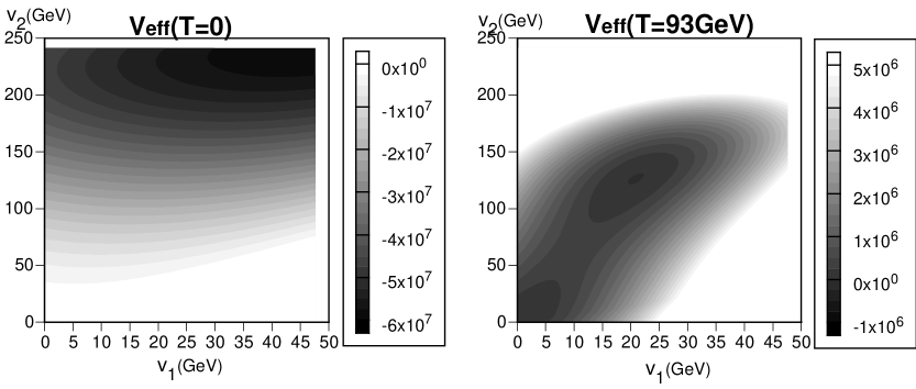
Figure 13: Contour plots of the effective potential at $T=0$ and $T=T_{C}$ for $\tan\beta=5$, $m_{3}^{2}=4624\mbox{GeV}^{2}$ and $m_{{\tilde{t}}_{R}}=0$.

This shows that two degenerate minima at $T_{C}$ is connected by a valley with almost constant $\tan\beta(T_{C})\simeq 6$. This is also the case for the other sets of the parameters we studied. Some of the baryogenesis scenarios based on the MSSM requires that $\tan\beta$ varies spatially around the bubble wall. But this result implies that $\tan\beta$ remains to be almost constant around the wall.

4.2 $\mib{CP}$-violating case

In the MSSM, there are many sources of $CP$ violation other than the phase in the CKM matrix. Among them are relative phases of the complex parameters $\mu$, $A_{t}$, $M_{2}$ and $M_{1}$. These also induce $CP$ violation in the Higgs sector, which is the relative phase $\theta$ of the VEVs of the two Higgs doublets. This $\theta$ together with the other $CP$-violating phases affect such observables as the electric dipole moment of the neutron. Hence knowledge of $\theta$ is necessary to find bounds on the phases of the complex parameters in the MSSM. $\theta={\rm Arg}(v_{2}+iv_{3})$ in the gauge with $v_{4}=0$ is determined by minimizing the effective potential at $T=0$. Even when all the parameters are real, the effective potential could have $CP$-violating vacuum. This is know as the spontaneous $CP$ violation, but in the MSSM it inevitably accompanies a too light scalar[20]. We found that this is the case. Indeed if we take $\tan\beta=5$ and $m_{{\tilde{t}}_{R}}=0$ and tune $m_{3}^{2}=2113.3\mbox{GeV}^{2}$, the effective potential has two degenerate minima which correspond to $\theta=\pm 0.318$ and $\tan\beta=4.917$. Then the lightest scalar mass is $12.9\mbox{GeV}$, which differs from any mass from the mass formulas because of large mixing of the $CP$ eigenstates.

Now we study the effect of explicit $CP$ violation in the complex parameters on the $CP$ violation in the Higgs sector. As the first example, we take $\tan\beta=5$, $m_{{\tilde{t}}_{R}}=0$, $m_{3}^{2}=4624\mbox{GeV}^{2}$, $\mu=-300\cdot e^{i\delta_{\mu}}$ and the remaining parameters are set to be the values adopted in the previous subsection. For nonzero $\delta_{\mu}$, $\theta$ have nonzero value and the scalar and pseudoscalar mixes to form the mass eigenstates. By the numerical method, the minimum of the effective potential were searched and the second derivatives at the minimum was evaluated to calculate the masses of the Higgs bosons, for $0\leq\delta_{\mu}\leq 0.1$. Dependence of $\theta$, $\tan\beta$ and masses of two light bosons on $\delta_{\mu}$ is depicted in Fig. 14.

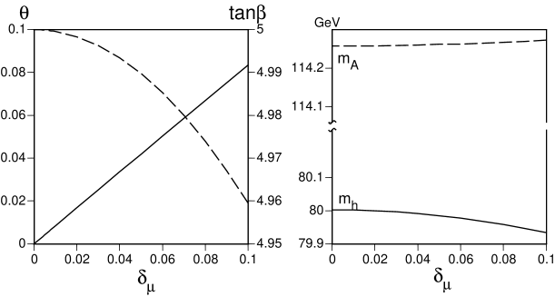
Figure 14: Dependence of $\theta$ (solid curve), $\tan\beta$ (dashed curve) and Higgs masses on $\delta_{\mu}$.

Within this range of $\delta_{\mu}$, the derivation of the masses from the values at $\delta_{\mu}$ is negligible. The induced $\theta$ is the same order and has the same sign as $\delta_{\mu}$. By linearly fitting, we find $\theta=0.8265\cdot\delta_{\mu}$. By redefining the fields, we find that the physical $CP$-violating phase in the mass matrices (2.15), (2.16) and (2.17) is $\delta_{\mu}+\theta$. Hence $\delta_{\mu}$ enhances the magnitude of $CP$ violation.

As a second example, we put $M_{2}=M_{1}=350\cdot e^{i\delta_{2}}\mbox{GeV}$ and all the rest parameters are taken to be real and set to the same values as the previous example. Dependence of $\theta$, $\tan\beta$ and masses of two light bosons on $\delta_{\mu}$ is shown in Fig. 15.

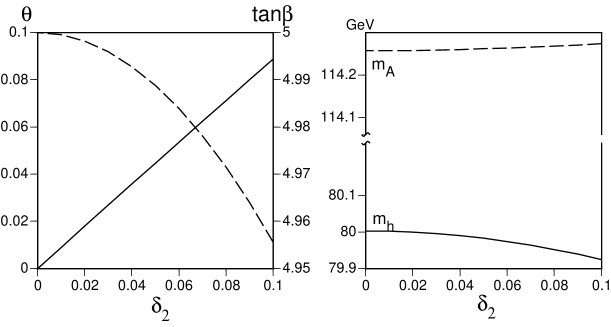
Figure 15: Dependence of $\theta$ (solid curve), $\tan\beta$ (dashed curve) and Higgs masses on $\delta_{2}$.

The induced $CP$ phase is fitted to $\theta=0.8885\cdot\delta_{2}$, which has the same sign as the original $\delta_{2}$. Since the physical $CP$ phase in the mass matrix (2.16) is $\delta_{2}+\theta$, the $CP$-violating phase is enhanced by the radiative corrections.

In the scenario of the electroweak baryogenesis, the $CP$ violation around the bubble wall is a key ingredient and it is determined by solving the equations of motion with the effective potential at $T_{C}$. Then the VEVs in the two degenerate minima provide the boundary conditions to these equations. Although spontaneous $CP$ violation at $T\simeq T_{C}$ could occur, it would accompany a too light scalar at zero temperature. Any way, an explicit $CP$ violation is necessary to resolve degeneracy in energy of the $CP$-conjugate pair of the bubble walls, otherwise no net baryon asymmetry would survive the EWPT. For the same parameters as the zero temperature case, we plot in Fig. 16 dependences of the induced $CP$ violating phase $\theta$ and $\tan\beta$ on the phase of the $\mu$-parameter.

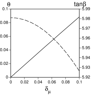
Figure 16: Dependence of $\theta$ (solid curve), $\tan\beta$ (dashed curve) at $T=92\mbox{GeV}$.

The behaviors of $\theta$ and $\tan\beta$ are almost the same as those at zero temperature, but $\theta=0.8862\cdot\delta_{\mu}$.

5 Discussion

We have studied the masses of the neutral Higgs bosons and the electroweak phase transition of the MSSM by use of the one-loop effective potential. For the parameters we adopted, the contributions from the charginos and neutralinos are shown not to be negligible. We have found that the EWPT is of so strongly first order that the sphaleron process after it decouples, for $m_{{\tilde{t}}_{R}}\mathrel{\hbox{\raise 0.86108pt\hbox{$<$}\kern-7.5pt\raise-3.87495pt\hbox{$\sim$}}}75\mbox{GeV}$ when $\tan\beta=2$, $m_{h}=62.8\mbox{GeV}$ and $m_{A}=239\mbox{GeV}$, for $m_{{\tilde{t}}_{R}}\mathrel{\hbox{\raise 0.86108pt\hbox{$<$}\kern-7.5pt\raise-3.87495pt\hbox{$\sim$}}}50\mbox{GeV}$ when $\tan\beta=5$, $m_{h}=62.8\mbox{GeV}$ and $m_{A}=70\mbox{GeV}$, for $m_{{\tilde{t}}_{R}}\mathrel{\hbox{\raise 0.86108pt\hbox{$<$}\kern-7.5pt\raise-3.87495pt\hbox{$\sim$}}}53\mbox{GeV}$ when $\tan\beta=5$, $m_{h}=80\mbox{GeV}$ and $m_{A}=114\mbox{GeV}$, for $m_{{\tilde{t}}_{R}}\mathrel{\hbox{\raise 0.86108pt\hbox{$<$}\kern-7.5pt\raise-3.87495pt\hbox{$\sim$}}}46.7\mbox{GeV}$ when $\tan\beta=20$, $m_{h}=62.7\mbox{GeV}$ and $m_{A}=62.6\mbox{GeV}$, and for $m_{{\tilde{t}}_{R}}\mathrel{\hbox{\raise 0.86108pt\hbox{$<$}\kern-7.5pt\raise-3.87495pt\hbox{$\sim$}}}46.8\mbox{GeV}$ when $\tan\beta=20$, $m_{h}=80\mbox{GeV}$ and $m_{A}=81\mbox{GeV}$. These bounds on $m_{{\tilde{t}}_{R}}$ almost correspond to a bound on the lighter stop mass $m_{{\tilde{t}}_{1}}\leq m_{t}$. For the parameters which permit strongly first-order EWPT, we have investigated $\tan\beta$ at the transition temperature. It receives larger temperature-corrections for larger $\tan\beta$ at zero temperature, which corresponds to smaller Yukawa coupling of the top quark. This suggests importance of finite-temperature contributions from the particles other than the top quark and squarks. We also studied $CP$ violation in the Higgs sector, which is characterized by the relative phase $\theta$ of the expectation values of the two Higgs doublets. As is well known, the spontaneous mechanism to generate $\theta$ accompanies a too light scalar. An explicit $CP$ violation in the complex parameters induces $\theta$ of the same order and sign as itself, through radiative and finite-temperature corrections. This implies that the physical phases in the mass matrices of the chargino, neutralino and stop are enhanced by the complex phases which are originally contained in these matrices. Hence one must take this effect into account to find bounds on the parameters in the MSSM obtained from such data as the neutron EDM.

Some of the mechanism of electroweak baryogenesis in the MSSM requires $\tan\beta$ to vary spatially. But at the transition temperature, it stays almost constant at $\tan\beta(T_{C})$. Then viable scenarios of the electroweak baryogenesis rely on spatially varying $\theta$ and/or $\left|\mib v\right|$ in the presence explicit $CP$ violation. The spatial dependence of $\theta$ and $\left|\mib v\right|$ around the bubble wall created at the EWPT is examined in [15]. The values of these variables in the broken phase at $T_{C}$ obtained here will serve as the boundary conditions to the dynamical equations for $(\theta(x),\left|{\mib v}(x)\right|)$. These functions in the MSSM will be studied elsewhere[21].

In this paper, we extensively used the one-loop effective potential for self-containedness. Extension to the two-loop resummed potential would be straightforward. The two-loop resummed potential without the contributions from the charginos and neutralinos yields strongly first-order EWPT for a wider range of parameters than the corresponding one-loop potential[11]. We expect that if the higher-order effects are taken into account, the effective potential including the contributions from all the particles in the MSSM will provide strongly first-order EWPT for a broader region in the parameter space than that investigated here.

Appendix A Derivatives of the Effective Potential

We present the formulas for the first and second derivatives of the effective potential evaluated at a $CP$-conserving vacuum. Since all the parameters are assumed to be real, $CP$ is conserved so that $v_{3}=v_{4}=0$ at the vacuum. But we retain $v_{3}$ to derive the mass of the $CP$-odd scalar according to (2.20). To see contribution from each species, we give the derivatives of the correction to the effective potential from each particle.

A.1 gauge bosons

The contributions to the effective potential is given by (2.8). Its first derivatives at the vacuum are

$${1\over{v_{1}}}{{\partial\Delta_{g}V({\mib v})}\over{\partial v_{1}}} = {1\over{v_{2}}}{{\partial\Delta_{g}V({\mib v})}\over{\partial v_{2}}}$$

$$= 6\cdot{{g_{2}^{2}}\over 2}{{m_{W}^{2}({\mib v})}\over{32\pi^{2}}}\left(\log{{m_{W}^{2}({\mib v})}\over{M_{\rm ren}^{2}}}-1\right)+3\cdot{{g_{2}^{2}+g_{1}^{2}}\over 2}{{m_{Z}^{2}({\mib v})}\over{32\pi^{2}}}\left(\log{{m_{Z}^{2}({\mib v})}\over{M_{\rm ren}^{2}}}-1\right).$$

It is straightforward to calculate the second derivatives:

$$v_{1}{\partial\over{\partial v_{1}}}\left({1\over{v_{1}}}{{\partial\Delta_{g}V({\mib v})}\over{\partial v_{1}}}\right) = {{3\cos^{2}\beta}\over{8\pi^{2}v_{0}^{2}}}\left[2m_{W}^{4}\log{{m_{W}^{2}({\mib v})}\over{M_{\rm ren}^{2}}}+m_{Z}^{4}\log{{m_{Z}^{2}({\mib v})}\over{M_{\rm ren}^{2}}}\right],$$ (A.2)

$$v_{2}{\partial\over{\partial v_{2}}}\left({1\over{v_{2}}}{{\partial\Delta_{g}V({\mib v})}\over{\partial v_{2}}}\right) = {{3\sin^{2}\beta}\over{8\pi^{2}v_{0}^{2}}}\left[2m_{W}^{4}\log{{m_{W}^{2}({\mib v})}\over{M_{\rm ren}^{2}}}+m_{Z}^{4}\log{{m_{Z}^{2}({\mib v})}\over{M_{\rm ren}^{2}}}\right],$$ (A.3)

$${{\partial^{2}\Delta_{g}V({\mib v})}\over{\partial v_{1}\partial v_{2}}} = {{3\sin\beta\cos\beta}\over{8\pi^{2}v_{0}^{2}}}\left[2m_{W}^{4}\log{{m_{W}^{2}({\mib v})}\over{M_{\rm ren}^{2}}}+m_{Z}^{4}\log{{m_{Z}^{2}({\mib v})}\over{M_{\rm ren}^{2}}}\right],$$

$${{\partial^{2}\Delta_{g}V({\mib v})}\over{\partial v_{3}^{2}}} = {1\over{v_{3}}}{{\partial\Delta_{g}V({\mib v})}\over{\partial v_{3}}}={1\over{v_{2}}}{{\partial\Delta_{g}V({\mib v})}\over{\partial v_{2}}}.$$ (A.5)

A.2 top quark

Since the contribution from the top quark (2.9) is independent of $v_{1}$, any derivative with respect to $v_{1}$ vanishes.

$${1\over{v_{1}}}{{\partial\Delta_{g}V({\mib v})}\over{\partial v_{1}}} = 0,$$

$${1\over{v_{2}}}{{\partial\Delta_{g}V({\mib v})}\over{\partial v_{2}}} = {1\over{v_{3}}}{{\partial\Delta_{g}V({\mib v})}\over{\partial v_{3}}}=-12\cdot y_{t}^{2}{{m_{t}^{2}({\mib v})}\over{32\pi^{2}}}\left(\log{{m_{t}^{2}({\mib v})}\over{M_{\rm ren}^{2}}}-1\right),$$ (A.6)

and

$$v_{1}{\partial\over{\partial v_{1}}}\left({1\over{v_{1}}}{{\partial\Delta_{t}V({\mib v})}\over{\partial v_{1}}}\right) = {{\partial^{2}\Delta_{t}V({\mib v})}\over{\partial v_{1}\partial v_{2}}}=0,$$ (A.7)

$$v_{2}{\partial\over{\partial v_{2}}}\left({1\over{v_{2}}}{{\partial\Delta_{t}V({\mib v})}\over{\partial v_{2}}}\right) = -12\cdot{{4m_{t}^{4}({\mib v})}\over{v_{0}^{2}\sin^{2}\beta}}{1\over{32\pi^{2}}}\log{{m_{t}^{2}({\mib v})}\over{M_{\rm ren}^{2}}},$$ (A.8)

$${{\partial^{2}\Delta_{t}V({\mib v})}\over{\partial v_{3}^{2}}} = {1\over{v_{2}}}{{\partial\Delta_{t}V({\mib v})}\over{\partial v_{2}}}.$$ (A.9)

A.3 top squarks

The stop contribution is given by (2.10), in which the mass eigenvalues are

$$m_{{\tilde{t}}_{a}}^{2}({\mib v}) = {{m_{{\tilde{t}}_{L}}^{2}+m_{{\tilde{t}}_{R}}^{2}}\over 2}+{{g_{2}^{2}+g_{1}^{2}}\over 8}(v_{1}^{2}-v_{2}^{2}-v_{3}^{2})+m_{t}^{2}({\mib v})$$

$$\pm\sqrt{\left({{m_{{\tilde{t}}_{L}}^{2}-m_{{\tilde{t}}_{R}}^{2}}\over 2}+{{3g_{2}^{2}-5g_{1}^{2}}\over{24}}(v_{1}^{2}-v_{2}^{2}-v_{3}^{2})\right)^{2}+{{y_{t}^{2}}\over 2}\left[(\mu v_{1}+A_{t}v_{2})^{2}+A_{t}^{2}v_{3}^{2}\right]}.$$

The first derivatives are given by

$${1\over{v_{i}}}{{\partial\Delta_{\tilde{t}}V({\mib v})}\over{\partial v_{i}}}=6\sum_{a=1,2}{1\over{v_{i}}}{{\partial m_{{\tilde{t}}_{a}}^{2}({\mib v})}\over{\partial v_{i}}}{{m_{{\tilde{t}}_{a}}^{2}({\mib v})}\over{32\pi^{2}}}\left(\log{{m_{{\tilde{t}}_{a}}^{2}({\mib v})}\over{M_{\rm ren}^{2}}}-1\right),$$ (A.11)

where the first derivatives of the stop mass-squared evaluated at the vacuum are

$${1\over{v_{1}}}{{\partial m_{{\tilde{t}}_{a}}^{2}}\over{\partial v_{1}}} = {{2m_{t}^{2}}\over{v_{0}^{2}\sin^{2}\beta}}\left({{m_{Z}^{2}\sin^{2}\beta}\over{2m_{t}^{2}}}\pm{{n_{\tilde{t}}^{(1)}}\over{R_{\tilde{t}}}}\right),$$ (A.12)

$${1\over{v_{2}}}{{\partial m_{{\tilde{t}}_{a}}^{2}}\over{\partial v_{2}}} = {{2m_{t}^{2}}\over{v_{0}^{2}\sin^{2}\beta}}\left(1-{{m_{Z}^{2}\sin^{2}\beta}\over{2m_{t}^{2}}}\pm{{n_{\tilde{t}}^{(2)}}\over{R_{\tilde{t}}}}\right),$$ (A.13)

$${1\over{v_{3}}}{{\partial m_{{\tilde{t}}_{a}}^{2}}\over{\partial v_{3}}} = {{2m_{t}^{2}}\over{v_{0}^{2}\sin^{2}\beta}}\left(1-{{m_{Z}^{2}\sin^{2}\beta}\over{2m_{t}^{2}}}\pm{{-{{8m_{W}^{2}-5m_{Z}^{2}}\over{6m_{t}^{2}}}d_{\tilde{t}}\sin^{2}\beta+{1\over 2}A_{t}^{2}}\over{R_{\tilde{t}}}}\right),$$ (A.14)

with

$$d_{\tilde{t}} = {{m_{{\tilde{t}}_{L}}^{2}-m_{{\tilde{t}}_{R}}^{2}}\over 2}+{{8m_{W}^{2}-5m_{Z}^{2}}\over 6}\cos(2\beta),$$

$$n_{\tilde{t}}^{(1)} = {{8m_{W}^{2}-5m_{Z}^{2}}\over{6m_{t}^{2}}}d_{\tilde{t}}\sin^{2}\beta+{1\over 2}\mu(\mu+A_{t}\tan\beta),$$

$$n_{\tilde{t}}^{(2)} = -{{8m_{W}^{2}-5m_{Z}^{2}}\over{6m_{t}^{2}}}d_{\tilde{t}}\sin^{2}\beta+{1\over 2}A_{t}(\mu\cot\beta+A_{t}),$$

$$R_{\tilde{t}} = \sqrt{d_{\tilde{t}}^{2}+m_{t}^{2}(\mu\cot\beta+A_{t})^{2}}.$$ (A.15)

The general expression for the second derivatives is given by

$$v_{j}{\partial\over{\partial v_{i}}}\left({1\over{v_{j}}}{{\partial\Delta_{\tilde{t}}V({\mib v})}\over{\partial v_{j}}}\right) = 6\sum_{a=1,2}\Biggl{[}v_{j}{\partial\over{\partial v_{i}}}\left({1\over{v_{j}}}{{\partial m_{{\tilde{t}}_{a}}^{2}({\mib v})}\over{\partial v_{j}}}\right){{m_{{\tilde{t}}_{a}}^{2}({\mib v})}\over{32\pi^{2}}}\left(\log{{m_{{\tilde{t}}_{a}}^{2}({\mib v})}\over{M_{\rm ren}^{2}}}-1\right)$$ (A.16)

$$\qquad\qquad\qquad+{{\partial m_{{\tilde{t}}_{a}}^{2}({\mib v})}\over{\partial v_{i}}}{{\partial m_{{\tilde{t}}_{a}}^{2}({\mib v})}\over{\partial v_{j}}}{1\over{32\pi^{2}}}\log{{m_{{\tilde{t}}_{a}}^{2}({\mib v})}\over{M_{\rm ren}^{2}}}\Biggr{]}$$

The relevant second derivatives to this expression are

$$v_{1}{\partial\over{\partial v_{1}}}\left({1\over{v_{1}}}{{\partial m_{{\tilde{t}}_{a}}^{2}}\over{\partial v_{1}}}\right) = \pm{{\cos^{2}\beta}\over{v_{0}^{2}}}\left[{{\left({{8m_{W}^{2}-5m_{Z}^{2}}\over 3}\right)^{2}-{{\mu A_{t}m_{t}^{2}}\over{\sin\beta\cos^{3}\beta}}}\over{R_{\tilde{t}}}}-{{\left(n_{\tilde{t}}^{(1)}\right)^{2}}\over{R_{\tilde{t}}^{3}}}\right],$$ (A.17)

$$v_{2}{\partial\over{\partial v_{2}}}\left({1\over{v_{2}}}{{\partial m_{{\tilde{t}}_{a}}^{2}}\over{\partial v_{2}}}\right) = \pm{{\sin^{2}\beta}\over{v_{0}^{2}}}\left[{{\left({{8m_{W}^{2}-5m_{Z}^{2}}\over 3}\right)^{2}-{{\mu A_{t}m_{t}^{2}\cos\beta}\over{\sin^{5}\beta}}}\over{R_{\tilde{t}}}}-{{\left(n_{\tilde{t}}^{(2)}\right)^{2}}\over{R_{\tilde{t}}^{3}}}\right],$$ (A.18)

$${{\partial^{2}m_{{\tilde{t}}_{a}}^{2}}\over{\partial v_{1}\partial v_{2}}} = \pm{{\sin\beta\cos\beta}\over{v_{0}^{2}}}\left[{{-\left({{8m_{W}^{2}-5m_{Z}^{2}}\over 3}\right)^{2}+{{\mu A_{t}m_{t}^{2}}\over{\sin^{3}\beta\cos\beta}}}\over{R_{\tilde{t}}}}-{{n_{\tilde{t}}^{(1)}n_{\tilde{t}}^{(2)}}\over{R_{\tilde{t}}^{3}}}\right],$$ (A.19)

$$v_{3}{\partial\over{\partial v_{3}}}\left({1\over{v_{3}}}{{\partial m_{{\tilde{t}}_{a}}^{3}}\over{\partial v_{3}}}\right) = 0.$$ (A.20)

A.4 charginos

The derivatives of (2.11) are evaluated in the same manner as the case of the stop. The mass-squared eigenvalues are

$$m_{\chi^{\pm}_{a}}^{2}({\mib v}) = m_{W}^{2}({\mib v})+{{M_{2}^{2}+\mu^{2}}\over 2}$$

$$\pm\sqrt{\left({{M_{2}^{2}-\mu^{2}}\over 2}+{{g_{2}^{2}}\over 4}(v_{1}^{2}-v_{2}^{2}-v_{3}^{2})\right)^{2}+{{g_{2}^{2}}\over 2}\left[(\mu v_{1}+M_{2}v_{2})^{2}+M_{2}^{2}v_{3}^{2}\right]}.$$

The first derivatives of the corrections to the effective potential is given by a similar expression to (A.11), in which the relevant derivatives of the masses-squared are

$${1\over{v_{1}}}{{\partial m_{\chi^{\pm}_{a}}^{2}}\over{\partial v_{1}}} = {{2m_{W}^{2}}\over{v_{0}^{2}}}\left(1\pm{{n_{\chi}^{(1)}}\over{R_{\chi}}}\right),$$ (A.22)

$${1\over{v_{2}}}{{\partial m_{\chi^{\pm}_{a}}^{2}}\over{\partial v_{2}}} = {{2m_{W}^{2}}\over{v_{0}^{2}}}\left(1\pm{{n_{\chi}^{(2)}}\over{R_{\chi}}}\right),$$ (A.23)

$${1\over{v_{3}}}{{\partial m_{\chi^{\pm}_{a}}^{2}}\over{\partial v_{3}}} = {{2m_{W}^{2}}\over{v_{0}^{2}}}\left(1\pm{{{{M_{2}^{2}+\mu^{2}}\over 2}-m_{W}^{2}\cos(2\beta)}\over{R_{\chi}}}\right),$$ (A.24)

where

$$n_{\chi}^{(1)} = {{M_{2}^{2}+\mu^{2}}\over 2}+m_{W}^{2}\cos(2\beta)+\mu M_{2}\tan\beta,$$

$$n_{\chi}^{(2)} = {{M_{2}^{2}+\mu^{2}}\over 2}-m_{W}^{2}\cos(2\beta)+\mu M_{2}\cot\beta,$$

$$R_{\chi} = \sqrt{\left({{M_{2}^{2}-\mu^{2}}\over 2}+m_{W}^{2}\cos(2\beta)\right)^{2}+2m_{W}^{2}(M_{2}\sin\beta+\mu\cos\beta)^{2}}.$$ (A.25)

The second derivatives have the same form as (A.16) except for the overall coefficient. The relevant second derivatives are given by

$$v_{1}{\partial\over{\partial v_{1}}}\left({1\over{v_{1}}}{{\partial m_{\chi^{\pm}_{a}}^{2}}\over{\partial v_{1}}}\right) = \pm{{2m_{W}^{2}}\over{v_{0}^{2}}}\left[{{2m_{W}^{2}\cos^{2}\beta-\mu M_{2}\tan\beta}\over{R_{\chi}}}-{{2m_{W}^{2}\left(n_{\chi}^{(1)}\right)^{2}\cos^{2}\beta}\over{R_{\chi}^{3}}}\right],$$

$$v_{2}{\partial\over{\partial v_{2}}}\left({1\over{v_{2}}}{{\partial m_{\chi^{\pm}_{a}}^{2}}\over{\partial v_{2}}}\right) = \pm{{2m_{W}^{2}}\over{v_{0}^{2}}}\left[{{2m_{W}^{2}\sin^{2}\beta-\mu M_{2}\cot\beta}\over{R_{\chi}}}-{{2m_{W}^{2}\left(n_{\chi}^{(1)}\right)^{2}\sin^{2}\beta}\over{R_{\chi}^{3}}}\right],$$

$${{\partial^{2}m_{\chi^{\pm}_{a}}^{2}}\over{\partial v_{1}\partial v_{2}}} = \pm{{2m_{W}^{2}}\over{v_{0}^{2}}}\left[{{-2m_{W}^{2}\sin\beta\cos\beta+\mu M_{2}}\over{R_{\chi}}}-{{2m_{W}^{2}n_{\chi}^{(1)}n_{\chi}^{(2)}\sin\beta\cos\beta}\over{R_{\chi}^{3}}}\right],$$

$$v_{3}{\partial\over{\partial v_{3}}}\left({1\over{v_{3}}}{{\partial m_{\chi^{\pm}_{a}}^{2}}\over{\partial v_{3}}}\right) = 0.$$ (A.29)

A.5 neutralinos

Although the neutralino contribution to the effective potential is given by (2.12) in terms of the mass eigenvalues, it is difficult to work out its derivatives, since the eigenvalues have complicated forms. To avoid this complexity, we return to the original form of the neutralino contribution:

$$\Delta_{\chi^{0}}V({\mib v})={i\over 2}\int_{k}{\rm Tr}\,\log\left[D_{\chi^{0}}^{-1}(k;{\mib v})\right],$$ (A.30)

where $\int_{k}$ denotes the integral over the Minkowskian momentum, the trace is taken over the index of 4-dimensional internal space and the spinor index, and $D_{\chi^{0}}$ is the four-component Dirac operator defined by

$$D_{\chi^{0}}^{-1}(k;{\mib v})=k\kern-5.0pt\raise 0.60277pt\hbox{/}-M_{\chi^{0}}{{1-\gamma_{5}}\over 2}-M_{\chi^{0}}^{\dagger}{{1+\gamma_{5}}\over 2}.$$ (A.31)

Here the mass matrix $M_{\chi^{0}}$ is defined by (2.17). The first and second derivatives of (A.30) have the forms of

$${{\partial\Delta_{\chi^{0}}V({\mib v})}\over{\partial v_{i}}} = {i\over 2}\int_{k}{\rm Tr}\left[D_{\chi^{0}}(k;{\mib v}){{\partial D_{\chi^{0}}^{-1}(k;{\mib v})}\over{\partial v_{i}}}\right],$$

$${{\partial^{2}\Delta_{\chi^{0}}V({\mib v})}\over{\partial v_{i}\partial v_{j}}} = -{i\over 2}\int_{k}{\rm Tr}\left[D_{\chi^{0}}(k;{\mib v}){{\partial D_{\chi^{0}}^{-1}(k;{\mib v})}\over{\partial v_{i}}}D_{\chi^{0}}(k;{\mib v}){{\partial D_{\chi^{0}}^{-1}(k;{\mib v})}\over{\partial v_{j}}}\right].$$ (A.32)

The integrand of the first derivative evaluated at the vacuum have the following compact form:

$${1\over{v_{i}}}{\rm Tr}\left[D_{\chi^{0}}(k;{\mib v}){{\partial D_{\chi^{0}}^{-1}(k;{\mib v})}\over{\partial v_{i}}}\right]=-{{2m_{Z}^{2}}\over{v_{0}^{2}}}{\rm Tr}\left[{{k\kern-5.0pt\raise 0.60277pt\hbox{/}+\mu_{i}}\over{k^{2}-\mu^{2}}}{{D_{1}(k)}\over{1-m_{Z}^{2}D_{1}(k)D_{2}(k)}}\right],$$ (A.33)

where

$$D_{1}(k)={{\cos^{2}\theta_{W}}\over{k\kern-5.0pt\raise 0.60277pt\hbox{/}-M_{2}}}+{{\sin^{2}\theta_{W}}\over{k\kern-5.0pt\raise 0.60277pt\hbox{/}-M_{1}}},\qquad D_{2}(k)={{k\kern-5.0pt\raise 0.60277pt\hbox{/}+\mu\sin(2\beta)}\over{k^{2}-\mu^{2}}},$$ (A.34)

and

$$\mu_{1}\equiv\mu\tan\beta,\qquad\mu_{2}\equiv\mu\cot\beta.$$ (A.35)

The integrands of the second derivatives are reduced to

$${\rm Tr}\left[D_{\chi^{0}}(k;{\mib v}){{\partial D_{\chi^{0}}^{-1}(k;{\mib v})}\over{\partial v_{1}}}D_{\chi^{0}}(k;{\mib v}){{\partial D_{\chi^{0}}^{-1}(k;{\mib v})}\over{\partial v_{1}}}\right]$$

$$= {{2m_{Z}^{2}}\over{v_{0}^{2}}}{\rm Tr}\left[{k\kern-5.0pt\raise 0.60277pt\hbox{/}\over{k^{2}-\mu^{2}}}{{D_{1}(k)}\over{1-m_{Z}^{2}D_{1}(k)D_{2}(k)}}\right]$$

$$\qquad\qquad+{{4m_{Z}^{4}\cos^{2}\beta}\over{v_{0}^{2}}}{\rm Tr}\left[\left({{k\kern-5.0pt\raise 0.60277pt\hbox{/}+\mu\tan\beta}\over{k^{2}-\mu^{2}}}{{D_{1}(k)}\over{1-m_{Z}^{2}D_{1}(k)D_{2}(k)}}\right)^{2}\right],$$

$${\rm Tr}\left[D_{\chi^{0}}(k;{\mib v}){{\partial D_{\chi^{0}}^{-1}(k;{\mib v})}\over{\partial v_{2}}}D_{\chi^{0}}(k;{\mib v}){{\partial D_{\chi^{0}}^{-1}(k;{\mib v})}\over{\partial v_{2}}}\right]$$

$$= {{2m_{Z}^{2}}\over{v_{0}^{2}}}{\rm Tr}\left[{k\kern-5.0pt\raise 0.60277pt\hbox{/}\over{k^{2}-\mu^{2}}}{{D_{1}(k)}\over{1-m_{Z}^{2}D_{1}(k)D_{2}(k)}}\right]$$

$$\qquad\qquad+{{4m_{Z}^{4}\sin^{2}\beta}\over{v_{0}^{2}}}{\rm Tr}\left[\left({{k\kern-5.0pt\raise 0.60277pt\hbox{/}+\mu\cot\beta}\over{k^{2}-\mu^{2}}}{{D_{1}(k)}\over{1-m_{Z}^{2}D_{1}(k)D_{2}(k)}}\right)^{2}\right],$$

$${\rm Tr}\left[D_{\chi^{0}}(k;{\mib v}){{\partial D_{\chi^{0}}^{-1}(k;{\mib v})}\over{\partial v_{1}}}D_{\chi^{0}}(k;{\mib v}){{\partial D_{\chi^{0}}^{-1}(k;{\mib v})}\over{\partial v_{2}}}\right]$$

$$= {{2m_{Z}^{2}}\over{v_{0}^{2}}}{\rm Tr}\left[{\mu\over{k^{2}-\mu^{2}}}{{D_{1}(k)}\over{1-m_{Z}^{2}D_{1}(k)D_{2}(k)}}\right]$$

$$+ {{4m_{Z}^{4}\sin\beta\cos\beta}\over{v_{0}^{2}}}{\rm Tr}\left[{{k\kern-5.0pt\raise 0.60277pt\hbox{/}+\mu\tan\beta}\over{k^{2}-\mu^{2}}}{{k\kern-5.0pt\raise 0.60277pt\hbox{/}+\mu\cot\beta}\over{k^{2}-\mu^{2}}}\left({{D_{1}(k)}\over{1-m_{Z}^{2}D_{1}(k)D_{2}(k)}}\right)^{2}\right],$$

$${\rm Tr}\left[D_{\chi^{0}}(k;{\mib v}){{\partial D_{\chi^{0}}^{-1}(k;{\mib v})}\over{\partial v_{3}}}D_{\chi^{0}}(k;{\mib v}){{\partial D_{\chi^{0}}^{-1}(k;{\mib v})}\over{\partial v_{3}}}\right]$$

$$= {{2m_{Z}^{2}}\over{v_{0}^{2}}}{\rm Tr}\left[{k\kern-5.0pt\raise 0.60277pt\hbox{/}\over{k^{2}-\mu^{2}}}{{D_{1}(k)}\over{1-m_{Z}^{2}D_{1}(k)D_{2}(k)}}\right]$$

$$- {{4m_{Z}^{4}\cos^{2}\beta}\over{v_{0}^{2}}}{{\mu^{2}}\over{(k^{2}-\mu^{2})^{2}}}{\rm Tr}\left[{{D_{1}(k)}\over{1-m_{Z}^{2}D_{1}(k)D_{2}(k)}}{{D_{1}(-k)}\over{1-m_{Z}^{2}D_{1}(-k)D_{2}(-k)}}\right].$$ (A.39)

For the special case of $M_{2}=M_{1}$ which is extensively investigated in this paper, we have the following formulas for the relevant derivatives to the masses of the neutral Higgs bosons.

$${1\over{v_{i}}}{{\partial\Delta_{\chi^{0}}V({\mib v})}\over{\partial v_{i}}}$$ (A.44)

$$= {{m_{Z}^{2}}\over{4\pi^{2}v_{0}^{2}}}\Biggl{\{}-(\mu^{2}+m_{Z}^{2})\left(\log{{\mu^{2}+m_{Z}^{2}}\over{M_{\rm ren}^{2}}}-1\right)+M_{2}(M_{2}+\mu_{i})L(M_{2}^{2},\mu^{2}+m_{Z}^{2})$$

$$\qquad+\left(1+{{\mu\sin(2\beta)}\over{M_{2}}}\right)m_{Z}^{2}\left[-\left(2+{{\mu_{i}}\over{M_{2}}}\right)F_{1}\left({\mu\over{M_{2}}},{{m_{Z}}\over{M_{2}}},\tan\beta\right)\right.$$

$$\qquad\qquad\qquad\qquad\qquad\qquad\left.+2\left(1+{{\mu_{i}}\over{M_{2}}}\right)F_{2}\left({\mu\over{M_{2}}},{{m_{Z}}\over{M_{2}}},\tan\beta\right)\right]$$

$$\qquad+\left(1+{{\mu\sin(2\beta)}\over{M_{2}}}\right)^{2}{{m_{Z}^{4}}\over{M_{2}^{2}}}\left[F_{3}\left({\mu\over{M_{2}}},{{m_{Z}}\over{M_{2}}},\tan\beta\right)-\left(1+{{\mu_{i}}\over{M_{2}}}\right)F_{4}\left({\mu\over{M_{2}}},{{m_{Z}}\over{M_{2}}},\tan\beta\right)\right\},$$

$$-{1\over{v_{1}}}{{\partial\Delta_{\chi^{0}}V({\mib v})}\over{\partial v_{1}}}+{{\partial^{2}\Delta_{\chi^{0}}V({\mib v})}\over{\partial v_{1}^{2}}}$$

$$= {{m_{Z}^{2}}\over{4\pi^{2}v_{0}^{2}}}\Biggl{\{}(2m_{Z}^{2}\cos^{2}\beta-\mu_{1}M_{2})L(M_{2}^{2},\mu^{2}+m_{Z}^{2})$$

$$\qquad+\left[{{\mu_{1}}\over{M_{2}}}\left(1+{{\mu\sin(2\beta)}\over{M_{2}}}\right)-{{\mu^{2}+m_{Z}^{2}\cos^{2}\beta}\over{M_{2}^{2}}}\right]m_{Z}^{2}F_{1}\left({\mu\over{M_{2}}},{{m_{Z}}\over{M_{2}}},\tan\beta\right)$$

$$\qquad+2\left(1+{{\mu\sin(2\beta)}\over{M_{2}}}\right)\left({{2m_{Z}^{2}\cos^{2}\beta}\over{M_{2}^{2}}}-{{\mu_{1}}\over{M_{2}}}\right)m_{Z}^{2}F_{2}\left({\mu\over{M_{2}}},{{m_{Z}}\over{M_{2}}},\tan\beta\right)$$

$$\qquad+\left(1+{{\mu\sin(2\beta)}\over{M_{2}}}\right)^{2}\left({{\mu_{1}}\over{M_{2}}}-{{2m_{Z}^{2}\cos^{2}\beta}\over{M_{2}^{2}}}\right){{m_{Z}^{4}}\over{M_{2}^{2}}}F_{4}\left({\mu\over{M_{2}}},{{m_{Z}}\over{M_{2}}},\tan\beta\right)$$

$$\qquad-4m_{Z}^{2}\cos^{2}\beta G_{11}\left({\mu\over{M_{2}}},{{m_{Z}}\over{M_{2}}},\tan\beta\right)\Biggr{\}},$$

$$-{1\over{v_{2}}}{{\partial\Delta_{\chi^{0}}V({\mib v})}\over{\partial v_{2}}}+{{\partial^{2}\Delta_{\chi^{0}}V({\mib v})}\over{\partial v_{2}^{2}}}$$

$$= {{m_{Z}^{2}}\over{4\pi^{2}v_{0}^{2}}}\Biggl{\{}(2m_{Z}^{2}\sin^{2}\beta-\mu_{2}M_{2})L(M_{2}^{2},\mu^{2}+m_{Z}^{2})$$

$$\qquad+\left[{{\mu_{2}}\over{M_{2}}}\left(1+{{\mu\sin(2\beta)}\over{M_{2}}}\right)-{{\mu^{2}+m_{Z}^{2}\sin^{2}\beta}\over{M_{2}^{2}}}\right]m_{Z}^{2}F_{1}\left({\mu\over{M_{2}}},{{m_{Z}}\over{M_{2}}},\tan\beta\right)$$

$$\qquad+2\left(1+{{\mu\sin(2\beta)}\over{M_{2}}}\right)\left({{2m_{Z}^{2}\sin^{2}\beta}\over{M_{2}^{2}}}-{{\mu_{2}}\over{M_{2}}}\right)m_{Z}^{2}F_{2}\left({\mu\over{M_{2}}},{{m_{Z}}\over{M_{2}}},\tan\beta\right)$$

$$\qquad+\left(1+{{\mu\sin(2\beta)}\over{M_{2}}}\right)^{2}\left({{\mu_{2}}\over{M_{2}}}-{{2m_{Z}^{2}\sin^{2}\beta}\over{M_{2}^{2}}}\right){{m_{Z}^{4}}\over{M_{2}^{2}}}F_{4}\left({\mu\over{M_{2}}},{{m_{Z}}\over{M_{2}}},\tan\beta\right)$$

$$\qquad-4m_{Z}^{2}\sin^{2}\beta G_{22}\left({\mu\over{M_{2}}},{{m_{Z}}\over{M_{2}}},\tan\beta\right)\Biggr{\}},$$

$${{\partial^{2}\Delta_{\chi^{0}}V({\mib v})}\over{\partial v_{1}\partial v_{2}}}$$

$$= {{m_{Z}^{2}}\over{4\pi^{2}v_{0}^{2}}}\Biggl{\{}(\mu M_{2}+m_{Z}^{2}\sin(2\beta))L(M_{2}^{2},\mu^{2}+m_{Z}^{2})$$

$$\qquad-\left[{\mu\over{M_{2}}}\left(1+{{\mu\sin(2\beta)}\over{M_{2}}}\right)+{{(2\mu^{2}+m_{Z}^{2})\sin(2\beta)}\over{M_{2}^{2}}}\right]m_{Z}^{2}F_{1}\left({\mu\over{M_{2}}},{{m_{Z}}\over{M_{2}}},\tan\beta\right)$$

$$\qquad+2\left(1+{{\mu\sin(2\beta)}\over{M_{2}}}\right)\left({\mu\over{M_{2}}}+{{m_{Z}^{2}\sin(2\beta)}\over{M_{2}^{2}}}\right)m_{Z}^{2}F_{2}\left({\mu\over{M_{2}}},{{m_{Z}}\over{M_{2}}},\tan\beta\right)$$

$$\qquad-\left(1+{{\mu\sin(2\beta)}\over{M_{2}}}\right)^{2}\left({{\mu}\over{M_{2}}}+{{m_{Z}^{2}\sin(2\beta)}\over{M_{2}^{2}}}\right){{m_{Z}^{4}}\over{M_{2}^{2}}}F_{4}\left({\mu\over{M_{2}}},{{m_{Z}}\over{M_{2}}},\tan\beta\right)$$

$$\qquad-2m_{Z}^{2}\sin(2\beta)G_{12}\left({\mu\over{M_{2}}},{{m_{Z}}\over{M_{2}}},\tan\beta\right)\Biggr{\}},$$

$$-{1\over{v_{2}}}{{\partial\Delta_{\chi^{0}}V({\mib v})}\over{\partial v_{2}}}+{{\partial^{2}\Delta_{\chi^{0}}V({\mib v})}\over{\partial v_{3}^{2}}}$$

$$= {{m_{Z}^{2}}\over{4\pi^{2}v_{0}^{2}}}\Biggl{\{}-\mu_{2}M_{2}L(M_{2}^{2},\mu^{2}+m_{Z}^{2})+{{\mu_{2}}\over{M_{2}}}m_{Z}^{2}F_{1}\left({\mu\over{M_{2}}},{{m_{Z}}\over{M_{2}}},\tan\beta\right)$$

$$\qquad-2{{\mu_{2}}\over{M_{2}}}\left(1+{{\mu\sin(2\beta)}\over{M_{2}}}\right)m_{Z}^{2}F_{2}\left({\mu\over{M_{2}}},{{m_{Z}}\over{M_{2}}},\tan\beta\right)$$

$$\qquad+{{\mu_{2}}\over{M_{2}}}\left(1+{{\mu\sin(2\beta)}\over{M_{2}}}\right)^{2}{{m_{Z}^{4}}\over{M_{2}^{2}}}F_{4}\left({\mu\over{M_{2}}},{{m_{Z}}\over{M_{2}}},\tan\beta\right)\Biggr{\}}.$$

Here various functions arising from the momentum integrals are defined by

$$L(m_{1}^{2},m_{2}^{2}) = \left\{\begin{array}[]{ll}-\log{{m_{1}^{2}}\over{M_{\rm ren}^{2}}},&\mbox{for $m_{1}^{2}=m_{2}^{2}$}\\ -{{m_{1}^{2}}\over{m_{1}^{2}-m_{2}^{2}}}\log{{m_{1}^{2}}\over{M_{\rm ren}^{2}}}+{{m_{2}^{2}}\over{m_{1}^{2}-m_{2}^{2}}}\log{{m_{2}^{2}}\over{M_{\rm ren}^{2}}}+1.&\mbox{for $m_{1}^{2}\not=m_{2}^{2}$}\end{array}\right.$$ (A.47)

$$F_{1}(a,b,\tan\beta) = \int_{0}^{\infty}dx{x\over{x(x+a^{2}+b^{2})^{2}+\left(x+a^{2}-ab^{2}\sin(2\beta)\right)^{2}}},$$ (A.48)

$$F_{2}(a,b,\tan\beta) = \int_{0}^{\infty}dx{x\over{(x+1)\left[x(x+a^{2}+b^{2})^{2}+\left(x+a^{2}-ab^{2}\sin(2\beta)\right)^{2}\right]}},$$ (A.49)

$$F_{3}(a,b,\tan\beta) = \int_{0}^{\infty}dx{x\over{(x+a^{2}+b^{2})\left[x(x+a^{2}+b^{2})^{2}+\left(x+a^{2}-ab^{2}\sin(2\beta)\right)^{2}\right]}},$$ (A.50)

$$F_{4}(a,b,\tan\beta) = \int_{0}^{\infty}dx{x\over{(x+1)(x+a^{2}+b^{2})\left[x(x+a^{2}+b^{2})^{2}+\left(x+a^{2}-ab^{2}\sin(2\beta)\right)^{2}\right]}},$$

$$G_{ij}(a,b,\tan\beta) = \int_{0}^{\infty}dx{{(x-a_{i}a_{j})\left(x+a^{2}-ab^{2}\sin(2\beta)\right)+(a_{i}+a_{j})x(x+a^{2}+b^{2})}\over{\left[x(x+a^{2}+b^{2})^{2}+\left(x+a^{2}-ab^{2}\sin(2\beta)\right)^{2}\right]^{2}}},$$

where $a_{i}=a\cdot\mu_{i}/\mu$.

References

-
[1]
For a review see, A. Cohen, D. Kaplan and A. Nelson,
Ann. Rev. Nucl. Part. Sci. 43 (1993) 27.
K. Funakubo,Prog. Theor. Phys. 96 (1996) 475. - [2] A. I. Bochkarev, S. V. Kuzmin and M. E. Shaposhnikov, Phys. Lett. B244 (1990) 275.
- [3] For nonperturbative studies on the lattice, see F. Csikor, Z. Fodor and J. Heitger, hep-lat/9807021 and references therein.
-
[4]
A. Brignole, J. R. Espinosa, M. Quirós and
F. Zwirner, Phys. Lett. B324 (1994) 181.
M. Carena, M. Quirós and C. E. M. Wagner, Phys. Lett. B380 (1996) 81.
D. Delepine, J.-M. Gérard, R. Gonzalez Filipe, J. Weyers, Phys. Lett. B386 (1996) 183.
J. M. Cline and G. D. Moore, hep-ph/9806354. -
[5]
Y. Okada, M. Yamaguchi and T. Yanagida,
Prog. Theor. Phys. 85 (1991) 1; Phys. Lett. B262 (1991) 54.
J. Ellis, G. Ridolfi and F. Zwirner, Phys. Lett. B257 (1991) 83; Phys. Lett. B262 (1991) 477.
H. E. Haber and R. Hempfling, Phys. Rev. Lett. 66 (1991) 1815.
J. R. Espinosa and M. Quirós, Phys. Lett. B266 (1991) 389.
D. M. Pierce, A. Papadopoulos and S. B. Johnson, Phys. Rev. Lett. 68 (1992) 3678. -
[6]
A. G. Cohen and A. E .Nelson, Phys. Lett. B297 (1992) 111.
P. Huet and A. E. Nelson, Phys. Rev. D53 (1996) 4578.
M. Carena, M. Quirós, A. Riotto, I. Vilja and C. E. M. Wagner, Nucl. Phys. B503 (1997) 387.
M. P. Worah, Phys. Rev. Lett. 79 (1997) 3810.
M. Aoki, N .Oshimo and A. Sugamoto, Prog. Theor. Phys. 98 (1997) 1179. -
[7]
A. Nelson, D. Kaplan and A. Cohen,
Nucl. Phys. B373 (1992) 453.
K. Funakubo, A. Kakuto, S. Otsuki, K. Takenaga and F. Toyoda, Phys. Rev. D50 (1994) 1105.
K. Funakubo, A. Kakuto, S. Otsuki and F. Toyoda, Prog. Theor. Phys. 95 (1996) 929. - [8] D. Comelli, M. Pietroni and A. Riotto, Nucl. Phys. B412 (1994) 441.
- [9] K. Funakubo, A. Kakuto, S. Otsuki, K. Takenaga and F. Toyoda, Prog. Theor. Phys. 95 (1996) 771.
- [10] K. Funakubo, A. Kakuto, S. Otsuki and F. Toyoda, Prog. Theor. Phys. 99 (1998) 1045.
-
[11]
J. R. Espinosa, Nucl. Phys. B475 (1996) 273.
B. de Carlos and J. R. Espinosa, Nucl. Phys. B503 (1997) 24. - [12] A. Dabelstein, Z. Phys. C67 (1995) 495.
-
[13]
S. Heinemeyer, W. Hollik and G. Weiglein,
hep-ph/9807423.
R.-J. Zhang, hep-ph/9808299. - [14] L. Dolan and R. Jackiw, Phys. Rev. D9 (1974) 3320.
- [15] K. Funakubo, A. Kakuto, S. Otsuki and F. Toyoda, Prog. Theor. Phys. 96 (1996) 771; Prog. Theor. Phys. 98 (1997) 427.
- [16] W. H. Press, B. P. Flannery, S. A. Teukovsky and W. T. Vetterling, Numerical Recipes in C (Cambrigde University Press, 1988).
- [17] M. E. Shaposhnikov, JETP Lett. 44 (1986) 465; Nucl. Phys. B287 (1987) 757.
- [18] Particle Data Group, Eur. Phys. J. C3 (1998) 1.
- [19] V. Barger, hep-ph/9808354.
- [20] N. Maekawa, Phys. Lett. B282 (1992) 387; Nucl. Phys. Suppl. 37A (1994) 191.
- [21] K. Funakubo, A. Kakuto, S. Otsuki and F. Toyoda, in preparation.