A Monte Carlo Study of the Rare Decay $B\to X_{s}\ell^{+}\ell^{-}$

Abstract

We study, using a monte carlo approach, the rare decay $B\to X_{s}\ell^{+}\ell^{-}$ including effects of the arbitrariness of the phase between the $\psi$ amplitudes and the perturbative amplitude, $b$-quark fermi motion inside the $B$ meson, and experimental smearing of lepton momenta. The fermi motion of $b$-quark inside the $B$ meson is modeled by the ACCMM model. We found that such effects reduce the sensitivities of the spectra of invariant mass and forward-backward asymmetry of the lepton pair to new physics; especially, in the neighborhood of the $\psi$ resonances. We also estimate the sensitivity range of Wilson coefficients with respect to the uncertainties.

I Introduction

Rare $B$-meson decays are of immense interests, especially after the first discovery of the penguin decay $B\to X_{s}\gamma$ by CLEO [1]. No other rare $B$ decays have been identified yet, but they are about at the door of discovery. One of these decays that involves a lepton pair in the final state $B\to X_{s}\ell^{+}\ell^{-}\;(\ell=e,\mu)$ is especially interesting. It is potentially a window to new physics beyond the standard model (SM) and has been studied extensively in literature. In particular, the spectra of invariant mass and forward-backward asymmetry of the lepton pair are shown very sensitive to different types of new physics [2]. QCD corrections have been calculated and are under control, which enables one to predict reliably the decay rate and spectra [3]. The calculation including QCD corrections is done by an effective hamiltonian approach, which we shall describe briefly in the next section. However, a complication arises from a long distance contribution of $B\to X_{s}J/\psi\to X_{s}\ell^{+}\ell^{-}$. To include this contribution the amplitudes of $\psi$ resonances are added to the perturbative amplitude in a rather phenomenological way [4]. Each of the $\psi$ amplitudes has an overall normalization to be determined by experiments, an arbitrary phase relative to the perturbative amplitude, and the $\psi$ resonance shape is described by a Breit-Wigner prescription. All these give rise to uncertainties in the prediction of the spectra.

Another source of uncertainty to decay spectra comes from the fact that $B$ meson is a bound state of a $b$ quark and a light quark. The bound state effect can be represented by a fermi motion of the $b$ quark, which is of order of $\Lambda_{\rm QCD}$. We use the popular model of Altarelli et al. [6] to formulate the fermi motion. Another important smearing effect comes from the resolution in the measurement of lepton momenta.

The objective of this report is to investigate the effects of (i) the arbitrariness of the phase between the $\psi$ resonance amplitudes and the perturbative amplitude, (ii) fermi motion of the $b$ quark inside the $B$ meson, and (iii) the smearing of lepton momenta on the spectra of invariant mass and forward-backward asymmetry of the lepton pair. We show that the sensitivity is reduced, in particular, in the regions next to $\psi$ resonances. Very often new physics can be parameterized by Wilson coefficients $C_{i}(M_{W})$. We shall investigate how much the $C_{i}(M_{W})$ are needed to change such that the spectra are distinguishable from the SM ones, under the effects of the above.

The organization of the paper is as follows. In the next section, we describe briefly the calculation framework. In sec. III, we shall describe the smearing effects of fermi motion of $b$ quark and lepton momentum measurements. In sec. IV, we estimate the sensitivities of the leptonic spectra to variation of $C_{i}(M_{W})$. We conclude in sec. V.

II Calculation Framework

The detail description of the effective hamiltonian approach can be found in Refs. [7, 3]. Here we present the highlights that are relevant to our discussions. The effective hamiltonian for $B\to X_{s}\ell^{+}\ell^{-}$ at a factorization scale of order $O(m_{b})$ is given by [3, 7, 8]

$${\cal H}_{\rm eff}=-\frac{4G_{F}}{\sqrt{2}}V^{*}_{ts}V_{tb}\biggr{[}\sum_{i=1}^{6}\;C_{i}(\mu)O_{i}(\mu)+C_{7\gamma}(\mu)O_{7\gamma}(\mu)+C_{8G}(\mu)O_{8G}(\mu)+C_{9}(\mu)O_{9}(\mu)+C_{10}(\mu)O_{10}(\mu)\biggr{]}\;.$$ (1)

The operators $O_{i}$ can be found in Ref. [3, 8], of which the $O_{1}$ and $O_{2}$ are the current-current operators and $O_{3}-O_{6}$ are the QCD penguin operators. $O_{7\gamma}$ and $O_{8G}$ are, respectively, the magnetic penguin operators specific for $b\to s\gamma$ and $b\to sg$. Since $O_{9}$ and $O_{10}$ are directly involved in the decay $b\to s\ell^{+}\ell^{-}$, we list them here:

$$O_{9}=\frac{e^{2}}{16\pi^{2}}\bar{s}_{\alpha}\gamma^{\mu}Lb_{\alpha}\;\bar{\ell}\gamma_{\mu}\ell\;,\qquad O_{10}=\frac{e^{2}}{16\pi^{2}}\bar{s}_{\alpha}\gamma^{\mu}Lb_{\alpha}\;\bar{\ell}\gamma_{\mu}\gamma_{5}\ell\;,$$ (2)

where $L(R)=(1\mp\gamma_{5})/2$. Here we neglect the mass of the external strange quark compared to the external bottom-quark mass.

The factorization in Eq.(1) facilitates the separation of the short-distance and long-distance parts, of which the short-distance parts correspond to the Wilson coefficients $C_{i}$ and are calculable by perturbation while the long-distance parts correspond to the operator matrix elements. The physical quantities based on Eq. (1) should be independent of the factorization scale $\mu$. The natural scale for factorization is of order $m_{b}$ for the decay $B\to X_{s}\ell^{+}\ell^{-}$. First, at the electroweak scale, say $M_{W}$, the full theory is matched onto the effective theory and the coefficients $C_{i}(M_{W})$ at the $W$-mass scale are extracted in the matching process. Second, the coefficients $C_{i}(M_{W})$ at the $W$-mass scale are evolved down to the bottom-mass scale using renormalization group equations. Since the operators $O_{i}$’s are all mixed under renormalization, the renormalization group equations for $C_{i}$’s are a set of coupled equations:

$$\vec{C}(\mu)=U(\mu,M_{W})\vec{C}(M_{W})\;,$$ (3)

where $U(\mu,M_{W})$ is the evolution matrix and $\vec{C}(\mu)$ is the vector consisting of $C_{i}(\mu)$’s. The calculation of the entries of the evolution matrix $U$ is nontrivial but it has been written down completely in the leading order [3]. The coefficients $C_{i}(\mu)$ at the scale $O(m_{b})$ are given by [3]

$$C_{j}(\mu) = \sum_{i=1}^{8}k_{ji}\eta^{a_{i}}\qquad(j=1,...,6)\;\;,$$ (4)

$$C^{\rm eff}_{7\gamma}(\mu) = \eta^{\frac{16}{23}}C_{7\gamma}(M_{W})+\hbox{$8\over 3$}\left(\eta^{\frac{14}{23}}-\eta^{\frac{16}{23}}\right)C_{8G}(M_{W})+C_{2}(M_{W})\sum_{i=1}^{8}h_{i}\eta^{a_{i}}\;\;,$$ (5)

$$C^{\rm eff}_{8G}(\mu) = \eta^{\frac{14}{23}}C_{8G}(M_{W})+C_{2}(M_{W})\sum_{i=1}^{8}\bar{h}_{i}\eta^{a_{i}}\;\;,$$ (6)

$$C^{\rm eff}_{9}(\mu,\hat{s}) = C_{9}(\mu)\eta(\hat{s})+Y(\hat{s})+Y_{\rm res}(\hat{s})\;,$$ (7)

$$C_{10}(\mu) = C_{10}(M_{W})\;,$$ (8)

with $\eta=\alpha_{s}(M_{W})/\alpha_{s}(\mu)$, $\hat{s}=q^{2}/m_{b}^{2}$, and $q^{2}$ is the invariant mass squared of the lepton pair. The $a_{i}$’s, $k_{ji}$’s, $h_{i}$’s, and $\bar{h}_{i}$’s can be found in Ref. [3]. The functions $C_{i}(M_{W})\,(i=1-10),C_{9}(\mu),\eta(\hat{s})$, and $Y(\hat{s})$ can be found in Refs. [3, 8]. Here we pay more attention to the term $Y_{\rm res}(\hat{s})$, which is the contribution from the $c\bar{c}$ resonances:

$$Y_{\rm res}(\hat{s})=-K\frac{3\pi}{\alpha^{2}}C^{(0)}\,\sum_{i=\psi(1S),...,\psi(6S)}\frac{\Gamma(\psi_{i}\to\ell^{+}\ell^{-})M_{\psi_{i}}}{\hat{s}m_{b}^{2}-M_{\psi_{i}}^{2}+iM_{\psi_{i}}\Gamma_{\psi_{i}}}\;,$$ (9)

where $C^{(0)}\equiv 3C_{1}+C_{2}+3C_{3}+C_{4}+3C_{5}+C_{6}$ and the parameter $K$ is set at $|K|=2.3$ [9, 8] with a phase $\kappa$, and we vary the phase $\kappa$ to allow for the uncertainty in adding this long-distance contribution to the perturbative amplitude. In subsequent discussions, we only include the $\psi(1S)$ and $\psi(2S)$ resonances in our calculation for simplicity. In Eq. (9), the resonance shape is described by a scale-independent Breit-Wagner prescription. We have verified that if the width $\Gamma_{\psi}$ in Eq. (9) is replaced by a $q^{2}$-dependent width $\Gamma_{\psi}(q^{2})=\Gamma_{\psi}(q^{2}/M_{\psi}^{2})$ there are no visible changes to our results, because the width is very narrow.

With the hamiltonian we can write down the decay amplitude for $b\to s\ell^{-}\ell^{+}$ and the spin-averaged square of the amplitude is given by

$$\overline{\sum}|A|^{2} = \frac{4G_{F}^{2}\alpha^{2}}{\pi^{2}}\,|V_{ts}^{*}V_{tb}|^{2}$$ (10)

$$\times \biggr{[}\left(|C_{9}^{\rm eff}-C_{10}|^{2}-4\frac{|C_{7}^{\rm eff}|^{2}}{\hat{s}}\right)b\cdot\ell^{+}s\cdot\ell^{-}+\left(|C_{9}^{\rm eff}+C_{10}|^{2}-4\frac{|C_{7}^{\rm eff}|^{2}}{\hat{s}}\right)b\cdot\ell^{-}s\cdot\ell^{+}$$ (13)

$$+\{\frac{2}{\hat{s}}\left(C_{7}^{\rm eff}({C_{9}^{\rm eff}}^{*}-C^{*}_{10})+{C_{7}^{\rm eff}}^{*}(C_{9}^{\rm eff}-C_{10})\right)+8|C_{7}^{\rm eff}|^{2}\frac{b\cdot q}{{\hat{s}}^{2}m_{b}^{2}}\}\ell^{-}\cdot\ell^{+}\,s\cdot\ell^{-}$$

$$+\{\frac{2}{\hat{s}}\left(C_{7}^{\rm eff}({C_{9}^{\rm eff}}^{*}+C^{*}_{10})+{C_{7}^{\rm eff}}^{*}(C_{9}^{\rm eff}+C_{10})\right)+8|C_{7}^{\rm eff}|^{2}\frac{b\cdot q}{{\hat{s}}^{2}m_{b}^{2}}\}\ell^{-}\cdot\ell^{+}\,s\cdot\ell^{+}\biggr{]}\;,$$

where the momenta of the particles are labelled by the particle symbols and $q=\ell^{+}+\ell^{-}$. Since the decay width depends on the fifth power of $m_{b}$, a small uncertainty in $m_{b}$ will create a large uncertainty in the decay rate, therefore, the decay rate is often normalized by the experimental semi-leptonic width:

$$\frac{1}{\Gamma(b\to X_{c}\ell\nu)}\frac{d\Gamma(b\to s\ell^{+}\ell^{-})}{d\hat{s}}=\frac{\alpha^{2}}{4\pi^{2}}\left|\frac{V_{ts}^{*}V_{tb}}{V_{cb}}\right|^{2}\,\frac{(1-\hat{s})^{2}}{f(m_{c}/m_{b})}\,\biggr{[}\left(|C_{9}^{\rm eff}|^{2}+|C_{10}|^{2}\right)(1+2\hat{s})+4|C_{7}^{\rm eff}|^{2}\frac{2+\hat{s}}{\hat{s}}+12{\cal R}\left(C_{7}^{\rm eff}{C_{9}^{\rm eff}}^{*}\right)\biggr{]}\;,$$ (14)

where $f(z)=1-8z^{2}+8z^{6}-z^{8}-24z^{4}\ln z$. The lepton forward-backward asymmetry $A$ is defined by the angle $\theta$ between the $\ell^{-}$ and the $b$-quark in the center-of-mass frame of the lepton pair:

$$\frac{dA}{d\hat{s}}\equiv\frac{\int_{0}^{1}d\cos\theta\frac{d\Gamma}{d\hat{s}}-\int_{-1}^{0}d\cos\theta\frac{d\Gamma}{d\hat{s}}}{\int_{0}^{1}d\cos\theta\frac{d\Gamma}{d\hat{s}}+\int_{-1}^{0}d\cos\theta\frac{d\Gamma}{d\hat{s}}}=\frac{3[\hat{s}{\cal R}(C^{\rm eff}_{9}C_{10}^{*})+2{\cal R}(C_{7}^{\rm eff}C_{10}^{*})]}{\left(|C_{9}^{\rm eff}|^{2}+|C_{10}|^{2}\right)(1+2\hat{s})+4|C_{7}^{\rm eff}|^{2}\frac{2+\hat{s}}{\hat{s}}+12{\cal R}\left(C_{7}^{\rm eff}{C_{9}^{\rm eff}}^{*}\right)}\;.$$ (15)

One comment on these spectra under Lorentz transformation is given as follows. Since in the following we shall include the fermi motion of the $b$ quark, we have to boost the spectra back to the $B$ meson rest frame. In addition, the $B$ meson is not at rest in the laboratory frame, the spectra may as well be boosted to the laboratory frame. Since the quantity $\hat{s}$ in Eqs. (14) and (15) is Lorentz-invariant, the spectrum in Eq. (14) is almost stable under Lorentz boost. The slight change is due to the fact that different fermi-motion momentum $p$ will give different $m_{b}$, which in turns affects the invariant mass spectrum. On the other hand, the forward-backward asymmetry is defined solely in the rest frame of the lepton pair because the angle between the lepton $\ell^{-}$ and the $b$ quark is not Lorentz-invariant.

III Smearing

The free quark model that treats the decay of a $B$ meson as a free $b$ quark is an idealistic model in the sense that it is only correct if $m_{b}$ is infinitely heavy. It has been proved by using heavy quark effective theory that the correction is of order $1/m_{b}^{n}$; in particular the lepton spectrum starts with $n=2$ [10]. This behavior can also be understood in terms of fermi motion (FM) of the $b$ quark inside the $B$ meson, which causes a small offshellness of the $b$ quark. The FM model, often called ACCMM model [6], is characterized by two parameters $p_{F}$ and the spectator quark mass $m_{\rm sp}$. The $b$ quark is assumed to have a small momentum $p$, which follows a gaussian distribution with the parameter $p_{F}$:

$$\phi(p)=\frac{4}{\sqrt{\pi}p_{F}^{3}}\,\exp\left(\frac{-p^{2}}{p_{F}^{2}}\right)\;,$$ (16)

and a normalization $\int_{0}^{\infty}dp\;p^{2}\phi(p)=1$. Energy-momentum conservation requires the $b$ quark mass to be dependent on $p$:

$$m_{b}^{2}(p)=m_{B}^{2}+m_{\rm sp}^{2}-2m_{B}\sqrt{p^{2}+m_{\rm sp}^{2}}\;.$$ (17)

As a consequence of this continuous range of $m_{b}$, spectra will be smeared. However, the invariant mass spectrum of the lepton pair will be affected minimally because the invariant mass is a Lorentz-invariant quantity and the lepton spectrum only receives corrections of order $1/m_{b}^{2}$. The invariant mass spectrum with the effect of FM smearing is given by

$$d\Gamma(B\to X_{s}\ell^{+}\ell^{-})=\int_{0}^{p_{\rm max}}dp\;p^{2}\phi(p)\;\frac{d\Gamma}{d\hat{s}}\,\frac{dq^{2}}{m_{b}^{2}}\;,$$ (18)

and a similar expression is valid for the lepton forward-backward asymmetry. The parameter $p_{\rm max}$ is chosen such that the minimum for $m_{b}(p)$ in Eq. (17) goes to $M_{\psi}$. In our numerical calculation, we use a set of values for $p_{F}$ and $m_{\rm sp}$, which is consistent with the results obtained in the spectra of $B\to X_{s}\gamma$, $B\to X\ell\nu$, and $B\to X_{s}\psi$ [8]:

$$p_{F}=0.54\;{\rm GeV}\qquad{\rm and}\qquad m_{\rm sp}=0.15\;{\rm GeV}\;.$$ (19)

While the FM smearing is of theoretical in nature, another smearing effect comes from the measurement of lepton energies and momenta. This smearing effect is actually stronger than the FM smearing. Note that both the angular and energy measurements will be affected by detector resolution. We shall employ the following resolutions, which are used in the CLEO $B\to X_{s}\psi$ measurement [11], in our study:

$$\frac{\delta E}{E}=\left(\frac{0.35}{E^{0.75}}+1.9-0.1E\right)\%\;,\qquad\left(\frac{\delta p_{t}}{p_{t}}\right)^{2}=(0.0015p_{t})^{2}+0.005^{2}\;,$$ (20)

where $E$ and $p_{t}$ are in GeV. In our study, the $b$-quark momentum $p$ and its direction are chosen randomly and the above resolutions are imposed on the final state lepton momenta in a event-by-event basis. The advantage of this monte carlo approach is that both FM smearing and lepton momentum smearing can be combined in a event-by-event basis.

The smearing effects of FM and lepton momentum measurements are demonstrated in Figs. 1(a) and (b). It is clear that the regions around the resonance peaks are smeared quite significantly. In Figs. 2(a) and (b), we show the effect of varying the phase $\kappa$ between the $\psi$ amplitudes and the perturbative amplitude. We show the results for $\kappa=\pm 1,\pm i,(1\pm i)/\sqrt{2}$. For simplicity we treat the phases for $\psi(1S)$ and $\psi(2S)$ to be the same. One can see that $\kappa=\pm 1$ allows for maximal interference with the perturbative amplitude. Anywhere in between is possible. We then treat the region roughly bounded by $\kappa=\pm 1$ curves as the uncertainty in prediction in our following discussions.

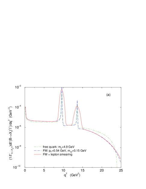
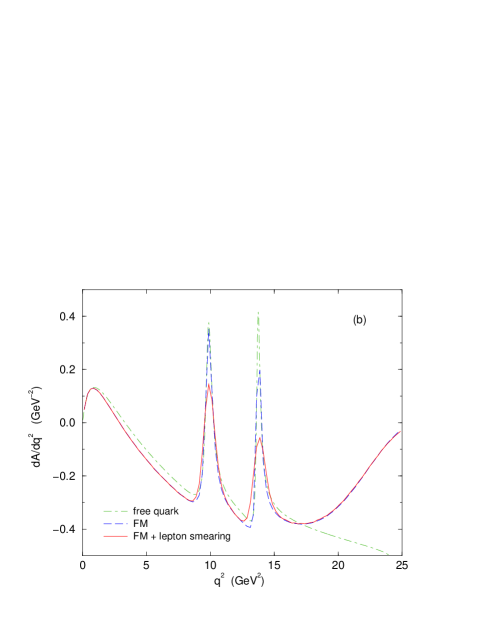
FIG. 1.: The distributions (a) $(1/\Gamma_{b\to X_{c}\ell\nu})d\Gamma(B\to X_{s}\ell^{+}\ell^{-})/dq^{2}$ and (b) $dA/dq^{2}$ showing the effects of fermi motion (FM) of the $b$ quark inside $B$ meson and of the leptonic smearing.

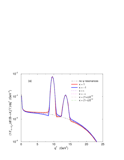
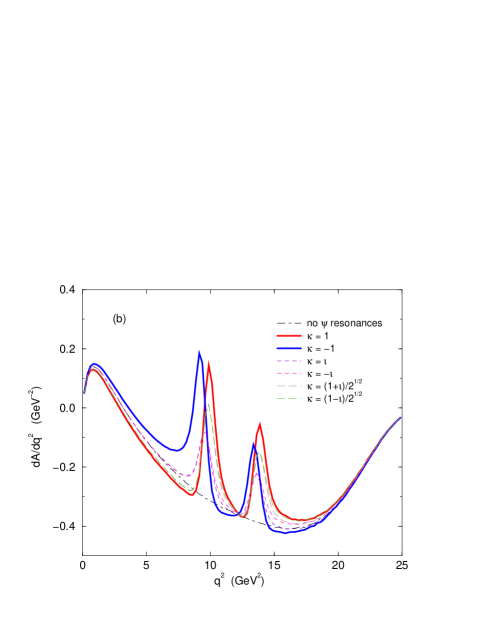
FIG. 2.: The distributions (a) $(1/\Gamma_{b\to X_{c}\ell\nu})d\Gamma(B\to X_{s}\ell^{+}\ell^{-})/dq^{2}$ and (b) $dA/dq^{2}$ showing the effects of varying the phase $\kappa$ between the $\psi$ and perturbative amplitudes.

IV Sensitivity to New Physics

We use the two-Higgs-doublet-model II (2HDMII) and a model-independent method to illustrate the sensitivities. We start with the 2HDMII, which is a popular extension of the SM and provides a minimal Higgs sector for supersymmetry. The extra contributions to the Wilson coefficients $C_{i}$ depend on the charged Higgs boson mass and $\tan\beta$. For clarity we list the coefficients $C_{7-10}(M_{W})$ here [3, 8, 12]:

$$C_{7}(M_{W}) = -\frac{A(x_{t})}{2}-\frac{A(x_{H})}{6\tan^{2}\beta}-B(x_{H})$$ (21)

$$C_{8}(M_{W}) = -\frac{D(x_{t})}{2}-\frac{D(x_{H})}{6\tan^{2}\beta}-E(x_{H})$$ (22)

$$C_{9}(M_{W}) = \frac{Y}{\sin^{2}\theta_{\rm w}}-4Z$$ (23)

$$C_{10}(M_{W}) = -\frac{Y}{\sin^{2}\theta_{\rm w}}$$ (24)

$$Y = C(x_{t})-F(x_{t})-\frac{x_{t}}{8\tan^{2}\beta}f_{5}(x_{H})$$ (25)

$$Z = C(x_{t})+\frac{G(x_{t})}{4}-\frac{x_{t}}{8\tan^{2}\beta}f_{5}(x_{H})-\frac{1}{72\tan^{2}\beta}f_{6}(x_{H})\;,$$ (26)

where

$$A(x) = x\biggr{[}\frac{8x^{2}+5x-7}{12(x-1)^{3}}-\frac{(3x^{2}-2x)\log x}{2(x-1)^{4}}\biggr{]}$$ (27)

$$B(x) = x\biggr{[}\frac{5x-3}{12(x-1)^{2}}-\frac{(3x-2)\log x}{6(x-1)^{3}}\biggr{]}$$ (28)

$$D(x) = x\biggr{[}\frac{x^{2}-5x-2}{4(x-1)^{3}}+\frac{3x\log x}{2(x-1)^{4}}\biggr{]}$$ (29)

$$E(x) = x\biggr{[}\frac{x-3}{4(x-1)^{2}}+\frac{\log x}{2(x-1)^{3}}\biggr{]}$$ (30)

$$C(x) = \frac{x}{8}\biggr{[}\frac{x-6}{x-1}+\frac{(3x+2)\log x}{(x-1)^{2}}\biggr{]}$$ (31)

$$F(x) = \frac{1}{4}\biggr{[}\frac{x}{1-x}+\frac{x\log x}{(x-1)^{2}}\biggr{]}$$ (32)

$$G(x) = -\frac{4}{9}\log x+\frac{-19x^{3}+25x^{2}}{36(x-1)^{3}}+\frac{x^{2}(5x^{2}-2x-6)\log x}{18(x-1)^{4}}$$ (33)

$$f_{5}(x) = \frac{x}{1-x}+\frac{x\log x}{(1-x)^{2}}$$ (34)

$$f_{6}(x) = \frac{38x-79x^{2}+47x^{3}}{6(1-x)^{3}}+\frac{(4x-6x^{2}+3x^{4})\log x}{(1-x)^{4}}$$ (35)

$$x_{t} = m_{t}^{2}/M_{W}^{2}\;,x_{H}=m_{t}^{2}/m_{H^{\pm}}^{2}\;.$$ (36)

We are now ready to investigate the effects of extra charged Higgs contributions to $C_{i}(M_{W})$ and in turns to the spectra of leptonic invariant mass and forward-backward asymmetry. Since 2HDMII always pushes $C_{7}(M_{W})$ more negative, the absolute value of $C_{7}^{\rm eff}$ increases and so does the rate of $b\to s\gamma$. Using the experimental rate from CLEO: $1\times 10^{-4}<BR(b\to s\gamma)<4.2\times 10^{-4}$ at 95%CL level [1], we limit the range of charged Higgs mass to be $m_{H^{\pm}}\gtrsim 400$ GeV for all $\tan\beta>1$. In Fig. 3, we show the invariant mass and forward-backward asymmetry for the 2HDMII with $m_{H}=400-800$ GeV in an increment of 100 GeV and $\tan\beta=1,10,20,30,$ and 40. Here we do not include the effects of fermi motion nor the leptonic smearing. It is clear that the results implied by various charged Higgs mass $m_{H^{\pm}}\gtrsim 400$ GeV cannot be easily distinguished from the SM.

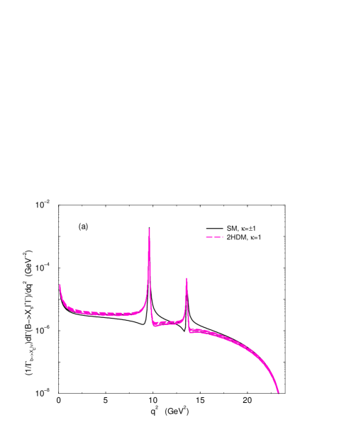
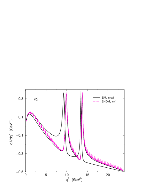
FIG. 3.: (a) Invariant mass and (b) forward-backward asymmetry for the two-higgs-doublet model II with $m_{H^{\pm}}=400-800$ GeV with an increment of 100 GeV and $\tan=1-40$. The two curves of the SM with $\kappa=\pm 1$ are also shown.

Next, we are going to use a model-independent method by varying $C_{i}(M_{W}),i=7,9,10$, hoping that it can cover a wide variety of models of new physics. We look at each of $C_{7}(M_{W}),C_{9}(M_{W})$, and $C_{10}(M_{W})$ while keeping the others at the SM value. We shall estimate the range beyond which the resulting spectra are distinguishable from the SM ones. We do not look at $C_{8}(M_{W})$ because $C_{8}^{\rm eff}(\mu)$ do not enter Eqs. (14) and (15) directly and therefore the limit on the range of $C_{8}(M_{W})$ is rather loose. We found that changing the values of $C_{7,9,10}(M_{W})$ only changes the normalization of the continuum part of the invariant mass spectrum, which is not easy to identify given the experimental uncertainties. Therefore, we concentrate on the forward-backward asymmetry. We confirm that the forward-backward asymmetry is more sensitive than the invariant mass spectrum to changes in $C_{7,9}(M_{W})$. However, for $C_{10}(M_{W})$ invariant mass spectrum appears to change more than the forward-backward asymmetry, but still only the normalization of the continuum changes. We shall discuss it in a moment.

First we look at $C_{7}(M_{W})$. We found that the forward-backward asymmetry is rather sensitive to $C_{7}(M_{W})$ at the small $q^{2}$ region. In Fig.  4, we show curves for $C^{\rm SM}_{7}(M_{W})\approx-0.2$, $C_{7}(M_{W})=0$, and $C_{7}(M_{W})=-0.4$ with $\kappa=\pm 1$. The region bounded by the SM curves of $\kappa=\pm 1$ shows more or less the uncertainty in prediction. We define a $C_{7}(M_{W})$ is distinguishable from the SM prediction when it has a significant region not overlapping with the SM region. As seen in Fig. 4, both $C_{7}(M_{W})=0,-0.4$ have a region outside the SM region. For

$$C_{7}(M_{W})\lesssim-0.4\;,\qquad{\rm or}\qquad C_{7}(M_{W})\gtrsim 0$$ (37)

the forward-backward asymmetry is further distinguishable from the SM one. However, one has to be careful about the range of $C_{7}(M_{W})$ shown in Eq. (37). We can apply the SM evolution to evaluate the corresponding range in $C_{7}^{\rm eff}(\mu=m_{b})$ and we obtain $C_{7}^{\rm eff}(m_{b})<-0.45$ or $C_{7}^{\rm eff}(m_{b})>-0.18$, respectively. The first range $C_{7}^{\rm eff}(m_{b})<-0.45$ is already inconsistent with the experimental rate of $b\to s\gamma$ (the allowed range of $|C_{7}^{\rm eff}(m_{b})|\approx 0.2-0.4$.) The second range, on the other hand, has some overlaps with the experimentally allowed range.

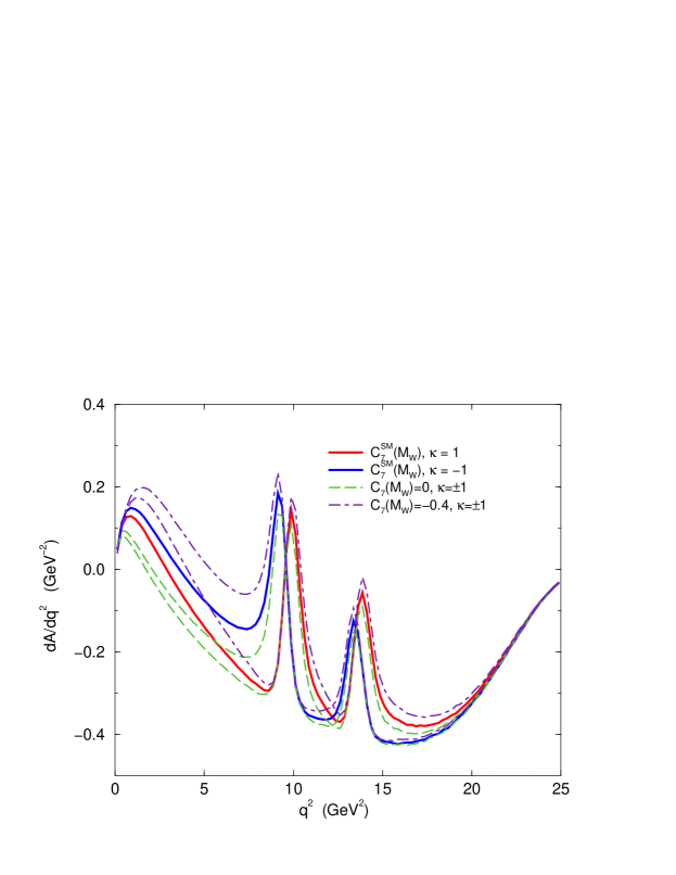
FIG. 4.: The forward-backward asymmetry predicted for $C^{\rm SM}_{7}(M_{W})$, $C_{7}(M_{W})=0$, and $C_{7}(M_{W})=-0.4$ with $\kappa=\pm 1$. The upper curve of each set is for $\kappa=-1$ while the lower has $\kappa=1$.

We now look at $C_{9}(M_{W})$. The SM value for $C_{9}^{\rm SM}(M_{W})\approx 1.6$. Using the forward-backward asymmetry we found that

$$C_{9}(M_{W})\lesssim 0\;,\qquad{\rm or}\qquad C_{9}(M_{W})\gtrsim 4\;,$$ (38)

is needed in order that the resulting spectra is sufficiently different from the SM curves, as shown in Fig. 5. In the SM, $C_{10}(M_{W})\approx-4.5$. Since the forward-backward asymmetry $dA/dq^{2}$ is roughly proportional to $C_{10}(M_{W})$, as indicated by the numerator of Eq. (15), therefore the asymmetry will not change significantly unless $C_{10}(M_{W})$ changes sign. We found that we need a rather large change in $C_{10}(M_{W})$ in order for the forward-backward asymmetry to be distinguishable from the SM curves. We found, as shown in Fig. 6,

$$C_{10}(M_{W})\lesssim-8\;,\qquad{\rm or}\qquad C_{10}(M_{W})\gtrsim-1\;$$ (39)

is needed. However, this difference is only marginal and only at the large $q^{2}$ region, where the event rate is relatively low.

Overall, we have found that we need a rather large change in $C_{9,10}(M_{W})$ in order to make the forward-backward asymmetry distinguishable from the SM prediction. Although $C_{7}({M_{W}})$ does not need to change a lot for the effect to be seen, the sensitivity range is, however, severely limited by the experimental rate of $b\to s\gamma$.

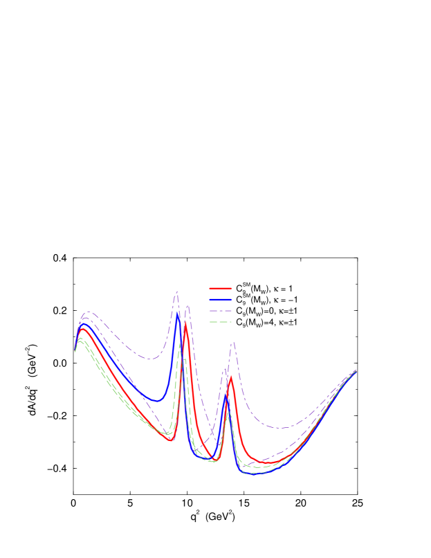
FIG. 5.: The forward-backward asymmetry predicted for $C^{\rm SM}_{9}(M_{W})$, $C_{9}(M_{W})=0$, and $C_{9}(M_{W})=4$ with $\kappa=\pm 1$. The upper curve of each set is for $\kappa=-1$ while the lower has $\kappa=1$.

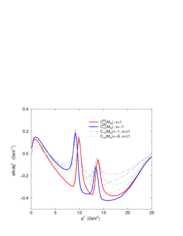
FIG. 6.: The forward-backward asymmetry predicted for $C^{\rm SM}_{10}(M_{W})$, $C_{10}(M_{W})=-1$, and $C_{10}(M_{W})=-8$ with $\kappa=\pm 1$. The upper curve of each set is for $\kappa=-1$ while the lower has $\kappa=1$.

V Conclusions

In this report, we have studied the sensitivities of invariant mass and forward-backward asymmetry of the lepton pair in the decay $B\to X_{s}\ell^{+}\ell^{-}$ to changes in the Wilson coefficients $C_{7,9,10}(M_{W})$, under both the theoretical uncertainties, including the effect of $b$-quark fermi motion inside $B$ meson and the unknown phase between the perturbative amplitude and the long-distance $\psi$ amplitudes, as well as the experimental uncertainty of the measurement of lepton momenta. All these uncertainties make the SM prediction become a broad “region” that only when new physics predictions go beyond this region can one say the spectrum is sensitive to new physics. We found that the sensitivity of the lepton forward-backward asymmetry is rather weak to changes in $C_{9,10}(M_{W})$. Only when $C_{9,10}(M_{W})$ change substantially will the asymmetry be distinguishable from the SM prediction. For $C_{7}(M_{W})$ the lepton forward-backward asymmetry is more sensitive but, however, a large part of the sensitivity range is already ruled out by the $b\to s\gamma$ rate.

This work was supported by the DOE under contracts No. DE-FG03-91ER40674 and by the Davis Institute for High Energy Physics.

REFERENCES

• [1] M.S. Alam et al. (CLEO Coll.), Phys. Rev. Lett. 74, 2884 (1995).
• [2] A. Ali, T. Mannel, and T. Morozumi, Phys. Lett. B273, 505 (1991); D. Liu, Phys. Rev. D52, 5056 (1995); Melikhov, N. Nikitin, and S. Simula (Rome, ISS), Phys. Lett. B430, 332 (1998).
• [3] G. Buchalla, A. Buras, and M. Lautenbacher, Rev. Mod. Phys. 68, 1125 (1996).
• [4] N. Deshpande, J. TrampetiΔ‡, and K. Panose, Phys. Rev. D39, 1461 (1989);C. Lim, T. Morozumi, and A. Sanda, Phys. Lett. B218, 343 (1989).
• [5] P. O’Donnell and H. Tung, Phys. Rev. D43, 2067 (1991).
• [6] G. Altarelli et al., Nucl. Phys. B208, 365 (1982).
• [7] B. Grinstein, R. Springer, and M. Wise, Nucl. Phys. B339, 269 (1990).
• [8] A. Ali et al., Phys. Rev. D55, 4105 (1997); A. Ali and G. Hiller, hep-ph/9807418.
• [9] Z. Ligeti and M. Wise, Phys. Rev. D53, 4937 (1996).
• [10] J. Chay, H. Georgi, and B. Grinstein, Phys. Lett. B247, 399 (1990).
• [11] CLEO Collaboration, R. Balest et al., Phys. Rev. D52, 2661 (1995).
• [12] J. Hewett and J. Wells, Phys. Rev. D55, 5549 (1997).