The Gross–Llewellyn Smith Sum Rule in the Analytic Approach to Perturbative QCD
Abstract
We apply analytic perturbation theory to the Gross–Llewellyn Smith sum rule. We study the evolution and the renormalization scheme dependence of the analytic three-loop QCD correction to this sum rule, and demonstrate that the results are practically renormalization scheme independent and lead to rather different evolution than the standard perturbative correction possesses.
PACS: 11.10.Hi; 11.55.Hx; 12.38.Cy; 13.15+g
I Introduction
At present two deep inelastic scattering (DIS) sum rules, the Gross–Llewellyn Smith (GLS) [1] and the polarized Bjorken sum rule [2], give the possibility of extracting the value of the strong coupling constant from experimental data, in particular, at low momentum transfer, , down to (see, e.g., Refs. [3, 4]). Comparison of these values of with other accurate values, such as those obtained from the decay widths of the -lepton and the -boson into hadrons, is an important test of the consistency of QCD. Clearly what are required are reliable theoretical relations between physically observable quantities and the strong coupling constant . At low scales, there are significant theoretical uncertainties, which come, firstly, from a truncation of the series obtained from perturbation theory (PT), which leads to a significant renormalization scheme (RS) ambiguity, and, secondly, from poorly understood nonperturbative effects (see, e.g., Refs. [5, 6] for a review). In this paper we apply the method proposed in Refs. [7, 8] (see also Refs. [9, 10]), the so-called analytic perturbation theory (APT), to study the GLS sum rule, continuing our investigation of the APT approach initiated in Refs. [11, 12]. This method takes into account the fundamental principle of causality, which in the simplest cases is reflected in the form of -analyticity of the Källn–Lehmann type. The standard renormalization group resummation violates this required analytic structure, and unphysical singularities such as a ghost pole appear. The APT approach maintains the causal properties and removes all unphysical singularities by incorporating nonperturbative terms (for the number of flavors occurring in nature) to secure the required analytic properties. These nonperturbative terms can be presented as power corrections and their appearance is not inconsistent with the operator product expansion [13].
It is familiar that the QCD correction to the GLS sum rule is expressed as an expansion in powers of that allows one, in principle, easily to obtain a value for the running coupling constant. Before going into detailed considerations, let us demonstrate the difference between the standard PT and APT running coupling constants in the two-loop level. The two-loop analytic running coupling constant can be written in the form of a sum of the standard perturbative part and additional terms which compensate for the contributions of unphysical singularities, the ghost pole and a cut arising from the “log-of-log” dependence. The difference may be transparently shown by using the approximate formulae for the two-loop analytic running coupling given in Ref. [8]
| (1) |
where is the one-loop coefficient of the -function corresponding to active quarks, and, for four active flavors, The PT running coupling constant is obtained by integration of the renormalization group equation with the two-loop -function.
The difference between the APT and PT functions is illustrated in Fig. 1 over a wide range of , . The curves in the figure correspond to various values of the QCD scale parameter for four active flavors. Fig. 1 shows that the expression (1), represented by dotted lines, approximates the exact two-loop analytic coupling (solid lines) rather well for . Comparing the evolution of the QCD running coupling constant obtained from APT to that given by PT (dashed lines), one can see that the difference between the shapes of the APT and PT running coupling constants becomes significant at low -scales, . This fact stimulated applications of the modified perturbation theory with correct analytic properties, APT, for various physical processes (see, e.g., Refs. [11, 14]). Here, we consider the GLS sum rule in the framework of the APT approach. As has been demonstrated in Ref. [15] by using the Deser-Gilbert-Sudarshan representation for the virtual forward Compton amplitude [16] (see also Ref. [17]), the moments of the structure functions are analytic functions in the complex -plane with a cut along the negative real axis. On the other hand, the conventional renormalization group resummation does not support these analytic properties and the influence of requiring these properties to hold in the DIS description has not been studied. Here, we perform this investigation, by applying the APT method, which gives the possibility of combining the renormalization group resummation with correct analytic properties of the QCD correction to the GLS sum rule. In Sec. II we start by describing the GLS sum rule in the PT and APT approaches and compare the evolution of the APT and PT predictions. In Sec. III we consider in detail the RS dependence of the results. Summarizing comments are given in Sec. IV.
II The GLS sum rule within APT
The GLS sum rule predicts the value of the integral over all of the non-singlet structure function measured in neutrino- and antineutrino-proton scattering
| (2) |
In the quark-parton level, which is appropriate for , the GLS sum rule should equal three. Therefore, for fixed the integral (2) can be conveniently written as
| (3) |
where the QCD correction, , in principle, contains perturbative and nonperturbative parts. To begin, we concentrate on the perturbative contribution to , considering in turn standard PT and APT methods and postponing until later a discussion of the possible influence of higher twist (HT) effects, which remain poorly understood. In this connection it is interesting to note from the result of the fit to the revised CCFR data [18] presented in Refs. [19] that the higher-twist contributions are small in the region and can have a sign-alternating character.
The standard perturbative part of the GLS sum rule correction is known up to the three-loop level for massless quarks in the MS-like renormalization schemes with the number of active quarks fixed,
| (4) |
The PT running coupling constant is obtained by integration of the renormalization group equation with the three-loop -function. The coefficients and are given in Ref. [20] in the renormalization scheme. Therefore, the perturbative QCD correction to the GLS sum rule is represented in the form of a power series in and, at first glance, the value of can be easily extracted if the value of is experimentally known. In the region , one believes PT with its renormalization-group improvement is still valid. We should note that different regions of the integration in Eq. (2) at fixed values of , in principle, correspond to different numbers of active quarks, ; arguments have been given in Ref. [21] to select one or another value of . Experimental measurements of the GLS sum rule are made in a region of where one believes that four light flavors are relevant. At present, there is no regular and consistent method of including threshold effects for the GLS sum rule. In the following analysis, we will first take to obtain results in the standard renormalization scheme, and then consider RS dependence.
The QCD correction with correct analytic properties can be written in the form of a spectral representation
| (5) |
where we have introduced the spectral function, which is defined as the discontinuity of : . If we calculate now the spectral function perturbatively, we get an expression for , which has the correct analytic properties and therefore no unphysical singularities. Consequently, we write the three-loop APT approximation to as follows
| (6) |
where the coefficients and are the same as in Eq. (4) and the functions are derived from the spectral representation and correspond to the discontinuity of the -th power of the PT running coupling constant
| (7) |
The function defines the APT running coupling constant, , which in the one-loop order is given by
| (8) |
As can be seen from Eq. (6), the first term of the expansion is , but the following terms are not representable as powers of unlike in the PT case. There are approximate expressions, like Eq. (1), for higher loop corrections in Eq. (6), which have rather simple forms, which can be derived by using a method of subtracting unphysical singularities [22]. For instance, for , the approximate formula is
| (9) |
where for four active flavors and .
To illustrate the difference between the convergence properties of the PT expansion (4) and the APT series (6) we use the recent result of the CCFR Collaboration (CCFR’97) [23, 24]: at , which is consistent with the result of a previous CCFR analysis (CCFR’93) [25], at . The central value of corresponds to the value of the QCD correction and the successive terms of the PT series (4) respectively constitute 65.1%, 24.4% and 10.5% of the total. At the same time, the corresponding contributions to the APT series (6) make up 75.7%, 20.7% and 3.6% of the total. The convergence of the APT series seems to be somewhat better behaved than is that of the PT expansion at such small .
The same may be seen from Fig. 2, where is shown as a function of the QCD running coupling constant in the PT and APT approaches. As outlined above, in the PT case, the function is an explicit function of the PT running coupling constant and in the one-loop approximation is represented by a straight line in Fig. 2, as a parabola in the two-loop case, and as a cubic curve in the three-loop one. At sufficiently large values of , the difference between the 1-, 2-, and 3-loop PT predictions becomes large. An inclusion of the higher-twist term with the value recommended by the Particle Data Group, [26] (see Refs. [27, 28] for additional details), also significantly changes the behavior, as is apparent from the figure. Note that the coincidence of the one-loop PT and APT curves in Fig. 2 does not mean that the PT and APT approaches are physically identical, this is simply a matter of the linear form of the one-loop approximation; the behavior of the PT and APT running coupling constants are rather different [see Eq. (8)]. In the APT case, the contribution of the higher loop corrections is not so large as in the PT one and the corresponding curves in Fig. 2 are quite close to the linear function, and, especially, there is very little difference between the 2-loop and 3-loop results. The horizontal lines in Fig. 2 correspond to central values from experimental data at different low values of : [29], [25], [23, 24]. The intersection of one of these lines with a given theoretical curve gives the value of for that value of in that theoretical description. It will be seen that stability of the theoretical curve at a few GeV2 is required in order to extract a reliable value of or the QCD scale parameter .
Consider the evolution of the GLS sum rule. In Ref. [30], the low- dependence of GLS sum rule has been evaluated by combining measurements of the CCFR’93 data with data from other DIS experiments. Preliminary updated analysis with CCFR’97 data was presented in Refs. [23, 24]. The analysis of the GLS sum rule based on the Jacobi polynomial expansion has been given in Ref. [31], and for new CCFR’97 data has been examined in Ref. [32]. The very recent CCFR/NuTEV result for the GLS integral is presented in Refs. [33, 34, 35]. The three values of the GLS integral at , , and GeV2 are in good agreement with the old result [30], but the value at GeV2 is larger, which corresponds to a smaller value of the QCD correction to GLS sum rule, although consistent within errors (see also Fig. 4). Note that the value [34] gives a very small value of the scale parameter MeV. The choice of normalization point influences the value of the parameter , but does not change the general picture of there being a difference between the APT and PT results for low scales. To study this difference we take the relevant value of MeV. That practically means the normalization on the value [34] that gives MeV. This value of the scale parameter is quite realistic and agrees well with the results of the fits to the structure function from the CCFR’97 data, for example, with the two-loop result MeV [18] and with the three-loop value MeV [19]. Since the difference between the PT and APT forms of the QCD corrections is of order , both these functions will coincide in the asymptotic region, where the perturbative approximation is valid.
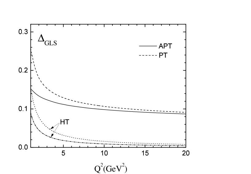
The comparison between the evolution in the APT and PT approaches is shown in Fig. 3, where the QCD correction to the GLS sum rule is plotted for the perturbative part (solid curve for APT and dashed for PT approach) and separately for the HT term given by two different estimations for the coefficients in the form (dash-dotted line) and (dotted line) taken from Refs. [27, 28], respectively. This figure demonstrates that there is an essential difference between PT and APT evolutions for low . Instead of a rapidly changing function with unphysical singularities as occurs in the PT case, we get a slowly changing function in the APT approach.
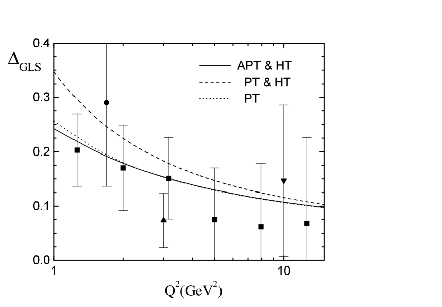
In Fig. 4 we plot the full contribution to the QCD correction with the perturbative part, calculated in the PT and APT approaches, and the HT part taken in the form as discussed above [26]. We also plot the data, indicated by squares, of the recent CCFR/NuTeV analysis [33, 34] where the behavior of the GLS integral has been evaluated at values of between and , as well as older data. The dotted curve represents the PT result without HT effects. At high scales, the PT and APT results agree closely with each other, both including the HT effects and without them, whereas at low scales, the difference between the PT and APT behaviors becomes significant. At the same time, for , the PT prediction without the HT term practically coincides with the APT curve including the HT term. Cancellation between the additional APT terms beyond the standard PT prediction and the HT terms can explain the fact that attempts to extract the HT effect from the CCFR’97 experimental data give a rather small value, even poorly determining the sign of the HT contribution (see, for detail, Ref. [19]). Note also that in the analysis of Refs. [23, 24] the HT contribution to the QCD correction for the GLS sum rule is taken to be given by the form ; however, in the subsequent papers [33, 34, 35], the HT term has been taken to be smaller, . Thus, the comparison of the APT and PT predictions with experimental data, as is demonstrated in Fig. 4, cannot give a definite conclusion since there are large experimental errors and the value of the HT corrections is very uncertain.
We have considered the evolution of the GLS sum rule in the customary renormalization scheme. In general, it is not sufficient to obtain a result in some scheme, but rather it is important to study its RS stability over some acceptable domain. The RS dependence of the GLS sum rule based on the PT approach has been studied in Ref. [21]. In the next section we consider the RS stability of the APT results.
III Renormalization scheme dependence
A truncation of a perturbative expansion leads to uncertainties in the theoretical predictions arising from the RS dependence of the partial sum of the series. At low momentum scales these uncertainties may become very large (see, for example, an analysis in Ref. [38]). A physical quantity, in our case the QCD correction to the GLS sum rule, has to be invariant under a change of RS, when the coupling constant transforms as follows ()
| (10) |
In the new RS, the QCD correction is represented as
| (11) |
where the coefficients and are RS dependent and have the transformation law
| (12) | |||||
| (13) |
In the three-loop level there are two process-dependent invariants under the RS-transformation (10) [39]
| (14) | |||||
| (15) |
where , and are the coefficients of the three-loop -function
| (16) |
The coefficient , as well and , depends on RS, and, because of the first equation in (12), the scale parameter transforms as follows [40]: . In terms of the scale parameter , the three-loop perturbative running coupling in any RS obeys the equation
| (17) |
where
| (18) | |||||
| (19) |
Thus, any RS taken from the -like schemes can be characterized by two parameters, which we choose here to be and . To calculate the second RS invariant one can use the coefficients in the scheme, which for are .
In the framework of the conventional approach there is no solution of the RS dependence problem apart from calculating many further terms in the asymptotic PT expansion, and there is no fundamental principle upon which one can choose one or another preferable RS. Usually, one uses a class of ‘natural’ or ‘well-behaved’ RSs, which are defined by the so-called cancellation index criterion [41], according to which the degree of cancellation between the different terms in the second RS-invariant are not too large, as measured by the cancellation index
| (20) |
By taking some maximum value of the cancellation index one can investigate the stability of predictions for those RSs with . In the case of the -scheme the value of the cancellation index for the GLS sum rule is . Taking into account that the scheme is commonly used, we will consider this value as a boundary for the class of ‘natural’ schemes. In addition we will compare our results with predictions given by optimized schemes based on the principle of minimal sensitivity (PMS) [39] and the method of effective charge (ECH) [42]. (See also applications in [21, 43, 44]).
It should be stressed that the large value of the cancellation index for four active quark flavors does not mean that the coefficients from which the second RS invariant is constructed are huge, only that is small, . In this special case the value of is very sensitive to the value of ; for example, for , this invariant becomes and the cancellation index becomes significantly reduced. At the same time, the absolute values of the coefficients that construct the second RS invariant (15) are smaller for than for , however, . Perhaps, in this situation, it is more convenient to introduce as the corresponding index, which will define the class of ‘natural’ RSs, the sum of the absolute values of the terms in , without the denominator in Eq. (20). The numerical parameter introduced in such a way will practically define the same region in the -plane, without changing significantly with changing , and, therefore, more adequately describing the situation.
Let us briefly discuss results of the ECH and PMS approaches. For the ECH scheme the parameters are and, therefore, . The transformation from the scheme to the ECH scheme is performed with the parameters in Eq. (10) and . The system of equations for getting the PMS optimal prescription consists of four equations. These are Eqs. (15) and (17) complemented by the following two equations:
| (21) | |||
| (22) |
where
| (23) |
In the PMS optimization procedure the coefficients , and become dependent and, therefore, have to be adjusted for each different value of .
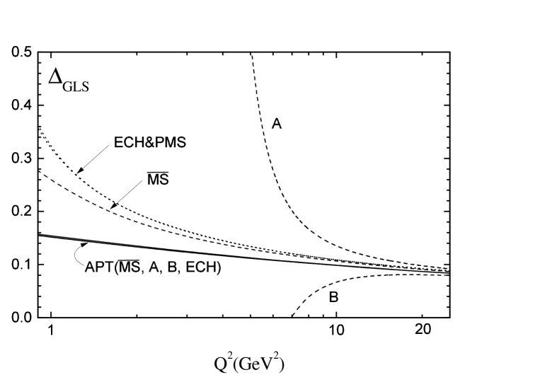
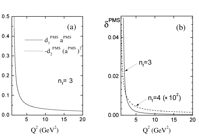
We present our results in Fig. 5, where the QCD correction is plotted as a function of in different RS. The schemes A and B have the same cancellation index as in the scheme, , and are defined by the following values of the parameters: , and , . The dotted curves present the ECH and PMS predictions, which are very close to each other. This is because the PMS coefficients and are found for four active quark flavors to be small numerically in the region under consideration, . Behaviors of these coefficients as functions of are shown separately in Fig. 6.
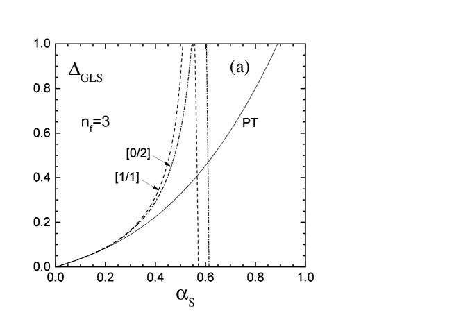
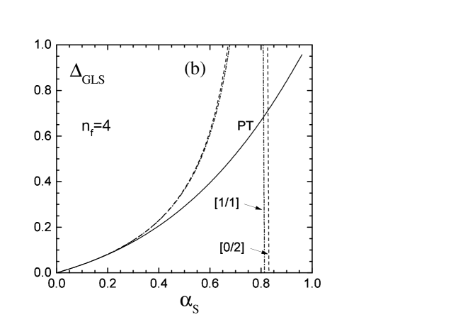
As it has been mentioned above, there are no strong arguments to fix the definite number of active quark flavors for the integral (2) to be . Therefore, we have also considered the case . The ECH and PMS prescriptions gave again results that are very close to each other. However, the reason is no longer that the PMS coefficients and are very small, but that there is a strong cancellation between the last two terms in the expression for the QCD correction with . This fact is demonstrated in Fig. 7, where (a) shows the quadratic (solid line) and cubic (dotted line) contributions to for . The sum of these contributions is shown in Fig. 7 (b) for (solid line) and for (dashed line).
The APT predictions for the , A, and B schemes turn out to be stable for the whole interval of momenta and appears as a wide solid line in Fig. 5. It should be stressed that the optimized RS constructions in the framework of PT do not maintain the correct causal properties, however, to avoid this difficulty, they can be modified in the sense of APT. In Fig. 5 we plot the analytic ECH result, which, of course, is different from the perturbative one and practically coincides with the other APT curves for the , A, and B schemes.
The sensitivity of the PT predictions to the RS dependence can be reduced by applying the Pad approximation (PA) [45]. However, in the case under consideration, this approach can lead to some difficulties. In Fig. 8 we plot two possible Pad approximants and in the three-loop order for versus . This figure demonstrates that the PA leads to unphysical singularities in the region of small momenta that violate the causal properties and prevents us from considering the method of PA as a systematic approach. In contrast, the APT results for the , A, B, and ECH schemes lead to stable predictions for the whole interval of momentum, which practically coincide with each other, and, therefore, the APT description turns out to be practically RS independent.
IV Summary and conclusion
We have considered the GLS sum rule by using the APT approach, which maintains the causal properties and, in contrast to PT, does not lead to any unphysical singularities. Taking into account the analytic properties of the moments of the deep inelastic structure functions, we have obtained an analytically improved theoretical description of the GLS sum rule. We have shown that the convergence properties of the APT expansion are better than are those in the standard PT description. We have demonstrated further that there is a significant difference between the evolution in the PT and APT approaches for low scales. We have also analyzed the GLS sum rule taking into account the higher-twist contribution. The APT power corrections have a sign opposite to that of the typically-used higher-twist term [26] and, numerically, there is an effective cancellation between these two corrections.
In this paper we have found that in the framework of APT the theoretical prediction to the GLS sum rule becomes practically renormalization scheme independent starting from the three-loop level. A similar statement has been made for the annihilation into hadrons [46] and for the semileptonic inclusive decay of the lepton [47]. A corresponding analysis of the Bjorken sum rule is presented in Ref. [14]. Thus, the APT approach gives a systematic method of reducing the RS ambiguity significantly and leads to practically unique predictions for physical quantities. It should be stressed that our analysis shows that there is serious doubt concerning the conjecture that, in spite of the large values of at low , the conventional three-loop PT predictions for the GLS sum rule are reliable (see, e.g., [35]). The proximity of PT predictions in the scheme to predictions obtained in the optimal schemes seems to possess no significance for any process at small momentum transfer and cannot be considered a guarantee of RS independence of the results.
Unfortunately, at present, the experimental situation for the GLS sum rule, with its large errors, does not allow us to come to a reliable conclusion that the APT description is preferable to the PT one. However, from the theoretical point of view, the remarkable properties of the APT approach, for example, the maintenance of causality and the higher-loop and renormalization-scheme stability for the whole interval of momenta, create a basis for preferring the application of this new technique.
Acknowledgement
The authors would like to thank L. Gamberg, A. L. Kataev, and S. M. Mikhailov for useful discussions and interest in this work, O. Nachtmann who brought the paper [15] to our attention, and J. H. Kim for useful discussion of the CCFR/NuTeV data.
Partial support of the work by the US National Science Foundation, grant PHY-9600421, by the US Department of Energy, grant DE-FG-03-98ER41066, by the University of Oklahoma, and by the RFBR, grant 96-02-16126 is gratefully acknowledged.
REFERENCES
- [1] D. J Gross and C. H. Llewellyn Smith, Nucl. Phys. B 14, 337 (1969).
- [2] J. D. Bjorken, Phys. Rev. 148 (1966) 1467; Phys. Rev. D 1, 1376 (1970).
- [3] P. N. Burrows et al., SLAC-PUB-7371, in New Directions for High-Energy Physics , Proceedings of Snowmass Workshop 96, edited by D. G. Cassel, L. Trindle Gennari, R. H. Siemann (Stanford Linear Accelerator Center, 1997), hep-ex/9612012.
- [4] M. Albrow et al., in New Directions for High-Energy Physics , Proceedings of Snowmass Workshop 96, edited by D. G. Cassel, L. Trindle Gennari, R. H. Siemann (Stanford Linear Accelerator Center, 1997), hep-ph/9706470.
- [5] M. A. Shifman, Int. J. of Mod. Phys. A 10, 235 (1995).
- [6] J. Fischer, Int. J. of Mod. Phys. A 12, 3625 (1997).
- [7] D. V. Shirkov and I. L. Solovtsov, JINR Rap. Comm. 1996. No. 2[76]-96, 5 (1996), hep-ph/9604363.
- [8] D. V. Shirkov and I. L. Solovtsov, Phys. Rev. Lett. 79, 1209 (1997).
- [9] K. A. Milton and I. L. Solovtsov, Phys. Rev. D 55, 5295 (1997).
- [10] D. V. Shirkov, in QCD 97: 25th Anniversary of QCD, Proceedings of the QCD 97 Euroconference, edited by S. Narison [Nucl. Phys. B (Proc. Suppl.) 64, 106 (1998)].
- [11] K. A. Milton, I. L. Solovtsov, and O. P. Solovtsova, Phys. Lett. B 415, 104 (1997).
- [12] K. A. Milton and O. P. Solovtsova, Phys. Rev. D 57, 5402 (1998).
- [13] G. Grunberg, in ‘97 QCD and High Energy Hadronic Interactions, Proceedings of the XXXIInd Rencontres de Moriond, Les Arcs, Savoie, France, 1997, edited by J. Trn Thanh Vn (Editions Frontieres, 1997), p. 337; hep-ph/9705290.
- [14] K. A. Milton, I. L. Solovtsov, and O. P. Solovtsova, OKHEP-98-03, to be published in Phys. Lett. B; talk given at ICHEP98, Vancouver, Canada, 1998; hep-ph/9808457.
- [15] W. Wetzel, Nucl. Phys. B 139, 170 (1978).
- [16] S. Deser, W. Gilbert, and E. C. G. Sudarshan, Phys. Rev. 115, 731 (1959); ibid 117, 266 (1960).
- [17] Ashok suri, Phys. Rev. D 4, 570 (1971).
- [18] CCFR/NuTeV Collaboration, W. G. Seligman et al., Phys. Rev. Lett. 79, 1213 (1997).
- [19] A. L. Kataev, A. V. Kotikov, G. Parente, and A. V. Sidorov, in ‘97 QCD and High Energy Hadronic Interactions, Proceedings of the XXXIInd Rencontres de Moriond, Les Arcs, Savoie, France, 1997, edited by J. Trn Thanh Vn (Editions Frontieres, 1997), p. 355; in QCD 97: 25th Anniversary of QCD, Proceedings of the QCD 97 Euroconference, edited by S. Narison [Nucl. Phys. B (Proc. Suppl.) 64, 138 (1998)]; Phys. Lett. B 417, 374 (1998).
- [20] S. A. Larin and J. A. M. Vermaseren, Phys. Lett. B 259, 315 (1991).
- [21] J. Chyla and A. L. Kataev, Phys. Lett. B 297, 385 (1992).
- [22] I. L. Solovtsov, paper in preparation.
- [23] CCFR/NuTeV Collaboration, P. Spentzouris, in Deep Inelastic Scattering and QCD (DIS 97), 5th International Workshop, Chicago, 1997, edited by Jos Repond and Daniel Krakauer (AIP, Woodbury, N.Y.), 1997, p. 409; and website http://www.hep.anl.gov/dis97/ .
- [24] CCFR/NuTeV Collaboration, Jaehoon Yu, in ‘97 QCD and High Energy Hadronic Interactions, Proceedings of the XXXIInd Rencontres de Moriond, Les Arcs, Savoie, France, 1997, edited by J. Trn Thanh Vn (Editions Frontieres, 1997), p. 349.
-
[25]
CCFR Collaboration, W. C. Leung et al.,
Phys. Lett. B 317, 655 (1993);
CCFR Collaboration, M. Shaevitz et al., Nucl. Phys. B (Proc. Suppl.) 38, 188 (1995). - [26] Particle Data Group, Eur. Phys. J. C 3, 1 (1998); and PDG website http://pdg.lbl.gov/.
- [27] I. I. Balitsky, V. M. Braun, and A. V. Kolesnichenko, Phys. Lett. B 242, 245 (1990); Phys. Lett. B 318, 648 (E) (1993).
- [28] G. G. Ross and R. G. Roberts, Phys. Lett. B 322, 425 (1994).
- [29] IHEP-JINR Neutrino Collaboration, L. S. Barabash el al., Preprint JINR E1-96-308, hep-ex/9611012.
- [30] CCFR Collaboration, D. A. Harris et al., FERMILAB Conf-95/144, hep-ex/9506010.
- [31] A. L. Kataev and A. V. Sidorov, Proc. of the Eighth Int. Seminar Quarks’94, Vladimir, Russia, World Scientific Publ. Co., 1995, p. 288; hep-ph/9405254; Phys. Lett. B 331, 179 (1994).
-
[32]
M. V. Tokarev, A. V. Sidorov,
Nuovo Cim. 110A, 1401 (1997), hep-ph/9707438;
A. V. Sidorov, Phys. Lett. B 389, 379 (1996). - [33] CCFR/NuTeV Collaboration, Jaehoon Yu, FERMILAB-CONF-98-198-E, talk given at XXXIIIrd Rencontres de Moriond: QCD and High Energy Hadronic Interactions, Les Arcs, France, 1998, hep-ex/9806030; FERMILAB-CONF-98-199-E, talk given at 6th International Workshop on Deep Inelastic Scattering and QCD (DIS 98), Brussels, Belgium, 1998, hep-ex/9806031.
- [34] CCFR/NuTev Collaboration, Jaehoon Yu, talk given at ICHEP’98, Vancouver, Canada, 1998; and website http://ichep98.triumf.ca/ .
- [35] CCFR/NuTev Collaboration, J. H. Kim, D. A. Harris et al., hep-ex/9808015.
- [36] CHARM Collaboration, F. Bergsma et al., Phys. Lett. 123B, 269 (1983).
- [37] CCFR Collaboration, F. S. Oltman et al., Z. Phys. C 53, 51 (1992).
- [38] P. A. Ra̧czka and A. Szymacha, Phys. Rev. D 54, 3073 (1996).
- [39] P. M. Stevenson, Phys. Rev. D 23, 2916 (1981).
- [40] W. Celmaster and R. J. Gonsalves, Phys. Rev. D 20, 1420 (1979).
- [41] P. A. Ra̧czka, Z. Phys. C 65, 481 (1995).
- [42] G. Grunberg, Phys. Rev. D 29, 2315 (1984).
- [43] A. C. Mattingly and P. M. Stevenson, Phys. Rev. D 49, 437 (1994).
- [44] A. L. Kataev, V. V. Starshenko, Mod. Phys. Lett. A 10, 235 (1995).
- [45] S. J. Brodsky, J. Ellis, E. Gardi, E. Karliner, and M. A. Samuel, Phys. Rev. D 56, 6980 (1997) and references therein.
- [46] I. L. Solovtsov and D. V. Shirkov, hep-ph/9711251.
- [47] K. A. Milton, I. L. Solovtsov, and V. I. Yasnov, OKHEP-98-01, hep-ph/9802282.