Higgs Decay into Gluons up to ${\cal O}(\alpha_{s}^{3}G_{F}m_{t}^{2})$

Abstract

The decay of the Standard Model Higgs boson in the intermediate-mass range into gluons is considered where special emphasis is put on the influence of the leading electroweak corrections proportional to $G_{F}m_{t}^{2}$. An effective Lagrangian approach is used where the top quark is integrated out. The evaluation of the coefficient function is performed using two different methods. The first one is concerned with the direct evaluation of the vertex diagrams and the second method is based on a low-energy theorem. In a first step the tools needed for the computation are provided namely the renormalization constants of the QCD Lagrangian are computed up to ${\cal O}(\alpha_{s}^{2}G_{F}m_{t}^{2})$. Also the decoupling constants for the strong coupling constant $\alpha_{s}$ and the light quark masses relating the quantities of the full theory to the corresponding quantities of the effective one are evaluated up to order $\alpha_{s}^{2}G_{F}m_{t}^{2}$.

PACS numbers: 12.15.Lk, 12.38.Bx, 12.38.-t, 14.80.Bn

I Introduction

The Higgs boson is the only not yet discovered particle of the Standard Model of elementary particle physics. Up to now only lower bounds on its mass of $M_{H}\,\hbox to0.0pt{\lower 3.5pt\hbox{$\mathchar 0\relax\sim$}\hss}\raise 1.0pt\hbox{$>$}\,89.8$ GeV [1] could be derived from the lack of observation at LEP 1 and LEP 2. Through the virtual presence of the Higgs boson in loop diagrams it is also possible to set indirect limits on $M_{H}$ with the help of the precision data collected at LEP, SLC and Tevatron. Currently they read $M_{H}=84^{+91}_{-51}$ GeV with an upper limit of $280$ GeV at 95 % C.L. [2]. These numbers suggest that a Higgs boson in the so-called intermediate-mass range, i.e. $M_{H}\,\hbox to0.0pt{\lower 3.5pt\hbox{$\mathchar 0\relax\sim$}\hss}\raise 1.0pt\hbox{$<$}\,2M_{W}$ where $M_{W}$ is the mass of the $W$ boson, is an attractive candidate. In this paper we will therefore consider such a Higgs boson and compute corrections to its gluonic decay rate.

Comprehensive reviews concerning the properties of the Higgs boson are given in [3, 4]. The dominant decay mode of an intermediate-mass Higgs boson is the one into bottom quarks. The QCD corrections are known up to ${\cal O}(\alpha_{s}^{3})$ [5, 6, 7]. Concerning the electroweak theory, the full one-loop corrections are available [8]. For the mixed electroweak/QCD corrections only the leading terms of order $\alpha_{s}G_{F}m_{t}^{2}$ [9] and $\alpha_{s}^{2}G_{F}m_{t}^{2}$ [10, 11] are evaluated at the two- and three-loop level, respectively. An other important decay mode is the one into gluons. However, this process is suppressed as compared to the fermionic channel as at lowest order it is mediated via a quark loop. It turns out that the leading order QCD corrections are quite large and amount to roughly $66$ % [12, 13]. Recently also the next-to-leading terms were evaluated which give a further enhancement of roughly $20$ % and thus increase the confidence to use perturbative QCD [14]. In [15] the leading electroweak corrections of order $G_{F}m_{t}^{2}$ were evaluated. In turned out that cancellations between different contributions take place and the final result is quite small. Nevertheless it is interesting to add an extra gluon and to evaluate the three-loop corrections of order $\alpha_{s}G_{F}m_{t}^{2}$, also in order to observe the behaviour of the perturbative series. Thus the aim of this paper is to consider next to QCD corrections also those terms arising from the electroweak theory which are enhanced by the top quark mass and proportional to $G_{F}m_{t}^{2}$.

For a Higgs boson in the intermediate mass range it makes sense to consider the limit $M_{H}^{2}\ll m_{t}^{2}$ and to construct in a first step an effective Lagrangian where the top quark is integrated out. Then the main task for the computation of the leading electroweak corrections is the evaluation of the effective coupling of the Higgs boson to gluons usually called $C_{1}$. The operators appearing in the effective Lagrangian are only defined in the effective theory and therefore receive no corrections involving the top quark. Note that $C_{1}$ enters not only into the decay rate but constitutes also a building block for the gluon fusion process which will be the dominant mechanism for the production of the Standard Model Higgs boson at the CERN Large Hadron Collider. The effective coupling to quarks is usually denoted by $C_{2}$ and was computed up to three loops in [11].

It is well-known that the Appelquist-Carazzone decoupling theorem [16] does not hold true in its naive sense if a renormalization scheme based on minimal subtraction is used. This means that the contribution from a heavy quark $h$ with mass $m_{h}$ to a Green function of gluons and light quarks does in general not show the expected $1/m_{h}$ suppression. The standard solution to this problem is to do the decoupling “by hand” and to construct an effective theory where the heavy quark is integrated out. The quantities relating the parameters, respectively, fields of the full theory to the corresponding quantities in the effective one are called decoupling constants. In [17] it was shown that there is a tight connection between the (renormalized) coefficient functions, $C_{1}$ and $C_{2}$, and $\zeta_{g}$, respectively, $\zeta_{m}$ which perform the decoupling for the strong coupling constant $\alpha_{s}$ and the light quark masses $m_{q}$. Concerning pure QCD, $\zeta_{g}$ and $\zeta_{m}$ are known up to the three-loop level [18, 19, 20, 17]. In this paper the leading electroweak corrections are considered and terms up to ${\cal O}(\alpha_{s}^{2}G_{F}m_{t}^{2})$ are evaluated. The two-loop terms of order $\alpha_{s}G_{F}m_{t}^{2}$ can be found in [11].

The organization of the paper is as follows: In the next Section the notation is fixed and the theoretical framework developed in previous papers is reviewed. Section III is concerned with the computation of the renormalization constants for the QCD parameters and fields up to order $\alpha_{s}^{2}G_{F}m_{t}^{2}$. Although only the ones for the coupling constant $\alpha_{s}$ and the light quark masses are needed we provide all renormalization constants of the QCD Lagrangian up to this order. In Section IV $\zeta_{g}$ and $\zeta_{m}$ are computed up to order $\alpha_{s}^{2}G_{F}m_{t}^{2}$. Afterwards, in Section V, they are used in order to compute the coefficient functions $C_{1}$ and $C_{2}$. The result for $C_{1}$ is compared with the direct evaluation of the triangle diagrams. $C_{1}$ is then combined with the expectation values of the correlators formed by the corresponding operator in order to get a prediction for the gluonic decay rate of the Higgs boson. Finally, the conclusions are presented in Section VI.

II Theoretical framework

Let us in this section fix the notation and present the theoretical framework used for the calculation. The leading electroweak corrections are conveniently expressed in terms of the variable

$$x_{t} = \frac{G_{F}m_{t}^{2}}{8\pi^{2}\sqrt{2}}\,,$$ (1)

where $m_{t}$ is the $\overline{\rm MS}$ definition of the top quark mass which will be used throughout the paper. Corrections proportional to $x_{t}$ arise if in addition to the pure QCD Lagrangian also the couplings of the Higgs boson ($h$) and the neutral ($\chi$) and charged ($\phi^{\pm}$) Goldstone boson to the top quark are considered.

For the evaluation of the decoupling constants it is necessary to know also the corresponding renormalization constants for the coupling and the masses

$$g_{s}^{0}\,\,=\,\,\mu^{\varepsilon}Z_{g}g_{s}\,,\qquad m_{q}^{0}\,\,=\,\,Z_{m_{q}}m_{q}\,,$$ (2)

up to the considered order. Here and in the following $Z_{X}$ denotes the renormalization constant in the $\overline{\rm MS}$ scheme. $Z_{g}$ and $Z_{m_{q}}$ will be computed in Section III together with the renormalization constants defined through

$$\xi^{0}-1=Z_{3}(\xi-1)\,,\qquad\psi_{q}^{L,0}\,\,=\,\,\sqrt{Z^{L}_{2_{q}}}\psi^{L}_{q}\,,\qquad\psi_{q}^{R,0}\,\,=\,\,\sqrt{Z^{R}_{2_{q}}}\psi^{R}_{q}\,,$$ (3)

$$G_{\mu}^{0,a}\,\,=\,\,\sqrt{Z_{3}}G_{\mu}^{a}\,,\qquad c^{0,a}\,\,=\,\,\sqrt{\tilde{Z}_{3}}c^{a}\,,$$ (4)

up to ${\cal O}(\alpha_{s}^{2}x_{t})$. $g_{s}=\sqrt{4\pi\alpha_{s}}$ is the QCD gauge coupling, $\mu$ is the renormalization scale and $D=4-2\varepsilon$ is the dimensionality of space time. $m_{q}$ is the $\overline{\rm MS}$ mass of the light quark masses. $G_{\mu}^{a}$ is the gluon field, and $c^{a}$ is the Faddeev-Popov-ghost field. Colour indices for quark fields, $\psi^{L/R}_{q}$, are suppressed for simplicity. However, it is necessary to distinguish between the renormalization mode of the right and the left handed quark field, $\psi^{L/R}=(1\pm\gamma^{5})\psi/2$ as they are treated differently in the electroweak theory. For QCD we have, of course, $Z^{L}_{2_{q}}=Z^{R}_{2_{q}}$. The gauge parameter, $\xi$, is defined through the gluon propagator in lowest order,

$$\frac{i}{q^{2}+i\epsilon}\left(-g^{\mu\nu}+\xi\frac{q^{\mu}q^{\nu}}{q^{2}}\right).$$ (5)

The index “0” marks the bare quantities. Starting from the three-loop order, ${\cal O}(\alpha_{s}^{2}x_{t})$, the renormalization constant for the fermion wave function and mass, $Z_{2_{q}}^{L/R}$ and $Z_{m_{q}}$, depend on the quark species which is indicated by the additional index $q$. It represents one of the flavours $u,d,s,c$ or $b$. Eqs. (2) and (4) also hold for $q=t$. If we refer to the four lightest quarks only the index $q$ will be replaced by $l$.

In analogy it is possible to write down the relations between the quantities in the effective (marked by a prime) and the full theory. Thereby we restrict ourselves to the case of the coupling constant and quark masses:

$$g_{s}^{0\prime}\,\,=\,\,\zeta_{g}^{0}g_{s}^{0}\,,\qquad m_{q}^{0\prime}\,\,=\,\,\zeta_{m_{q}}^{0}m_{q}^{0}\,.\qquad$$ (6)

Here, of course, $q$ represents only one of the quarks $u,d,s,c$ or $b$. It is more convenient to consider in a first step bare quantities and to perform the renormalization afterwards arriving at:

$$\alpha_{s}^{\prime}(\mu) = \left(\frac{Z_{g}}{Z_{g}^{\prime}}\zeta_{g}^{0}\right)^{2}\alpha_{s}(\mu)\,\,=\,\,\zeta_{g}^{2}\alpha_{s}(\mu),$$ (7)

$$m_{q}^{\prime}(\mu) = \frac{Z_{m_{q}}}{Z_{m}^{\prime}}\zeta_{m_{q}}^{0}m_{q}(\mu)\,\,=\,\,\zeta_{m_{q}}m_{q}(\mu).$$ (8)

In the order considered in this paper the quantities in the effective theory are independent of the quark species. Thus, for the primed quantities the additional “q” is absent. A detailed derivation of the formulae for the computation of $\zeta_{g}^{0}$ and $\zeta_{m_{q}}^{0}$ was presented in [17]. In turned out that only those diagrams where at least one top quark line is present have to be considered. They have to be evaluated for vanishing external momentum. The quite compact formulae for $\zeta_{g}^{0}$ and $\zeta_{m_{q}}^{0}$ read:

$$\zeta_{g}^{0} = \frac{1+\Gamma_{G\bar{c}c}^{0h}(0,0)}{\left(1+\Pi_{c}^{0h}(0)\right)\sqrt{1+\Pi_{G}^{0h}(0)}}\,,$$ (9)

$$\zeta_{m_{q}}^{0} = \frac{1-\Sigma_{S}^{0h}(0)}{1+\Sigma_{V}^{0h}(0)}\,,$$ (10)

where $\Sigma_{V}(p^{2})$ and $\Sigma_{S}(p^{2})$ are the vector and scalar components of the light-quark self-energy, defined through $\Sigma(p)={\not\!p}\left(\Sigma_{V}(p^{2})+\gamma^{5}\Sigma_{A}(p^{2})\right)+m_{q}\Sigma_{S}(p^{2})$. Note, however, that the axial-vector part $\Sigma_{A}(p^{2})$ does not enter explicitly into our analysis of $\zeta_{m_{q}}$ as only leading order corrections in $x_{t}$ are considered [11]. The dependence of $\Sigma(p)$ on “q” is suppressed. $\Pi_{G}(p^{2})$ and $\Pi_{c}(p^{2})$ are the gluon and ghost vacuum polarizations and $\Gamma_{G\bar{c}c}(p,q)$ is obtained from the one-particle irreducible diagrams contributing to the $G\bar{c}c$ green function [17]. The superscript “h” indicates that only the hard part of the respective quantities needs to be computed, i.e. only the diagrams involving the heavy quark contribute. The remaining paper is concerned with corrections of ${\cal O}(x_{t})$. Therefore in the following the full theory still contains the top quark, i.e. $n_{f}=6$ is the number of active flavours, and in the effective one the top quark is integrated out ($n_{f}=5$). Note that in contrast to the renormalization constants of Eqs. (2) and (4) the decoupling constants also receive contributions from the finite part of the loop integrals.

In this paper the hadronic decay of a scalar Higgs boson in the so-called intermediate-mass range, i.e. $M_{H}\,\hbox to0.0pt{\lower 3.5pt\hbox{$\mathchar 0\relax\sim$}\hss}\raise 1.0pt\hbox{$<$}\,M_{W}$ is considered. This process is affected by the virtual presence of the heavy top quark. Therefore it is promising to construct an effective Lagrangian which describes the coupling of the Higgs boson to (light) quarks and gluons. This has already been done in some detail in preceding works [22, 12, 23, 11]. Hence only a brief sketch of the main steps and a collection of the relevant formulae is given. The starting point is the Yukawa Lagrange density describing the coupling of the $H$ boson to quarks,

$${\cal L}_{Y} = -\frac{H^{0}}{v^{0}}\sum_{q\in\{u,d,s,c,b,t\}}m_{q}^{0}\bar{\psi}_{q}^{0}\psi_{q}^{0}\,,$$ (11)

where the sum runs over all quark flavours. In the limit $m_{t}\to\infty$ Eq. (11) can be written as a sum over five operators [22, 23] formed by light degrees of freedom accompanied by coefficient functions containing the residual dependence on the top quark:

$${\cal L}_{\rm eff} = -\frac{H^{0}}{v^{0}}\sum_{i=1}^{5}C_{i}^{0}{\cal O}_{i}^{\prime}\,.$$ (12)

It turns out that only two of the operators, in the following called ${\cal O}_{1}^{\prime}$ and ${\cal O}_{2}^{\prime}$, contribute to physical processes. Expressed in terms of bare fields they read:

$${\cal O}^{\prime}_{1}\,\,=\,\,\left(G^{0\prime,a}_{\mu\nu}\right)^{2}\,, {\cal O}^{\prime}_{2}\,\,=\,\,\sum_{q\in\{u,d,s,c,b\}}m_{q}^{0\prime}\bar{\psi}_{q}^{0\prime}\psi_{q}^{0\prime}\,.$$ (13)

The renormalized versions of ${\cal O}_{1}^{\prime}$ and ${\cal O}_{2}^{\prime}$ and the corresponding coefficient functions are given by:

$$\left[{\cal O}_{1}^{\prime}\right] = \left[1+2\left(\frac{\alpha_{s}^{\prime}\partial}{\partial\alpha_{s}^{\prime}}\ln Z_{g}^{\prime}\right)\right]{\cal O}_{1}^{\prime}-4\left(\frac{\alpha_{s}^{\prime}\partial}{\partial\alpha_{s}^{\prime}}\ln Z_{m}^{\prime}\right){\cal O}_{2}^{\prime}\,,$$ (14)

$$\left[{\cal O}_{2}^{\prime}\right] = {\cal O}_{2}^{\prime}\,,$$ (15)

$$C_{1} = \frac{1}{1+2(\alpha_{s}^{\prime}\partial/\partial\alpha_{s}^{\prime})\ln Z_{g}^{\prime}}C_{1}^{0}\,,$$ (16)

$$C_{2_{q}} = \frac{4(\alpha_{s}^{\prime}\partial/\partial\alpha_{s}^{\prime})\ln Z_{m}^{\prime}}{1+2(\alpha_{s}^{\prime}\partial/\partial\alpha_{s}^{\prime})\ln Z_{g}^{\prime}}C_{1}^{0}+C_{2_{q}}^{0}\,\,.$$ (17)

Of course, the leading $m_{t}$ corrections considered in this paper only influence the coefficient functions as the operators are defined in the effective theory where no top quark is present.

The factor $H^{0}/v^{0}$ receives a finite universal renormalization and can be written in the form

$$\frac{H^{0}}{v^{0}} = 2^{1/4}G_{F}^{1/2}H\left(1+\bar{\delta}_{u}\right)\,.$$ (18)

In [10] $\bar{\delta}_{u}$ was evaluated up to ${\cal O}(\alpha_{s}^{2}x_{t})$. In our analysis only the ${\cal O}(\alpha_{s}x_{t})$ terms enter. They are given by [9]:

$$\bar{\delta}_{u} = x_{t}\left[\frac{7}{2}+\frac{\alpha_{s}^{(6)}(\mu)}{\pi}\left(\frac{19}{3}-2\zeta(2)+7\ln\frac{\mu^{2}}{m_{t}^{2}}\right)\right]\,.$$ (19)

$\zeta$ is Riemann’s zeta function, with the value $\zeta(2)=\pi^{2}/6$.

Once the effective Lagrangian is at hand the evaluation of the hadronic decay rate splits into two parts, namely the computation of the imaginary part of the vacuum expectation values formed by the operators and the calculation of the coefficient functions. The correlators can be taken over form earlier works [14, 7] as only pure QCD corrections are involved. In [14, 17] two methods have been used for the computation of $C_{1}$. The first one relies on the direct evaluation of the triangle diagrams (see Fig. 1) in the limit of a heavy top quark. An expansion in the external momenta has to be performed up to linear order and the transversal structure has to be projected out. The second method is based on a low-energy theorem (LET) relating the coefficient functions to the decoupling constants. In [17] the following compact formulae were derived

$$C_{1}\,\,=\,\,-\frac{1}{2}\frac{m_{t}^{2}\partial}{\partial m_{t}^{2}}\ln\zeta_{g}^{2}\,, C_{2_{q}}\,\,=\,\,1+2\frac{m_{t}^{2}\partial}{\partial m_{t}^{2}}\ln\zeta_{m_{q}}\,,$$ (20)

which allow for a powerful check. Concerning the $x_{t}$ corrections it should be mentioned that the derivatives do not act on the overall factor $m_{t}^{2}$. In this paper we use both methods in order to compute $C_{1}$. Concerning $C_{2_{q}}$, we use Eq. (20) in order to reproduce the results given in [11].

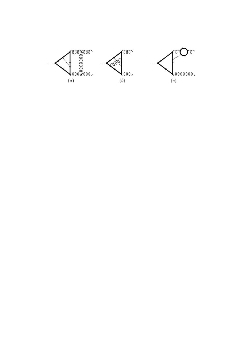
FIG. 1.: Feynman diagrams contribution to the coefficient function $C_{1}$. The internal dashed line either represents the Higgs boson ($h$) or the neutral ($\chi$) or charged ($\phi^{\pm}$) Goldstone boson. The external dashed line corresponds to the Higgs boson.

III Renormalization group functions up to ${\cal O}(\alpha_{s}^{2}x_{t})$

In this section the renormalization constants for different parameters and fields of the QCD Lagrangian are computed in the $\overline{\rm MS}$ scheme using dimensional regularization. Besides QCD corrections also the leading electroweak terms proportional to $m_{t}^{2}$ are taken into account. Thus, in principle an index “$(6)$” indicating the number of active flavours would be necessary which is, however, omitted in this section. As only pole parts in $D-4$ have to be evaluated it is possible to reduce the calculation to massless propagator type diagrams, where the scale is given by the external momentum. In the case of pure QCD such a strategy is common practice, but also for the corrections of ${\cal O}(x_{t})$ this procedure is applicable. Even in the presence of a heavy top quark the needful factors of $m_{t}$ either arise form the coupling of the scalar particles to the top quark or from the expansion of the internal top quark propagators at most up to linear order.

The definition of the renormalization constants is given in Eqs. (2) and (4). In the following the computation of $Z_{3}$, $\tilde{Z}_{3}$, $\tilde{Z}_{1}$, $Z_{2_{q}}^{L/R}$ and $Z_{m_{q}}$ is presented. The renormalization constants both for the quark-gluon, the three- and four-gluon vertex can be obtained by the use of Slavnov-Taylor identities which relate them to the above five constants [24]:

$$Z_{1}\,\,=\,\,\frac{Z_{3}\tilde{Z}_{1}}{\tilde{Z}_{3}}\,,\qquad Z_{1F_{q}}\,\,=\,\,\frac{Z_{2_{q}}\tilde{Z}_{1}}{\tilde{Z}_{3}}\,,\qquad Z_{4}\,\,=\,\,\frac{Z_{3}\tilde{Z}_{1}^{2}}{\tilde{Z}_{3}^{2}}\,.$$ (21)

For convenience we list in the following also the pure QCD results up to order $\alpha_{s}^{2}$. They were first obtained in [25]. Note that from the results for the renormalization constants the corresponding anomalous dimensions can be computed.

From Eqs. (4) it can be seen that for the computation of $Z_{3}$ corrections to the gluon propagator have to be considered. Some sample diagrams contributing at ${\cal O}(\alpha_{s}^{2}x_{t})$ are pictured in Fig. 2 where the dashed lines represents either the $h$, $\chi$ or $\phi^{\pm}$ boson. The electroweak corrections arise for the first time at two loops. At three-loop order already $224$ diagrams contribute. $Z_{3}$ is obtained from the recursive solution of the equation

$$Z_{3} = 1-K_{\varepsilon}\left(\Pi_{G}(q^{2})Z_{3}\right)\,,$$ (22)

where $\Pi_{G}$ is the transversal part of the gluon polarization function defined through

$$\Pi_{G}^{\mu\nu}(q) = \left(-g^{\mu\nu}q^{2}+q^{\mu}q^{\nu}\right)\Pi_{G}(q^{2})\,.$$ (23)

The operator $K_{\varepsilon}$ extracts the pole parts in $\varepsilon$.

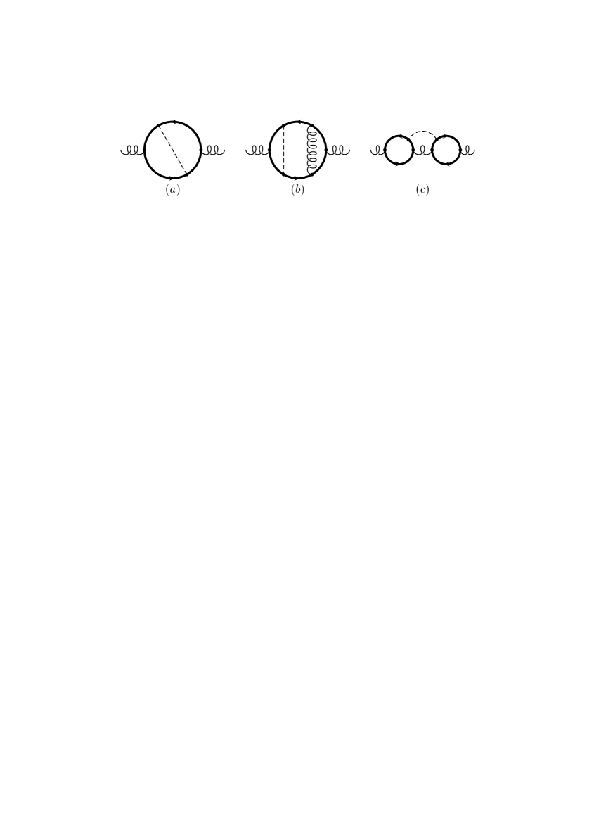
FIG. 2.: Feynman diagrams contribution to $Z_{3}$ and $\zeta_{g}^{0}$. The dashed line either represents the Higgs boson ($h$) or the neutral ($\chi$) or charged ($\phi^{\pm}$) Goldstone boson.

After projecting out $\Pi_{G}(q^{2})$ one ends up with purely massless diagrams. In this case no expansion in $m_{t}$ is required as the factor $m_{t}^{2}$ is provided by the coupling of the scalar bosons to the top quark. For the generation of the diagrams QGRAF [26] is used. The output is then transformed to the package MINCER [27] which is written in FORM [28] and can deal with one-, two- and three-loop massless diagrams with one external momentum different from zero, so-called propagator-type diagrams. After the renormalization of the parameters $\alpha_{s},m_{t}$ and $\xi$ is performed for which only renormalization constants of lower order are needed Eq. (22) has to be solved recursively and one gets

$$Z_{3} = 1+\frac{\alpha_{s}^{(6)}}{\pi}\frac{1}{\varepsilon}\left[C_{A}\,\left(\frac{5}{12}+\frac{1}{8}\xi\right)-T\left(n_{l}+1\right)\frac{1}{3}+x_{t}\,T\right]+\left(\frac{\alpha_{s}^{(6)}}{\pi}\right)^{2}\Bigg{\{}$$ (27)

$$\mbox{}\frac{1}{\varepsilon^{2}}\left[C_{A}^{2}\,\left(-\frac{25}{192}+\frac{5}{384}\xi+\frac{1}{64}\xi^{2}\right)+C_{A}T\left(n_{l}+1\right)\left(\frac{5}{48}-\frac{1}{24}\xi\right)\right]$$

$$\mbox{}+\frac{1}{\varepsilon}\left[C_{A}^{2}\,\left(\frac{23}{128}+\frac{15}{256}\xi-\frac{1}{128}\xi^{2}\right)-C_{F}T\left(n_{l}+1\right)\frac{1}{8}-C_{A}T\left(n_{l}+1\right)\frac{5}{32}\right]$$

$$\mbox{}+x_{t}\,T\left[\frac{1}{\varepsilon^{2}}\left(-C_{F}\frac{1}{2}+C_{A}\left(-\frac{1}{4}+\frac{1}{8}\xi\right)\right)+\frac{1}{\varepsilon}\left(C_{F}\frac{1}{4}+C_{A}\frac{25}{48}\right)\right]\Bigg{\}}\,,$$

where $\alpha_{s}^{(6)}=\alpha_{s}^{(6)}(\mu)$. The superscript “(6)” indicates the number of active flavours. $C_{A}=N_{c}$ and $C_{F}=(N_{c}^{2}-1)/(2N_{c})$ are the Casimir operators of the adjoint and fundamental representation, respectively, and $T=1/2$ is the trace normalization of the fundamental representation. $n_{l}=n_{f}-1=5$ is the number of light (massless) quark flavours.

Special care has to be taken for the diagram pictured in Fig. 2($c$). If the dashed line corresponds to the $\chi$ boson in each fermion line exactly one $\gamma_{5}$ matrix shows up and the naive treatment would fail. In turns out that the diagram is finite and thus gives no contribution to $Z_{3}$. In the next section, however, an analogue diagram contributes to $\zeta_{g}^{0}$ and a careful treatment is mandatory.

In analogy to Eq. (22) the renormalization constant for the ghost field is obtained form

$$\tilde{Z}_{3} = 1-K_{\varepsilon}\left(\Pi_{c}(q^{2})\tilde{Z}_{3}\right)\,.$$ (28)

Corrections of order $x_{t}$ arise for the first time at three-loop level. The result reads:

$$\tilde{Z}_{3} = 1+\frac{\alpha_{s}^{(6)}}{\pi}\frac{1}{\varepsilon}\,C_{A}\,\left(\frac{1}{8}+\frac{1}{16}\xi\right)+\left(\frac{\alpha_{s}^{(6)}}{\pi}\right)^{2}\Bigg{\{}\frac{1}{\varepsilon^{2}}\left[C_{A}^{2}\,\left(-\frac{1}{16}-\frac{3}{256}\xi+\frac{3}{512}\xi^{2}\right)\right.$$ (31)

$$\left.\mbox{}+C_{A}T\left(n_{l}+1\right)\frac{1}{32}\right]+\frac{1}{\varepsilon}\left[C_{A}^{2}\,\left(\frac{49}{768}-\frac{1}{512}\xi\right)-C_{A}T\left(n_{l}+1\right)\frac{5}{192}\right]$$

$$\mbox{}+x_{t}\,C_{A}T\,\left[-\frac{1}{8\varepsilon^{2}}+\frac{23}{96\varepsilon}\right]\Bigg{\}}\,.$$

The renormalization constant $\tilde{Z}_{1}$ requires the computation of gluon-ghost vertex diagrams, $\Gamma_{G\bar{c}c}(q,p)$. For simplicity we choose the gluon momentum to be zero and again end up with massless propagator-type integrals. This could in principle introduce unwanted infrared divergences. However, in [29] it was shown that this is not the case and thus $\tilde{Z}_{1}$ can be computed with the help of the formula

$$\tilde{Z}_{1} = 1-K_{\varepsilon}\left(\Gamma_{G\bar{c}c}(q,0)\tilde{Z}_{1}\right)\,.$$ (32)

Also for $\tilde{Z}_{1}$ the $x_{t}$ corrections in principle appear for the first time at three-loop order. A closer look to the two-loop result shows, however, that those diagrams containing a closed fermion loop add up to zero. As the ${\cal O}(\alpha_{s}^{2}x_{t})$ terms come from the diagrams which contain a top quark loop accompanied with an additional exchange of a scalar particle we expect that $\tilde{Z}_{1}$ gets no ${\cal O}(\alpha_{s}^{2}x_{t})$ corrections at all. This is verified by an explicit calculation. For convenience we list the pure QCD result as it is needed for the computation of $Z_{g}$:

$$\tilde{Z}_{1} = 1+\frac{\alpha_{s}^{(6)}}{\pi}\frac{1}{\varepsilon}\,C_{A}\,\left(-\frac{1}{8}+\frac{1}{8}\xi\right)+\left(\frac{\alpha_{s}^{(6)}}{\pi}\right)^{2}\,C_{A}^{2}\,\Bigg{\{}\frac{1}{\varepsilon^{2}}\left(\frac{5}{128}-\frac{7}{128}\xi+\frac{1}{64}\xi^{2}\right)$$ (34)

$$\mbox{}+\frac{1}{\varepsilon}\left(-\frac{3}{128}+\frac{7}{256}\xi-\frac{1}{256}\xi^{2}\right)\Bigg{\}}\,.$$

The charge renormalization constant, $Z_{g}$, can be computed from the combination of $Z_{3},\tilde{Z}_{3}$ and $\tilde{Z}_{1}$ with the result

$$Z_{g} = \frac{\tilde{Z}_{1}}{\tilde{Z}_{3}\sqrt{Z_{3}}}$$ (35)

$$= 1+\frac{\alpha_{s}^{(6)}}{\pi}\frac{1}{\varepsilon}\left[-C_{A}\frac{11}{24}+T\left(n_{l}+1\right)\frac{1}{6}-x_{t}\,T\frac{1}{2}\right]+\left(\frac{\alpha_{s}^{(6)}}{\pi}\right)^{2}\Bigg{\{}$$ (39)

$$\mbox{}\frac{1}{\varepsilon^{2}}\left[C_{A}^{2}\frac{121}{384}-C_{A}T\left(n_{l}+1\right)\frac{11}{48}+T^{2}\left(n_{l}+1\right)^{2}\frac{1}{24}\right]$$

$$\mbox{}+\frac{1}{\varepsilon}\left[-C_{A}^{2}\frac{17}{96}+C_{A}T\left(n_{l}+1\right)\frac{5}{48}+C_{F}T\left(n_{l}+1\right)\frac{1}{16}\right]$$

$$\mbox{}+x_{t}\,T\left[\frac{1}{\varepsilon^{2}}\left(C_{A}\frac{11}{16}+C_{F}\frac{1}{4}-T\left(n_{l}+1\right)\frac{1}{4}\right)+\frac{1}{\varepsilon}\left(-C_{A}\frac{1}{2}-C_{F}\frac{1}{8}\right)\right]\Bigg{\}}\,.$$

As expected the $\xi$ dependence drops out which is an important check of the calculation.

From the fermion propagator the wave function renormalization constants $Z^{L/R}_{2_{q}}$ and the one for the mass, $Z_{m_{q}}$, can be computed. Due to the different coupling of the $\chi$ boson to up- and down-type quarks, one gets an explicit dependence on the considered quark flavour which is indicated by an additional index. Although in Section IV only $Z_{m_{q}}$ for light quarks is needed we consider for completeness also $Z_{m_{t}}$ as the basic technique of the computation is very similar. The quark two-point function consists of three parts

$$\Sigma(p) = {\not\!p}\left[\Sigma_{V}(p^{2})+\gamma_{5}\Sigma_{A}(p^{2})\right]+m_{q}\Sigma_{S}(p^{2})\,,$$ (40)

where $\Sigma_{V}(p^{2})$ and $\Sigma_{A}(p^{2})$ correspond to the vector and axial-vector and $\Sigma_{S}(p^{2})$ to the scalar part. Note that in the Standard Model the pseudo-scalar contribution to $\Sigma(p)$ is zero. The renormalized fermion propagator can then be written as [30]

$$S_{F}^{-1}(p) = {\not\!p}\left[\frac{1-\gamma_{5}}{2}Z_{2_{q}}^{L}\left(1+\Sigma_{L}(p^{2})\right)+\frac{1+\gamma_{5}}{2}Z_{2_{q}}^{R}\left(1+\Sigma_{R}(p^{2})\right)\right]$$ (42)

$$\quad-m_{q}\sqrt{Z^{L}_{2_{q}}Z^{R}_{2_{q}}}Z_{m_{q}}\left(1-\Sigma_{S}(p^{2})\right)\,,$$

where $\Sigma_{L}(p^{2})$ and $\Sigma_{R}(p^{2})$ are given by

$$\Sigma_{L}(p^{2})\,\,=\,\,\Sigma_{V}(p^{2})-\Sigma_{A}(p^{2})\,,\qquad\Sigma_{R}(p^{2})\,\,=\,\,\Sigma_{V}(p^{2})+\Sigma_{A}(p^{2})\,.$$ (43)

From Eq. (42) the following equations can be derived:

$$Z^{L}_{2_{q}} = 1-K_{\varepsilon}\left(\Sigma_{L}(p^{2})Z^{L}_{2_{q}}\right)\,,$$ (44)

$$Z^{R}_{2_{q}} = 1-K_{\varepsilon}\left(\Sigma_{R}(p^{2})Z^{R}_{2_{q}}\right)\,,$$ (45)

$$\sqrt{Z^{L}_{2_{q}}Z^{R}_{2_{q}}}Z_{m_{q}} = 1+K_{\varepsilon}\left(\Sigma_{S}(p^{2})\sqrt{Z^{L}_{2_{q}}Z^{R}_{2_{q}}}Z_{m_{q}}\right)\,.$$ (46)

Their recursive solutions determine the wave function and mass renormalization constants.

For the computation of $Z^{L/R}_{2_{q}}$ all masses appearing in the propagators may be set to zero and the factors $m_{t}$ are provided by the Yukawa couplings. In the case of the four light quarks only the diagrams where the gluons couple to the considered quark contribute and therefore the renormalization is left-right symmetric:

$$Z^{L}_{2_{l}} = Z^{R}_{2_{l}}$$ (47)

$$= 1+\frac{\alpha_{s}^{(6)}}{\pi}\frac{1}{\varepsilon}\,C_{F}\,\left(\frac{1}{4}\xi-\frac{1}{4}\right)+\left(\frac{\alpha_{s}^{(6)}}{\pi}\right)^{2}\Bigg{\{}\frac{1}{\varepsilon^{2}}\left[C_{F}^{2}\,\left(\frac{1}{32}-\frac{1}{16}\xi+\frac{1}{32}\xi^{2}\right)\right.$$ (50)

$$\left.\mbox{}+C_{A}C_{F}\,\left(\frac{1}{16}-\frac{5}{64}\xi+\frac{1}{64}\xi^{2}\right)\right]+\frac{1}{\varepsilon}\left[C_{F}^{2}\frac{3}{64}+C_{A}C_{F}\,\left(-\frac{17}{64}\right.\right.$$

$$\left.\left.\mbox{}+\frac{5}{64}\xi-\frac{1}{128}\xi^{2}\right)+C_{F}T\left(n_{l}+1\right)\frac{1}{16}\right]-x_{t}\,C_{F}T\frac{1}{4\varepsilon}\Bigg{\}}\,.$$

Next to the pure QCD corrections the class of diagrams pictured in Fig. 3($b$) give rise to the ${\cal O}(\alpha_{s}^{2}x_{t})$ corrections.

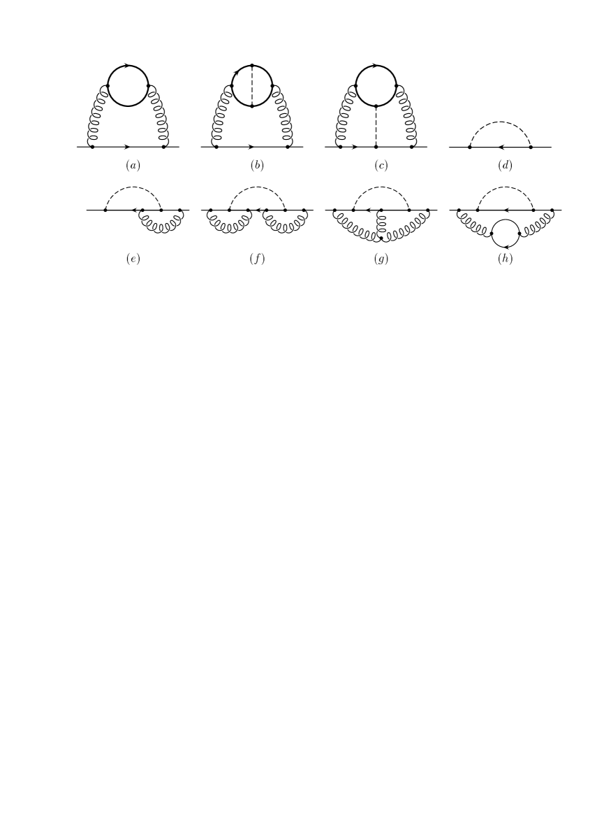
FIG. 3.: Feynman diagrams contribution to $Z_{2_{q}}$, $Z_{m_{q}}$ and $\zeta_{m_{q}}^{0}$. The dashed line either represents the Higgs boson ($h$) or the neutral ($\chi$) or charged ($\phi^{\pm}$) Goldstone boson.

In our approximation the bottom quark is effectively considered to be massless which has the consequence that the bottom-specific corrections only contribute to $Z^{L}_{2_{b}}$:

$$Z^{R}_{2_{b}} = Z^{R}_{2_{l}}\,,$$ (51)

$$Z^{L}_{2_{b}} = Z^{L}_{2_{l}}+x_{t}\Bigg{\{}-\frac{1}{\varepsilon}+\frac{\alpha_{s}^{(6)}}{\pi}\,C_{F}\,\left[\frac{1}{\varepsilon^{2}}\left(1-\frac{1}{4}\xi\right)+\frac{1}{2\varepsilon}\right]+\left(\frac{\alpha_{s}^{(6)}}{\pi}\right)^{2}\Bigg{\{}$$ (56)

$$\mbox{}\frac{1}{\varepsilon^{3}}\left[C_{F}^{2}\,\left(-\frac{19}{32}+\frac{1}{4}\xi-\frac{1}{32}\xi^{2}\right)+C_{A}C_{F}\,\left(-\frac{7}{24}+\frac{5}{64}\xi-\frac{1}{64}\xi^{2}\right)\right.$$

$$\left.\mbox{}+C_{F}T\,\left(n_{l}+1\right)\frac{1}{12}\right]+\frac{1}{\varepsilon^{2}}\left[C_{F}^{2}\,\left(-\frac{23}{64}+\frac{1}{8}\xi\right)+C_{A}C_{F}\,\left(\frac{151}{192}-\frac{5}{64}\xi+\frac{1}{128}\xi^{2}\right)\right.$$

$$\left.\mbox{}-C_{F}T\,\left(n_{l}+1\right)\frac{7}{48}\right]+\frac{1}{\varepsilon}\left[C_{F}^{2}\,\left(\frac{17}{64}-\frac{1}{4}\zeta(3)\right)+C_{A}C_{F}\,\left(-\frac{31}{192}+\frac{5}{8}\zeta(3)\right)\right.$$

$$\left.\mbox{}+C_{F}T\,\left(n_{l}+1\right)\frac{1}{16}\right]\Bigg{\}}\Bigg{\}}\,,$$

with $\zeta(3)\approx 1.202\,057$. For the top quark altogether more diagrams have to be taken into account as — in contrast to the bottom case — already at one- and two-loop level the exchange of a Higgs and neutral Goldstone boson may occur. This is also the reason that both $Z^{L}_{2_{t}}$ and $Z^{R}_{2_{t}}$ get contributions from the top-specific diagrams. We get:

$$Z^{L}_{2_{t}} = Z^{L}_{2_{b}}\,,$$ (57)

and

$$Z^{R}_{2_{t}} = Z^{R}_{2_{l}}+x_{t}\Bigg{\{}-\frac{2}{\varepsilon}+\frac{\alpha_{s}^{(6)}}{\pi}\,C_{F}\,\left[\frac{1}{\varepsilon^{2}}\left(2-\frac{1}{2}\xi\right)+\frac{1}{\varepsilon}\right]+\left(\frac{\alpha_{s}^{(6)}}{\pi}\right)^{2}\Bigg{\{}$$ (61)

$$\mbox{}\frac{1}{\varepsilon^{3}}\left[C_{F}^{2}\,\left(-\frac{19}{16}+\frac{1}{2}\xi-\frac{1}{16}\xi^{2}\right)+C_{A}C_{F}\,\left(-\frac{7}{12}+\frac{5}{32}\xi-\frac{1}{32}\xi^{2}\right)+C_{F}T\,\left(n_{l}+1\right)\frac{1}{6}\right]$$

$$\mbox{}+\frac{1}{\varepsilon^{2}}\left[C_{F}^{2}\,\left(-\frac{23}{32}+\frac{1}{4}\xi\right)+C_{A}C_{F}\,\left(\frac{151}{96}-\frac{5}{32}\xi+\frac{1}{64}\xi^{2}\right)-C_{F}T\,\left(n_{l}+1\right)\frac{7}{24}\right]$$

$$\mbox{}+\frac{1}{\varepsilon}\left[C_{F}^{2}\,\left(\frac{17}{32}-\frac{1}{2}\zeta(3)\right)+C_{A}C_{F}\,\left(-\frac{31}{96}+\frac{5}{4}\zeta(3)\right)+C_{F}T\,\left(n_{l}+1\right)\frac{1}{8}\right]\Bigg{\}}\Bigg{\}}\,.$$

Note that the top-specific corrections of Eq. (61) are exactly twice as large as the ones of Eq. (57).

As can be seen form Eq. (46) the scalar part $\Sigma_{S}$ can be used together with $Z^{L}_{2_{q}}$ and $Z^{R}_{2_{q}}$ in order to compute $Z_{m_{q}}$. For it an expansion of $\Sigma(p)$ in $m_{q}$ up to linear order is necessary in order to be able to project out $\Sigma_{S}$ and end up with massless two-point functions. Notice that here the factor $m_{t}$ may also origin from internal top quark propagators. The class of diagrams pictured in Fig. 3$(c)$ only contributes to $\Sigma_{S}$. Special care has to be taken when the $\chi$ boson is exchanged between the top quark loop and the light fermion line as then each fermion line contains exactly one $\gamma_{5}$. These diagrams, however, only develop an overall divergence giving rise to an simple $1/\varepsilon$ pole. Therefore we are allowed to adopt a prescription for $\gamma_{5}$ according to ’t Hooft and Veltman [31] which was also used in [11] and which is described in more detail in the next section. The result for $q\not=b,t$ reads:

$$Z_{m_{l}} = 1+\frac{\alpha_{s}^{(6)}}{\pi}\frac{1}{\varepsilon}\,C_{F}\left(-\frac{3}{4}\right)+\left(\frac{\alpha_{s}^{(6)}}{\pi}\right)^{2}\Bigg{\{}\frac{1}{\varepsilon^{2}}\left(C_{F}^{2}\frac{9}{32}+C_{A}C_{F}\frac{11}{32}-C_{F}T\left(n_{l}+1\right)\frac{1}{8}\right)$$ (64)

$$\mbox{}+\frac{1}{\varepsilon}\left(-C_{F}^{2}\frac{3}{64}-C_{A}C_{F}\frac{97}{192}+C_{F}T\left(n_{l}+1\right)\frac{5}{48}\right)$$

$$\mbox{}+x_{t}\,C_{F}T\left[\frac{1}{2\varepsilon^{2}}+\frac{1}{\varepsilon}\left(\frac{13}{24}-3\zeta(3)+2I_{3l}\left(\frac{1}{2}+3\zeta(3)\right)\right)\right]\Bigg{\}}\,.$$

The ${\cal O}(\alpha_{s}^{2}x_{t})$ corrections arise from the diagrams shown in Fig. 3$(b)$ and $(c)$. $I_{3l}$ is the third component of the weak isospin, i.e. $I_{3l}=+1/2$ for up-type quarks and $I_{3l}=-1/2$ for down-type quark flavours. The case of the bottom quark exhibits more structures and gives the result

$$Z_{m_{b}} = Z_{m_{d}}+x_{t}\Bigg{\{}-\frac{3}{2\varepsilon}+\frac{\alpha_{s}^{(6)}}{\pi}\,C_{F}\,\left[\frac{9}{4\varepsilon^{2}}-\frac{3}{2\varepsilon}\right]+\left(\frac{\alpha_{s}^{(6)}}{\pi}\right)^{2}\Bigg{\{}$$ (68)

$$\mbox{}\frac{1}{\varepsilon^{3}}\left[-C_{F}^{2}\frac{117}{64}-C_{A}C_{F}\frac{55}{64}+C_{F}T\left(n_{l}+1\right)\frac{5}{16}\right]+\frac{1}{\varepsilon^{2}}\left(C_{F}^{2}\frac{261}{128}+C_{A}C_{F}\frac{285}{128}\right.$$

$$\mbox{}\left.-C_{F}T\left(n_{l}+1\right)\frac{17}{32}\right)+\frac{1}{\varepsilon}\left(C_{F}^{2}\,\left(-\frac{61}{128}+\frac{33}{8}\zeta(3)\right)+C_{A}C_{F}\,\left(-\frac{805}{384}-\frac{15}{16}\zeta(3)\right)\right.$$

$$\mbox{}\left.+C_{F}T\,\left(n_{l}+1\right)\frac{41}{96}\right)\Bigg{\}}\Bigg{\}}\,.$$

Finally for the case of the top quark we obtain

$$Z_{m_{t}} = Z_{m_{u}}+x_{t}\Bigg{\{}\frac{3}{2\varepsilon}+\frac{\alpha_{s}^{(6)}}{\pi}\,C_{F}\,\left[-\frac{9}{4\varepsilon^{2}}+\frac{3}{2\varepsilon}\right]+\left(\frac{\alpha_{s}^{(6)}}{\pi}\right)^{2}\Bigg{\{}$$ (72)

$$\mbox{}\frac{1}{\varepsilon^{3}}\left[C_{F}^{2}\frac{117}{64}+C_{A}C_{F}\frac{55}{64}-C_{F}T\left(n_{l}+1\right)\frac{5}{16}\right]+\frac{1}{\varepsilon^{2}}\left(-C_{F}^{2}\frac{261}{128}-C_{A}C_{F}\frac{285}{128}\right.$$

$$\mbox{}\left.+C_{F}T\left(n_{l}+1\right)\frac{17}{32}\right)+\frac{1}{\varepsilon}\left(C_{F}^{2}\,\left(\frac{157}{128}-\frac{9}{8}\zeta(3)\right)+C_{A}C_{F}\,\left(\frac{239}{128}-\frac{9}{16}\zeta(3)\right)\right.$$

$$\mbox{}\left.-C_{F}T\,\left(n_{l}+1\right)\frac{11}{32}\right)\Bigg{\}}\Bigg{\}}\,.$$

It is remarkable that except for the $1/\varepsilon$ pole at ${\cal O}(\alpha_{s}^{2}x_{t})$ the coefficients of the structures $x_{t}(\alpha_{s}^{(6)}/\pi)^{n}/\varepsilon^{m}$ coincide in the expressions for $Z_{m_{b}}$ and $Z_{m_{t}}$ up to an overall sign.

IV Decoupling relations

The computation of the decoupling constant relating $\alpha_{s}$ in the full and the effective theory requires essentially three ingredients: the hard part of the gluon polarization function, the one for the ghost polarization function and the one of the ghost-gluon vertex. At the one-loop order altogether only one diagram contributes to $\Pi_{G}^{0h}$, namely the one containing a closed top quark loop which is obviously gauge invariant. This is also the case for the ${\cal O}(\alpha_{s}x_{t})$ result where inside the top loop an additional scalar particle is exchanged. At two-loop level $\Pi_{c}^{0h}$ and $\Gamma_{G\bar{c}c}^{0h}$ only receive pure QCD contributions. Actually, the individual diagrams contributing to $\Gamma_{G\bar{c}c}^{0h}$ give non-vanishing contributions, the sum, however, adds up to zero. At three-loop level there are 224, 14, respectively, 98 diagrams which have to be taken into account in order to compute of $\Pi_{G}^{0h}$, $\Pi_{c}^{0h}$, respectively, $\Gamma_{G\bar{c}c}^{0h}$ up to order $\alpha_{s}^{2}x_{t}$. Again, the separate diagrams contributing to $\Gamma_{G\bar{c}c}^{0h}$ add up to zero. $\Pi_{c}^{0h}$ gets non-vanishing corrections which have to be combined with $\Pi_{G}^{0h}$. For the generation of the diagrams the program QGRAF [26] is used. The output is then transformed into a format suitable for the package MATAD [32] which is written in FORM [28] for the purpose to compute one-, two- and three-loop tadpole diagrams.

A special treatment is necessary for the class of diagrams pictured in Fig. 2($c$) where the dashed line represents the neutral CP odd Goldstone boson, $\chi$. Here, $\gamma^{5}$ occurs in two different fermion lines and the naive treatment would lead to a wrong result. Instead we follow the work of ’t Hooft and Veltman [31] and write $\gamma^{5}$ in the form

$$\gamma^{5} = \frac{i}{4!}\epsilon_{\mu\nu\rho\sigma}\gamma^{[\mu\nu\rho\sigma]}\,,$$ (73)

where $\gamma^{[\mu\nu\rho\sigma]}$ is the anti-symmetrized product of four $\gamma$ matrices. The $\epsilon$ tensor is pulled off from the analytical expression and an object containing eight indices is obtained:

$$\Pi^{\mu^{\prime}\nu^{\prime}\rho^{\prime}\sigma^{\prime}}_{G,\mu\nu\rho\sigma}(q^{2}) = \Pi_{G,1}(q^{2})q^{2}g_{[\mu}^{[\mu^{\prime}}g_{\nu}^{\nu^{\prime}}g_{\rho}^{\rho^{\prime}}g_{\sigma]}^{\sigma^{\prime}]}+\Pi_{G,2}(q^{2})q_{[\mu}q^{[\mu^{\prime}}g_{\nu}^{\nu^{\prime}}g_{\rho}^{\rho^{\prime}}g_{\sigma]}^{\sigma^{\prime}]}\,.$$ (74)

$\Pi_{G,1}$ and $\Pi_{G,2}$ are functions of $q^{2}$ and may be extracted with the help of the projectors [33]:

$$P_{1,\mu\nu\rho\sigma}^{\mu^{\prime}\nu^{\prime}\rho^{\prime}\sigma^{\prime}}(q) = \frac{24}{(q^{2})^{2}}\,\frac{\left(q^{2}g_{[\mu}^{[\mu^{\prime}}g_{\nu}^{\nu^{\prime}}g_{\rho}^{\rho^{\prime}}g_{\sigma]}^{\sigma^{\prime}]}-4q_{[\mu}q^{[\mu^{\prime}}g_{\nu}^{\nu^{\prime}}g_{\rho}^{\rho^{\prime}}g_{\sigma]}^{\sigma^{\prime}]}\right)}{(D-1)(D-2)(D-3)(D-4)}\,,$$ (75)

$$P_{2,\mu\nu\rho\sigma}^{\mu^{\prime}\nu^{\prime}\rho^{\prime}\sigma^{\prime}}(q) = \frac{96}{(q^{2})^{2}}\,\frac{\left(-q^{2}g_{[\mu}^{[\mu^{\prime}}g_{\nu}^{\nu^{\prime}}g_{\rho}^{\rho^{\prime}}g_{\sigma]}^{\sigma^{\prime}]}+Dq_{[\mu}q^{[\mu^{\prime}}g_{\nu}^{\nu^{\prime}}g_{\rho}^{\rho^{\prime}}g_{\sigma]}^{\sigma^{\prime}]}\right)}{(D-1)(D-2)(D-3)(D-4)}\,.$$ (76)

Note that both $P_{1}$ and $P_{2}$ develop a $1/\varepsilon$ pole which is a consequence of the fact that for $D=4$ both structures appearing in Eq. (74) are linear dependent. This artificial pole, however, cancels in each diagram individually leading to a finite result. This was actually expected as there is no contribution to $Z_{g}$ from this class of diagrams at the order considered in this paper.

Some comments concerning the renormalization are in order. The parameters in the lower order diagrams have to be replaced by the corresponding renormalized values. Concerning pure QCD, the counterterms for $\alpha_{s}$ and $m_{t}$ have to be known up to order $\alpha_{s}x_{t}$. In principle also the QCD gauge parameter $\xi$ appears in the individual contributions $\Pi_{G}^{0h}$, $\Pi_{c}^{0h}$ and $\Gamma_{G\bar{c}c}^{0h}$, however, only starting from three loops, which has no effect on the terms of order $\alpha_{s}^{2}x_{t}$. The parameters which are present in the diagrams contributing to the ${\cal O}(\alpha_{s}x_{t})$ results receive only contributions from pure QCD counterterms.

In order to compute the renormalized quantity $\zeta_{g}$ also the renormalization constants $Z_{g}^{(5)}$ and $Z_{g}^{(6)}$ are needed. We choose to express the r.h.s. of Eq. (6) in terms of $\alpha_{s}^{(6)}$. Therefore $Z_{g}^{(5)}$ gets a dependence on $m_{t}$ through the substitution of $\alpha_{s}^{(5)}$ whereas before only pure QCD terms were present. $Z_{g}^{(6)}$ has to be known up to order $\alpha_{s}^{2}x_{t}$ which was derived in the previous section. Finally we obtain for $\zeta_{g}$ the following result:

$$\zeta_{g}^{2} = 1+\frac{\alpha_{s}^{(6)}(\mu)}{\pi}\,T\,\Bigg{\{}-\frac{1}{3}\ln\frac{\mu^{2}}{m_{t}^{2}}+\frac{\alpha_{s}^{(6)}(\mu)}{\pi}\left[C_{F}\,\left(-\frac{13}{48}+\frac{1}{4}\ln\frac{\mu^{2}}{m_{t}^{2}}\right)\right.$$ (81)

$$\left.\mbox{}+C_{A}\,\left(\frac{2}{9}-\frac{5}{12}\ln\frac{\mu^{2}}{m_{t}^{2}}\right)+T\,\frac{1}{9}\ln^{2}\frac{\mu^{2}}{m_{t}^{2}}\right]+x_{t}\Bigg{\{}-\frac{2}{3}+\ln\frac{\mu^{2}}{m_{t}^{2}}$$

$$\mbox{}+\frac{\alpha_{s}^{(6)}(\mu)}{\pi}\left[C_{F}\,\left(-\frac{17}{16}+\frac{5}{4}\zeta(2)+\frac{25}{8}\zeta(3)-3\ln\frac{\mu^{2}}{m_{t}^{2}}+\frac{3}{4}\ln^{2}\frac{\mu^{2}}{m_{t}^{2}}\right)\right.$$

$$\left.\mbox{}+C_{A}\,\left(-\frac{5}{4}+\frac{3}{8}\zeta(2)-\frac{95}{64}\zeta(3)+\frac{7}{4}\ln\frac{\mu^{2}}{m_{t}^{2}}\right)+T\,\left(\frac{5}{4}+\frac{7}{8}\zeta(3)+\frac{4}{9}\ln\frac{\mu^{2}}{m_{t}^{2}}\right.\right.$$

$$\left.\left.\mbox{}-\frac{2}{3}\ln^{2}\frac{\mu^{2}}{m_{t}^{2}}\right)-\frac{7}{2}\zeta(3)T\right]\Bigg{\}}\Bigg{\}}\,,$$

where the contribution of the diagrams in Fig. 2($c$) corresponds to the last entry in the last line of Eq. (81). For convenience also the pure QCD result of ${\cal O}(\alpha_{s}^{2})$ is listed. The corresponding three-loop terms can be found in [34, 17].

The decoupling constants for the light masses, $\zeta_{m_{q}}$, requires the computation of the hard part of the fermion propagator. Implicitly this has already been done in [11] where, however, the main focus was on the evaluation of $C_{2_{q}}$, the effective coupling to light quarks. In this paper we will also list the result for $\zeta_{m_{q}}$. As already mentioned above $\zeta_{m_{q}}$ depends on the considered quark flavour which can be seen by a look to the diagrams pictured in Fig. 3. Some words are in order in connections with the diagram in Fig. 3$(c)$ when the dashed line corresponds to the $\chi$ boson. Actually this diagram is responsible for the difference between $\zeta_{m_{u}}$ and $\zeta_{m_{d}}$, as the $\chi\bar{f}f$ coupling is proportional to the third component of the isospin. Furthermore, the treatment of $\gamma_{5}$ needs some care. As already mentioned in Section III the diagrams of this class have an overall divergence which is reflected in the $1/\varepsilon$ pole contributing to $Z_{m_{q}}$ whereas all subdiagrams are finite. Thus we are allowed to adopt the prescription for $\gamma_{5}$ described above. The decoupling constant for the $u,d,s$ and $c$ quark then reads (for simplicity we set $N_{c}=3$):

$$\zeta_{m_{l}} = 1+\left(\frac{\alpha_{s}^{(6)}(\mu)}{\pi}\right)^{2}\Bigg{\{}\frac{89}{432}-\frac{5}{36}\ln\frac{\mu^{2}}{m_{t}^{2}}+\frac{1}{12}\ln^{2}\frac{\mu^{2}}{m_{t}^{2}}$$ (84)

$$\mbox{}+x_{t}\left[\frac{101}{144}-\frac{5}{12}\zeta(2)+\frac{73}{12}\zeta(3)-9\zeta(4)-\frac{7}{6}\ln\frac{\mu^{2}}{m_{t}^{2}}+6\zeta(3)\ln\frac{\mu^{2}}{m_{t}^{2}}\right.$$

$$\mbox{}\left.+2I_{3l}\left(-\frac{37}{18}-\frac{19}{3}\zeta(3)+9\zeta(4)-\ln\frac{\mu^{2}}{m_{t}^{2}}-6\zeta(3)\ln\frac{\mu^{2}}{m_{t}^{2}}\right)\right]\Bigg{\}}\,.$$

For the bottom quark one receives:

$$\zeta_{m_{b}} = \zeta_{m_{d}}+x_{t}\Bigg{\{}\frac{5}{4}+\frac{3}{2}\ln\frac{\mu^{2}}{m_{t}^{2}}+\frac{\alpha_{s}^{(6)}(\mu)}{\pi}\left[\frac{16}{3}-4\zeta(2)+\frac{7}{2}\ln\frac{\mu^{2}}{m_{t}^{2}}+\frac{3}{2}\ln^{2}\frac{\mu^{2}}{m_{t}^{2}}\right]$$ (89)

$$\mbox{}+\left(\frac{\alpha_{s}^{(6)}(\mu)}{\pi}\right)^{2}\left[\frac{472933}{12096}-\frac{6133}{168}\zeta(2)+\frac{905}{72}\zeta(3)+\frac{383}{18}\zeta(4)+\frac{1251}{112}S_{2}+\frac{19}{72}D_{3}\right.$$

$$\mbox{}\left.-\frac{7}{9}B_{4}+\left(\frac{763}{18}-\frac{55}{3}\zeta(2)-\frac{43}{4}\zeta(3)\right)\ln\frac{\mu^{2}}{m_{t}^{2}}+\frac{529}{48}\ln^{2}\frac{\mu^{2}}{m_{t}^{2}}+\frac{29}{12}\ln^{3}\frac{\mu^{2}}{m_{t}^{2}}\right.$$

$$\mbox{}\left.+n_{l}\left(-\frac{23}{24}+\frac{31}{36}\zeta(2)-2\zeta(3)+\left(-\frac{241}{144}+\frac{2}{3}\zeta(2)\right)\ln\frac{\mu^{2}}{m_{t}^{2}}-\frac{1}{2}\ln^{2}\frac{\mu^{2}}{m_{t}^{2}}\right.\right.$$

$$\mbox{}\left.\left.-\frac{1}{12}\ln^{3}\frac{\mu^{2}}{m_{t}^{2}}\right)\right]\Bigg{\}}\,,$$

where we have used $C_{F}=4/3$, $C_{A}=3$ and $T=1/2$. The constants

$$S_{2} = {4\over 9\sqrt{3}}\mbox{Cl}_{2}\left({\pi\over 3}\right)\,\,\approx\,\,0.260\,434\,,$$ (90)

$$D_{3} = 6\zeta(3)-\frac{15}{4}\zeta(4)-6\left(\mbox{Cl}_{2}\left({\pi\over 3}\right)\right)^{2}\,\,\approx\,\,-3.027\,009\,,$$ (91)

$$B_{4} = 16\mathop{{\mbox{Li}}_{4}}\nolimits\left({1\over 2}\right)-{13\over 2}\zeta(4)-4\zeta(2)\ln^{2}2+{2\over 3}\ln^{4}2\,\,\approx\,\,-1.762\,800\,,$$ (92)

where $\zeta(4)=\pi^{4}/90$, $\mbox{Cl}_{2}$ is Clausen’s function and $\mbox{Li}_{4}$ is the quadrilogarithm, occur in the evaluation of the three-loop master diagrams [35, 36, 37]. In [17] the three-loop corrections of ${\cal O}(\alpha_{s}^{3})$ were computed. The results of Eqs. (84) and (89) will be used in the next section in order to compute $C_{2_{l}}$ and $C_{2_{b}}$.

V Hadronic Higgs decay

In this section we compute the coefficient function $C_{1}$ using two different methods. The first one is concerned with the direct evaluation of the triangle diagrams (see Fig. 1) connecting the Higgs boson to two gluons. In a second step $C_{1}$ is evaluated with the help of the LET where the result of the decoupling constant $\zeta_{g}$ derived in the previous section is used.

At three-loop level altogether $990$ diagrams contribute to the order $\alpha_{s}^{2}x_{t}$. Some typical examples are pictured in Fig. 1 where the internal dashed line either represents the Higgs boson, $h$, the neutral Goldstone boson, $\chi$, or the charged Goldstone boson, $\phi^{\pm}$. In the latter case also the bottom quark is present in the fermion loop. The external Higgs boson, however, only couples to top quarks as corrections proportional to $x_{t}$ are considered. The diagrams have to be expanded in both external momenta and the transversal structure which arises from the external gluons is projected out in order to end up with scalar integrals.

Again, the packages QGRAF [26] and MATAD [32] are used for the generation, respectively, the computation of the diagrams. A general gauge parameter, $\xi$, for QCD is used and the independence of the final result serves as a welcome check for the correctness of the result. There is again a class of diagrams which requires a special treatment due to the fact that $\gamma_{5}$ appears in two different fermion lines. A sample diagram is shown in Fig. 1$(c)$. Of course, this class is tightly connected to the one discussed in connection with $\zeta_{g}$ (see Fig. 2$(c)$) and we can adopt the handling for $\gamma_{5}$ developed in Section IV. From Eq. (81) one can see that no $\ln m_{t}$ terms are present which has the consequence that according to the low-energy theorem of Eq. (20) $C_{1}$ gets no contribution from these diagrams. This is confirmed by the direct calculation of the vertex diagrams: there is no contribution from this class of graphs.

After taking into account the counterterms needed to get the renormalized coefficient function (see Eq.(17)) one arrives at:

$$C_{1} = -\frac{1}{6}\,T\,\frac{\alpha_{s}^{(6)}(\mu)}{\pi}\Bigg{\{}1-3x_{t}+\frac{\alpha_{s}^{(6)}(\mu)}{\pi}\left[-C_{F}\,\frac{3}{4}+C_{A}\,\frac{5}{4}-T\,\frac{1}{3}\ln\frac{\mu^{2}}{m_{t}^{2}}\right.$$ (94)

$$\left.\mbox{}+x_{t}\left(C_{F}\,\left(9-\frac{9}{2}\ln\frac{\mu^{2}}{m_{t}^{2}}\right)-C_{A}\,\frac{21}{4}+T\,\left(-\frac{2}{3}+2\ln\frac{\mu^{2}}{m_{t}^{2}}\right)\right)\right]\Bigg{\}}\,.$$

The ${\cal O}(\alpha_{s}x_{t})$ terms can be found in [15] and the ${\cal O}(\alpha_{s}^{2})$ results were computed in [12, 13]. The QCD corrections of ${\cal O}(\alpha_{s}^{3})$ and ${\cal O}(\alpha_{s}^{4})$ are also known [14, 17], however, for simplicity they are not displayed in Eq. (94).

If we use the decoupling constant of Eq. (81) and plug it into Eq. (20) we obtain the identical result which serves as a non-trivial check. Note that the diagrams to be considered in both approaches are quite different. Furthermore, the method based on the LET requires the renormalization constant $Z_{g}$ to be known at ${\cal O}(\alpha_{s}^{2}x_{t})$ whereas for the direct computation only the terms up to order $\alpha_{s}x_{t}$ are necessary.

For completeness we also list the result for $C_{2_{q}}$ obtained from Eqs. (84), respectively, (89) and Eq. (20). For the light quarks we get

$$C_{2_{l}} = 1+\left(\frac{\alpha_{s}^{(6)}(\mu)}{\pi}\right)^{2}\left[\frac{5}{18}-\frac{1}{3}\ln\frac{\mu^{2}}{m_{t}^{2}}+x_{t}\left(\frac{7}{3}-12\zeta(3)+2I_{3l}\left(2+12\zeta(3)\right)\right)\right]\,.$$ (95)

The coefficient function for the bottom quark reads:

$$C_{2_{b}} = C_{2_{d}}+x_{t}\Bigg{\{}-3+\frac{\alpha_{s}^{(6)}(\mu)}{\pi}\left[-7-6\ln\frac{\mu^{2}}{m_{t}^{2}}\right]+\left(\frac{\alpha_{s}^{(6)}(\mu)}{\pi}\right)^{2}\left[-\frac{12169}{144}+\frac{110}{3}\zeta(2)\right.$$ (98)

$$\left.\mbox{}+\frac{43}{2}\zeta(3)-\frac{89}{2}\ln\frac{\mu^{2}}{m_{t}^{2}}-\frac{55}{4}\ln^{2}\frac{\mu^{2}}{m_{t}^{2}}+n_{l}\left(\frac{241}{72}-\frac{4}{3}\zeta(2)+2\ln\frac{\mu^{2}}{m_{t}^{2}}\right.\right.$$

$$\left.\left.\mbox{}+\frac{1}{2}\ln^{2}\frac{\mu^{2}}{m_{t}^{2}}\right)\right]\Bigg{\}}\,.$$

In [11] $C_{2_{l}}$ and $C_{2_{b}}$ are listed for general gauge group $SU(N_{c})$.

Let us now have a look at the numerical consequences on the decay rate. Therefore also the imaginary part of the correlator $\langle[{\cal O}_{1}^{\prime}][{\cal O}_{1}^{\prime}]\rangle$ is needed which can be found in [14]. Furthermore the universal corrections arising from $\bar{\delta}_{u}$ (see Eq. (18)) have to be taken into account. Inserting all building blocks into the equation

$$\Gamma\left(H\to gg\right) = \frac{\sqrt{2}G_{F}}{M_{H}}\left(1+\bar{\delta}_{u}\right)^{2}C_{1}^{2}\,\mbox{Im}\langle[{\cal O}_{1}^{\prime}][{\cal O}_{1}^{\prime}]\rangle$$ (99)

and expanding up to the three-loop level leads to

$$\frac{\Gamma\left(H\to gg\right)}{\Gamma^{\rm Born}(H\to gg)} = 1+x_{t}+\frac{\alpha_{s}^{(5)}(M_{H})}{\pi}\left[23.750-1.667n_{l}\right.$$ (102)

$$\left.\mbox{}+x_{t}\left(38.837+2.000\ln\frac{M_{H}^{2}}{m_{t}^{2}}-1.167n_{l}\right)\right]+\left(\frac{\alpha_{s}^{(5)}(M_{H})}{\pi}\right)^{2}$$

$$\mbox{}\left[370.196-47.186n_{l}+0.902n_{l}^{2}+\left(2.375+0.667n_{l}\right)\ln\frac{M_{H}^{2}}{m_{t}^{2}}\right]$$

$$= 1+x_{t}+\frac{\alpha_{s}^{(5)}(M_{H})}{\pi}\left[17.917+x_{t}\left(33.004+2.000\ln\frac{M_{H}^{2}}{m_{t}^{2}}\right)\right]$$ (104)

$$\mbox{}+\left(\frac{\alpha_{s}^{(5)}(M_{H})}{\pi}\right)^{2}\left[156.808+5.708\ln\frac{M_{H}^{2}}{m_{t}^{2}}\right]\,,$$

with $\Gamma^{\rm Born}(H\to gg)=G_{F}M_{H}^{3}/36\pi\sqrt{2}\times(\alpha_{s}^{(5)}(M_{H})/\pi)^{2}$. The renormalization scale $\mu^{2}$ is set to $M_{H}^{2}$. The resulting logarithms $\ln M_{H}^{2}/m_{t}^{2}$ are numerically small which makes a resummation not necessary [14, 33]. In a similar way to the leading electroweak corrections [15] also at ${\cal O}(\alpha_{s}x_{t})$ large cancellations between the universal and non-universal terms take place. Actually, the “1” in front of the ${\cal O}(x_{t})$ term is composed of $(7-6)$ and the “33.004” results from $(131.504-98.500)$ where in both cases the first number corresponds to the universal corrections. Choosing $m_{t}=m_{t}(M_{H})=173$ GeV and $M_{H}=100$ GeV leads to

$$\frac{\Gamma\left(H\to gg\right)}{\Gamma^{\rm Born}(H\to gg)} = 1+x_{t}+\frac{\alpha_{s}^{(5)}(M_{H})}{\pi}\left(17.917+30.811x_{t}\right)+150.550\left(\frac{\alpha_{s}^{(5)}(M_{H})}{\pi}\right)^{2}$$ (105)

$$\approx 1+0.0031+0.6559+0.0035+0.2017\,.$$ (106)

If one compares the ${\cal O}(x_{t})$ corrections to the pure QCD terms of the same loop order they are clearly negligible. The three-loop corrections of ${\cal O}(\alpha_{s}x_{t})$ amount roughly $1$ % of order $\alpha_{s}^{2}$ terms. It is, however, interesting to note that they have the same sign and that they are of the same order of magnitude as the two-loop corrections of order $x_{t}$.

VI Conclusions

In this paper the gluonic decay of a scalar Higgs boson in the intermediate mass range is considered. The pure QCD corrections up to ${\cal O}(\alpha_{s}^{4})$ were computed recently [14] and it turned out that they are quite sizeable. On the other hand the leading electroweak corrections are small. The main focus of the present paper was the evaluation of additional QCD corrections to the ${\cal O}(x_{t})$ term. Although the new corrections are small as compared to the QCD terms they are quite sizeable as compared to the leading electroweak corrections. It seems that once QCD is switched on and its full structure is available, i.e., the gluon self-interaction is at work, large corrections can be expected. This is also motivated by the comparison of the leading order QCD corrections to $\Gamma(H\to gg)$ and $\Gamma(H\to\gamma\gamma)$. In the latter case only the Abelian part of the QCD enters and the correction factor only amounts to $1-2$ % [38].

In this paper the top quark is considered to be much heavier than the other quarks and the Higgs boson. However, the generalization of the analysis to any heavy quark which fulfills these conditions is straightforward.

Acknowledgments

I would like to thank K.G. Chetyrkin, P.A. Grassi and B.A. Kniehl for useful discussions and comments.

REFERENCES

• [1] P. McNamara, ICHEP โ€™98, Vancouver, July 1998.
• [2] D. Karlen, ICHEP โ€™98, Vancouver, July 1998.
• [3] B.A. Kniehl, Phys. Rep. 240 (1994) 211.
• [4] M. Spira, Fortsch. Phys. 46 (1998) 203.
• [5] E. Braaten and J.P. Leveille, Phys. Rev. D 22 (1980) 715;
M. Drees and K. Hikasa, Phys. Lett. B 240 (1990) 455; B 262 (1991) 497 (E).
• [6] S.G. Gorishny, A.L. Kataev, S.A. Larin, and L.R. Surguladze, Mod.ย Phys.ย Lett. A 5 (1990) 2703; Phys.ย Rev. D 43 (1991) 1633.
• [7] K.G. Chetyrkin, Phys. Lett. B 390 (1997) 309;
K.G. Chetyrkin and M. Steinhauser, Phys. Lett. B 408 (1997) 320.
• [8] B.A. Kniehl, Nucl. Phys. B 376 (1992) 3;
A. Dabelstein and W. Hollik Z. Phys. C 53 (1992) 507.
• [9] A. Kwiatkowski and M. Steinhauser, Phys. Lett. B 338 (1994) 66; B 342 (1995) 455 (E);
B.A. Kniehl and M. Spira, Nucl. Phys. B 432 (1994) 39.
• [10] B.A. Kniehl and M. Steinhauser, Nucl. Phys. B 454 (1995) 485; Phys. Lett. B 365 (1996) 297.
• [11] K.G. Chetyrkin, B.A. Kniehl and M. Steinhauser, Phys. Rev. Lett. 78 (1997) 594; Nucl. Phys. B 490 (1997) 19.
• [12] T. Inami, T. Kubota and Y. Okada, Z. Phys.ย  C 18 (1983) 69.
• [13] A. Djouadi, M. Spira and P.M. Zerwas, Phys.ย Lett.ย  B 264 (1991) 440.
• [14] K.G. Chetyrkin, B.A. Kniehl and M. Steinhauser, Phys. Rev. Lett. 79 (1997) 353.
• [15] A. Djouadi and P. Gambino, Phys. Rev. Lett. 73 (1994) 2528.
• [16] T. Appelquist and J. Carazzone, Phys.ย Rev.ย  D 11 (1975) 2856.
• [17] K.G. Chetyrkin, B.A. Kniehl and M. Steinhauser, Nucl. Phys. B 510 (1998) 61.
• [18] S. Weinberg, Phys.ย Lett.ย  91 B (1980) 51;
B.A. Ovrut and H.J. Schnitzer, Phys.ย Lett.ย  100 B (1981) 403.
• [19] W. Wetzel, Nucl.ย Phys.ย  B 196 (1982) 259;
W. Bernreuther and W. Wetzel, Nucl.ย Phys.ย  B 197 (1982) 228;
W. Bernreuther, Ann.ย Phys.ย  151 (1983) 127; Z. Phys.ย  C 20 (1983) 331.
• [20] S.A. Larin, T. van Ritbergen and J.A.M. Vermaseren, Nucl.ย Phys.ย  B 438 (1995) 278.
• [21] T. van Ritbergen, J.A.M. Vermaseren and S.A. Larin, Phys.ย Lett. B 400 (1997) 379.
• [22] H. Kluberg-Stern and J.B. Zuber, Phys.ย Rev. D 12 (1975) 467;
N.K. Nielsen, Nucl.ย Phys. B 97 (1975) 527; Nucl.ย Phys. B 120 (1977) 212.
• [23] V.P. Spiridonov, INR Report No.ย Pโ€“0378 (1984).
• [24] T. Muta, Foundations of Quantum Chromodynamics (World Scientific, Singapore, 1987).
• [25] D.R.T Jones, Nucl. Phys. B 75 (1974) 531;
A.A. Vladimirov and O.V. Tarasov, Yad. Fiz. 25 (1977) 1104, Sov. J. Nucl. Phys. 25 (1977) 585;
S.Sh. Egorian and O.V. Tarasov, Teor. Mat. Fiz. 41 (1979) 26; Theor. Math. Phys. 41 (1979) 863;
R. Tarrach, Nucl. Phys. B 183 (1981) 384.
• [26] P. Nogueira, J. Comput.ย Phys.ย  105 (1993) 279.
• [27] S.A. Larin, F.V. Tkachov and J.A.M. Vermaseren, Report No.ย NIKHEFโ€“H/91โ€“18 (September 1991).
• [28] J.A.M. Vermaseren, Symbolic Manipulation with FORM, (Computer Algebra Netherlands, Amsterdam, 1991).
• [29] A.I. Davydychev, P. Osland and O.V. Tarasov, Phys. Rev. D 58 (1998) 036007, hep-ph/9801380.
• [30] see e.g.: R. Kawabe, K.i. Aoki, Z. Hioki, M. Konuma and T. Muta, Prog. Theor. Phys. Suppl. 73 (1982) 1.
• [31] G. โ€™t Hooft and M. Veltman, Nucl. Phys. B 44 (72) 189;
P. Breitenlohner and D. Maison, Comm. Math. Phys. 52 (1977) 11.
• [32] M. Steinhauser, Ph.D. thesis, Karlsruhe University (Shaker Verlag, Aachen, 1996).
• [33] K.G. Chetyrkin, B.A. Kniehl, M. Steinhauser and W.A. Bardeen, Report Nos.ย FERMILAB-PUB-98/126-T, MPI/PhT/98โ€“032, NYU-TH/98/04/02, TTP98-21 and hep-ph/9807241 (June 1998) (Nucl. Phys. B in press).
• [34] K.G. Chetyrkin, B.A. Kniehl and M. Steinhauser, Phys. Rev. Lett. 79 (1997) 2184.
• [35] D.J. Broadhurst, Z. Phys. C 54 (1992) 599.
• [36] L. Avdeev, J. Fleischer, S. Mikhailov, and O. Tarasov, Phys.ย Lett. B 336 (1994) 560; (E) B 349 (1995) 597;
K.G. Chetyrkin, J.H. Kรผhn, and M. Steinhauser, Phys.ย Lett. B 351 (1995) 331.
• [37] D.J. Broadhurst, Report Nos. OUT-4102-72 and hep-th/9803091.
• [38] H. Zheng and D. Wu, Phys.ย Rev. D 42 (1990) 3760;
A. Djouadi, M. Spira, J. van der Bij and P.M. Zerwas, Phys.ย Lett. B 257 (1991) 187;
S. Dawson and R.P. Kauffman, Phys.ย Rev. D 47 (1993) 1264;
A. Djouadi, M. Spira and P.M. Zerwas, Phys.ย Lett. B 311 (1993) 255;
K. Melnikov and O. Yakovlev, Phys.ย Lett. B 312 (1993) 179;
M. Inoue, R. Najima, T. Oka and J. Saito, Mod.ย Phys.ย Lett. A 9 (1994) 1189.