CERN-TH/98-315

hep-ph/9809498

Charge and Colour Breaking Constraints in the MSSM With Non-Universal SUSY Breaking

S. A. Abel^a and C. A. Savoy^b

^aTheory Division, Cern 1211, Geneva 23, Switzerland
^bCEA-SACLAY, Service de Physique Théorique,
F-91191 Gif-sur-Yvette Cedex, France

Abstract

We examine charge/colour breaking along directions in supersymmetric field space which are $F$ and $D$-flat. We catalogue the dangerous directions and include some new ones which have not previously been considered. Analytic expressions for the resulting constraints are provided which are valid for all patterns of supersymmetry breaking. As an example we consider a recently proposed pattern of supersymmetry breaking derived in Horava-Witten $M$-theory, and show that there is no choice of parameters for which the physical vacuum is a global minimum.

CERN-TH/98-315

Supersymmetric models often have charge and/or colour breaking minima which can compete with the physical vacuum [1, 2]. Excluding the regions of parameter space that lead to such minima results in bounds which can be severe. There are a number of reasons why supersymmetry suffers from this kind of metastability. There are many flat directions which are lifted only by our choice of supersymmetry breaking parameters. The higgs scalar which couples to the bottom quark, $H_{1}$, has the same quantum numbers as the leptons. Moreover, the mass-squared parameter of the higgs which couples to the top quark, $H_{2}$, is negative at the weak scale (a requirement of electroweak symmetry breaking and one of the successes of supersymmetry).

The resulting charge and colour breaking bounds can be roughly divided into three kinds.

• $D$-flat directions which develop a minimum due to large trilinear supersymmetry breaking terms. They are important at low scales [1] and are usually referred to as CCB bounds.

• $F$ and $D$ flat directions corresponding to a single gauge invariant. These are important when there are negative mass-squared terms at the GUT scale. One therefore needs to take account of the renormalisation group running, but they can be lifted by non-renormalisable terms in the superpotential. They are often referred to as unbounded from below (UFB) bounds [3].

• $F$ and $D$ flat directions which correspond to a combination of gauge invariants involving $H_{2}$. These can develop a minimum at intermediate scales due to the running $H_{2}$ mass even if all the mass-squareds are positive at the GUT scale. They cannot be lifted by non-renormalisable terms. They are also (rather confusingly) referred to as UFB bounds.

The 3rd kind of bound will be of interest here since they can be very severe. For example, the Constrained MSSM (CMSSM) near its low $\tan\beta$ fixed point has almost half its parameter space excluded by them. Combined with dark matter constraints and experimental bounds, this is sufficient to exclude the model entirely [2]. Unfortunately these bounds are also the most difficult to calculate because the renormalisation group running of the soft supersymmetry breaking parameters plays a complicated role in their determination. Specifically, the dangerous minimum forms where the running (negative) $H_{2}$ mass-squared is offset by the other (positive) mass-squared terms.

Hence most work on UFB bounds is done numerically and the models considered typically have few parameters (such as the CMSSM which has only four). The reason for this is a practical one; to properly sample a parameter space one has to include, say, one low and one high representative of each variable. This becomes progressively more difficult as the dimensionality increases and for the most general MSSM (which has $\sim 100$ parameters) it is clearly impossible. Even if it were possible to sample such a large parameter space, extracting any useful information would be extremely difficult.

However, what does one do if a case of phenomenological interest (the real World for example) requires a less restricted set of parameters than that of the CMSSM? How do the UFB bounds restrict supersymmetry breaking in more general models? While determining this would very difficult numerically, it was shown in Ref.[4] that, by making a few simple approximations, we can make a reasonably accurate analytic approximation. In this letter we shall present the analytic expressions for the UFB bounds in the most general supersymmetry breaking scenarios. In particular we will show that there is essentially only one particular combination of supersymmetry breaking parameters which is subject to UFB bounds. This combination is

$$2m^{2}_{L_{ii}}+m_{2}^{2}-m_{U_{33}}^{2}-m_{Q_{33}}^{2},$$ (1)

where the notation for soft supersymmetry breaking parameters is as in Ref.[4].

We begin by ennumerating the dangerous directions, assuming the usual $R$-parity invariant superpotential of the MSSM;

$$W_{MSSM}=h_{U}QH_{2}U^{c}+h_{D}QH_{1}D^{c}+h_{E}LH_{1}E^{c}+\mu H_{1}H_{2}.$$ (2)

As we stated above, the dangerous $F$ and $D$ flat directions are those constructed from gauge invariants involving $H_{2}$ [5, 6]. The first example of this kind in the literature is (see Komatsu in Ref.[1])

$$L_{i}Q_{3}D_{3}\mbox{ ; }H_{2}L_{i}$$ (3)

where the suffices on matter superfields are generation indices. With the following choice of VEVs;

$$h_{2}^{0} = -a^{2}\mu/h_{D_{33}}$$

$$\tilde{d}_{L_{3}}=\tilde{d}_{R_{3}} = a\mu/h_{D_{33}}$$

$$\tilde{\nu}_{i} = a\sqrt{1+a^{2}}\mu/h_{D_{33}},$$ (4)

the potential along this direction is $F$ and $D$-flat, and depends only on the soft supersymmetry breaking terms;

$$V=\frac{\mu^{2}}{h_{D_{33}}^{2}}a^{2}(a^{2}(m_{2}^{2}+m_{L_{ii}}^{2})+m_{L_{ii}}^{2}+m_{d_{33}}^{2}+m_{Q_{33}}^{2}).$$ (5)

This is not quite, but is very close to, the deepest ‘fully optimised’ direction [1]. Two additional points. Note that in this case we can work in the basis in which the relevant Yukawa coupling is diagonal. Also, since the only severe bounds involve the third generation we shall restrict our attention to these cases.

At large values of $a\gg 1$ the potential is governed by the first term. This can be negative at the weak scale because of the negative value of $m_{2}^{2}$. The potential can therefore develop a charge and colour breaking minimum at a scale of $few\times\mu/h_{D_{j}}$ and ensuring that this does not happen leads to the UFB bound.

The coefficients in Eq.(S0.Ex1) were chosen to cancel $F_{H_{1}}=\partial W/\partial{H_{1}}$. However there are other combinations of invariants which can do the same job; in fact $L_{k}H_{2}$ plus any invariant containing either $L_{3}E_{3}$ or $Q_{3}D_{3}$ can cancel $F_{H_{1}}$. However the invariant should not contain $H_{1}$ otherwise $F_{E}$, $F_{D}$, $F_{Q}$ and $F_{L}$ would all be non-zero. The complete basis of gauge invariant monomials in Ref.[6] then tells us that the following invariants are of possible relevance;

$$L_{i}L_{3}E_{3} i\neq 3$$ (6)

$$L_{i}Q_{3}D_{3}$$

$$Q^{\prime}_{i}U_{j}L_{3}E_{3}$$

$$Q^{\prime}_{i}U_{j}Q^{\prime}_{3}D_{3} i\neq 3$$

$$(Q^{\prime}_{1}L_{i})(Q^{\prime}_{2}L_{j})(Q^{\prime}_{3}L_{3})E_{3} +L$$ perms

$$(U_{1}U_{2}D_{i})Q^{\prime}_{3}D_{j}H_{2} \delta_{3i}+\delta_{3j}\neq 0$$

$$(U_{1}U_{2}D_{i})Q^{\prime}_{3}D_{j}Q^{\prime}_{l}D_{m} l\neq 3;\delta_{3i}+\delta_{3j}+\delta_{m3}\neq 0,$$

where groups of three coloured fields are contracted with Levi-Cevita symbols. Note that in the above list, $Q^{\prime}$ is in the up-quark mass basis to ensure that $F_{H_{2}}=0$. The first two directions have already been considered at some length in the literature. However this will be, to our knowledge, the first time that the other directions have been discussed.

We can discard most of the new directions because they have non-zero $F_{Q}$ or $F_{U}$. For example both the $UUDQDH_{2}$ and $UUDQDQD$ directions have non-zero $F_{Q^{\prime}_{2}}$. This is enough to lift the radiative minima since the latter has a depth of $\sim a_{min}^{4}\mu^{2}m_{W}^{2}/h_{b}^{2}$ where $a_{min}={\cal O}(10)$, but

$$F_{Q^{\prime}_{2}}^{2}=h_{c}^{2}a_{min}^{6}\mu^{4}/h_{b}^{4}\gg a_{min}^{4}\mu^{2}m_{W}^{2}/h_{b}^{2}.$$ (7)

Clearly the only dangerous directions involve only the first generation up-quarks. For example, the $Q^{\prime}_{1}U_{1}L_{3}E_{3}$ direction is dangerous. Although it has non-zero $F_{U_{1}}$, $F_{Q^{\prime}_{1}}$ and $F_{H_{2}}$, these $F$-terms are not enough to lift the radiatively induced minima since

$$a_{min}^{2}F^{2}_{H_{2}}=F_{U_{1}}^{2}=F_{Q^{\prime}_{1}}^{2}\approx h_{u}^{2}a_{min}^{6}\mu^{4}/h_{b}^{4}\ll a_{min}^{4}\mu^{2}m_{W}^{2}/h_{b}^{2}.$$ (8)

Similar consideration apply for the $Q^{\prime}UQ^{\prime}D$ direction. Finally the $Q^{\prime}Q^{\prime}Q^{\prime}LLLE$ direction has nothing apart from non-zero $F_{U_{1}}$-terms if we choose VEVs along the $h_{2}^{0}\nu_{k}$ and $U^{\prime}_{L_{1}}D^{\prime}_{L_{2}}D^{\prime}_{L_{3}}E_{L_{3}}\nu_{i}\nu_{j}E_{3}$ directions.

The potentials for these operators (when combined with $h^{0}_{2}\nu_{k}$ and neglecting the small $F^{2}_{U_{1}}$, $F^{2}_{Q^{\prime}_{1}}$ and $F^{2}_{H_{2}}$ terms above) are

$$LLE \rightarrow \frac{\mu^{2}}{h_{E_{33}}^{2}}a^{2}(a^{2}(m_{2}^{2}+m_{L_{kk}}^{2})+\sqrt{a^{2}+1}(1-\delta_{ik})(m^{2}_{L_{ik}}+m^{2}_{L_{ki}})$$

$$\mbox{\hskip 28.45274pt}+m_{L_{ii}}^{2}+m_{L_{33}}^{2}+m_{E_{33}}^{2})$$

$$LQD \rightarrow \frac{\mu^{2}}{h_{D_{33}}^{2}}a^{2}(a^{2}(m_{2}^{2}+m_{L_{kk}}^{2})+\sqrt{a^{2}+1}(1-\delta_{ik})(m^{2}_{L_{ik}}+m^{2}_{L_{ki}})$$

$$\mbox{\hskip 28.45274pt}+m_{L_{ii}}^{2}+m_{Q_{33}}^{2}+m_{D_{33}}^{2})$$

$$QULE \rightarrow \frac{\mu^{2}}{h_{E_{33}}^{2}}a^{2}(a^{2}(m_{2}^{2}+m_{L_{kk}}^{2})+m_{Q^{\prime}_{11}}^{2}+m_{U_{11}}^{2}+m_{L_{33}}^{2}+m_{E_{33}}^{2})$$

$$QUQD \rightarrow \frac{\mu^{2}}{h_{D_{33}}^{2}}a^{2}(a^{2}(m_{2}^{2}+m_{L_{kk}}^{2})+m_{Q^{\prime}_{11}}^{2}+m_{U_{11}}^{2}+m_{Q^{\prime}_{33}}^{2}+m_{D_{33}}^{2})$$

$$QQQLLLE \rightarrow \frac{\mu^{2}}{h_{E_{33}}^{2}}a^{2}(a^{2}(m_{2}^{2}+m_{L_{kk}}^{2})+(1-\delta_{ij})(m_{L_{ij}}^{2}+m_{L_{ji}}^{2})$$ (9)

$$\mbox{\hskip 5.69046pt}+\sqrt{a^{2}+1}(1-\delta_{ij})(m^{2}_{L_{ij}}+m^{2}_{L_{ji}})+\sqrt{a^{2}+1}(1-\delta_{ik})(m^{2}_{L_{ik}}+m^{2}_{L_{ki}})$$

$$+m_{Q_{11}}^{2}+m_{Q_{22}}^{2}+m_{Q_{33}}^{2}+m_{Q_{23}}^{2}+m_{Q_{32}}^{2}+m_{L_{ii}}^{2}+m_{L_{jj}}^{2}+m_{L_{33}}^{2}+m_{E_{33}}^{2})$$

where the $h_{D_{33}}$ should be the Yukawa coupling taken in the up-quark diagonal basis for the $QUQD$ direction. At first glance the last direction seem to be safe because of the large number of mass-squared terms. However, it should be stressed that these parameters are not physical mass-squareds and they can therefore be negative (as is often the case in weakly coupled string models for example). As we shall see however, the renormalisation group running does tend to make them positive towards low scales so that they indeed tend to be less important. The off-diagonal bounds are likely to be unimportant when the relevant mass-squared parameters are positive, so henceforth we shall consider only the diagonal ones.

In order to obtain the UFB bound we now need to take account of the renormalisation group running of the mass-squared parameters between the weak and GUT scales. An accurate analytic method was introduced in Ref.[4] which we shall briefly recap.

First we need to make some approximations and assumptions; they are

• Neglect two loop effects in the renormalization group running of parameters (here we include hypercharge contributions).

• Of the Yukawas, keep only $h_{t}=h_{U_{33}}$ in the runnning – neglect the bottom and tau Yukawas (i.e. $\tan\beta<30$) and mixing.

• Assume that the gaugino masses are degenerate ($M_{3}=M_{2}=M_{1}=M_{1/2}$) at the scale where the gauge couplings unify (which we shall refer to as the GUT scale)

These approximations allow us to obtain analytic solutions for the running parameters in closed form (which were presented in Ref.[4]). In Ref.[4] it was shown that the final analytic expressions for the UFB bounds should be accurate to $\sim 15\%$.

Next, we assume that the largest mass, and therefore the appropriate scale to evaluate the parameters at is $\phi=h_{U_{33}}\langle h_{2}^{0}\rangle$. In the above potentials, $\langle h_{2}^{0}\rangle=-a^{2}\mu/h_{D_{33},E_{33}}$ so that the potentials are of the form

$$V=\frac{M_{GUT}^{2}}{h_{U_{33}}^{2}}\hat{\phi}\left(\hat{\phi}A+B/b\right)$$ (10)

where $A=m_{2}^{2}(\phi)+m_{L_{ii}}^{2}(\phi)$, $B$ is the other combination of mass-squared parameters (also evaluated at $\phi$) which appears in the potentials above,

$$\hat{\phi}=\phi/M_{GUT}$$ (11)

and

$$b(\phi)=\frac{M_{GUT}h_{D_{33}}}{h_{U_{33}}\mu}=\frac{2.9\times 10^{12}}{h_{U_{33}}/1.1}\left(\frac{M_{GUT}}{2\times 10^{16}\,{\rm GeV}}\right)\left(\frac{m_{b}(\phi)}{2.5\,{\rm GeV}}\right)\left(\frac{200\,{\rm GeV}}{\mu(\phi)}\right)$$ (12)

for $h_{D_{33}}$ or

$$b(\phi)=\frac{M_{GUT}h_{E_{33}}}{h_{U_{33}}\mu}=\frac{2.0\times 10^{12}}{h_{U_{33}}/1.1}\left(\frac{M_{GUT}}{2\times 10^{16}\,{\rm GeV}}\right)\left(\frac{m_{\tau}(\phi)}{1.78\,{\rm GeV}}\right)\left(\frac{200\,{\rm GeV}}{\mu(\phi)}\right)$$ (13)

for $h_{E_{33}}$. The traditional UFB bound is saturated by $V=V^{\prime}=0$; the non-trivial solution is therefore also a solution to $\tilde{V}=\tilde{V}^{\prime}=0$ where

$$\tilde{V}=\hat{\phi}A+B/b.$$ (14)

Hence, only the parameter $b$ enters the bound. In fact the bound always becomes more restrictive with increase in $b$, since this decreases the positive contribution to the potential. (The increase with unification scale has already been noted in numerical work, e.g. Casas et al  of Ref.[2].) To solve for the UFB bound we first define the point $\hat{\phi}_{p}$ where

$$A(\phi_{p})=0.$$ (15)

We can then expand about $\phi_{p}$ and solve $\tilde{V}(\phi_{d})={\tilde{V}^{\prime}}(\phi_{d})=0$;

$$\hat{\phi}^{2}_{p} = \left.\frac{eB}{A^{\prime}b}\right|_{\phi_{p}}$$

$$\phi_{d} = e^{-1}\phi_{p}.$$ (16)

Likewise, the sufficient condition is given by, (${\tilde{V}^{\prime\prime}}(\phi_{c})=V^{\prime}(\phi_{c})=0$);

$$\hat{\phi}^{2}_{p} = \left.\frac{e^{3/2}B}{2A^{\prime}b}\right|_{\phi_{p}}$$

$$\phi_{c} = e^{-3/2}\phi_{p}.$$ (17)

The solutions for the running parameters including $b$ and $A^{\prime}$ were given in Ref.[4] in terms of the three parameters with quasi-fixed points;

$$R \equiv h_{U_{33}}^{2}/g_{3}^{2}$$

$$A_{t} \equiv A_{U_{33}}$$

$$3M^{2} \equiv m_{U_{33}}^{2}+m_{Q_{33}}^{2}+m_{2}^{2}.$$ (18)

Using these solutions we can find the value of $\hat{\phi}_{p}$ by solving Eq.(S0.Ex17) or Eq.(S0.Ex18) either numerically or iteratively. Finally we obtain the bound by solving Eq.(15) (which we haven’t yet used);

$$A(\phi_{p})=0=\frac{\mbox{\small 3}}{\mbox{\small 2}}M^{2}+\left.(m_{2}^{2}+m_{L_{ii}}^{2}-\frac{3}{2}M^{2})\right|_{0}-M_{1/2}^{2}(\frac{\mbox{\small 8}}{\mbox{\small 9}}\delta_{3}^{(2)}+\frac{\mbox{\small 3}}{\mbox{\small 2}}\delta_{2}^{(2)}+\frac{\mbox{\small 5}}{\mbox{\small 198}}\delta_{1}^{(2)}),$$ (19)

where

$$\tilde{\alpha}_{i} = \frac{\alpha_{i}}{\alpha_{i}|_{0}}$$

$$\delta_{i}^{(n)} = \tilde{\alpha}^{n}_{i}-1$$ (20)

and the $0$-subscript indicates values at the GUT scale. Using Eqs.(S0.Ex17,19) we are now able to estimate the UFB bounds in any particular case of interest and to get a reasonable estimate for the most general case.

General models at the low $\tan\beta$ fixed point

First consider the low $\tan\beta$ fixed point (where $h_{U_{33}}$ is very large at the GUT scale). As a rule of thumb the UFB constraints are most restrictive here. This is because the dangerous minimum is driven by the negative mass-squared of $H_{2}$ which is in turn driven by the top quark Yukawa coupling. A larger top Yukawa makes $m_{2}^{2}$ negative closer to the GUT scale and the other mass-squared terms have to be larger to overcome it; and the largest possible top Yukawa is at the fixed point.

Here we see why the bounds involve the particular combination appearing in Eq.(1). From Eq.(19) the relevant bound is

$$\left.(m_{2}^{2}+m_{L_{ii}}^{2}-\frac{3}{2}M^{2})\right|_{0}\,\raisebox{-2.58334pt}{$\buildrel>\over{\sim}$}\,\frac{\mbox{\small 3}}{\mbox{\small 2}}M^{2}-M_{1/2}^{2}(\frac{\mbox{\small 8}}{\mbox{\small 9}}\delta_{3}^{(2)}+\frac{\mbox{\small 3}}{\mbox{\small 2}}\delta_{2}^{(2)}+\frac{\mbox{\small 5}}{\mbox{\small 198}}\delta_{1}^{(2)}).$$ (21)

The $M^{2}$ parameter is determined at any particular scale since we are at the fixed point. The only influence the $B/b$ term can have is logarithmic, via the determination of the scale, $\phi_{p}$, at which the RHS should be evaluated. Consider the $LLE$, $LH_{2}$ directions with the central value of $b$. Using the solutions of Ref.[4] this scale is given by

$$\hat{\phi}_{p}=\frac{2\pi e}{3b\alpha|_{0}}\left(\frac{(\tilde{m}_{L_{ii}}^{2}+\tilde{m}_{L_{33}}^{2}+\tilde{m}_{E_{33}}^{2})|_{0}-3\delta_{2}^{(2)}}{\tilde{\alpha}_{3}R(3\tilde{M}^{2}+\tilde{A}_{U_{33}}^{2})-2\tilde{\alpha}_{2}^{3}}\right)$$ (22)

where $\tilde{m}=m/M_{1/2}$, which can be solved iteratively. The final bound is

$$\left.(2\tilde{m}_{L_{ii}}^{2}+\tilde{m}_{2}^{2}-\tilde{m}^{2}_{U_{33}}-\tilde{m}^{2}_{Q_{33}})\right|_{0}\,\raisebox{-2.58334pt}{$\buildrel>\over{\sim}$}\,f(\tilde{B}|_{0})$$ (23)

where

$$\tilde{B}|_{0} = \left.(\tilde{m}_{L_{ii}}^{2}+\tilde{m}_{L_{33}}^{2}+\tilde{m}_{E_{33}}^{2})\right|_{0}$$

$$f(x) \approx 1.43-0.16x+0.02x^{2}.$$ (24)

The last equation is a fit to the bounds which is accurate for $x\,\raisebox{-2.58334pt}{$\buildrel>\over{\sim}$}\,0$. We stress that this result is valid for the MSSM with any pattern of supersymmetry breaking. In the CMSSM, where the scalar masses are degenerate and equal to $m_{0}$ at the GUT scale, the inequality becomes

$$\tilde{m}_{0}^{2}\,\raisebox{-2.58334pt}{$\buildrel>\over{\sim}$}\,f(3\tilde{m}_{0})$$ (25)

and we find the familiar result

$$m_{0}\,\raisebox{-2.58334pt}{$\buildrel>\over{\sim}$}\,1.05M_{1/2}$$ (26)

which is a slight overestimate of the numerical results of Ref.[2] (by $5-10\%$).

We can also examine the dependence on the $b$ parameter for this case. For example, the central value of $b$ had $\mu=200\,{\rm GeV}$. If we take $\mu=500\,{\rm GeV}$ (or $b=7.7\times 10^{11}$) we find

$$f(x)\approx 1.20-0.14x+0.02x^{2}$$ (27)

and for the CMSSM we then find

$$m_{0}\,\raisebox{-2.58334pt}{$\buildrel>\over{\sim}$}\,0.95M_{1/2}.$$ (28)

From this we can conclude that, given the accuracy of our other approximations, there is little point in determining the value of $\mu$ by minimising the potential (which is fortunate since this would have made our task prohibitively difficult). Additionally $M_{GUT}$ is as important as $\mu$ in the determination of the bound and we can reasonably set $\mu=M_{1/2}$ for an estimate of the UFB bound.

Before leaving the fixed point, there is an additional fairly weak bound on $B|_{0}$. When this parameter becomes too negative it is unable to lift the minimum for any GUT scale value of $m^{2}_{L_{ii}}+m_{2}^{2}$. The resulting bound is

$$B|_{0}=\left.(m_{L_{ii}}^{2}+m_{L_{33}}^{2}+m_{E_{33}}^{2})\right|_{0}>-0.7M_{1/2}^{2}.$$ (29)

The values of the functions, $f(x)$, and the above bounds are given in the table for all the directions in Eq.(6). As can be seen the constraints corresponding to the $LLE$, $LH_{2}$ invariants are the strongest. This had been noted before in numerical work on the CMSSM, but here we see it is a completely general result.

$LH_{2}$+Operator	$f(x)$	$g(x)$	$\tilde{B}_{0}\,\raisebox{-2.58334pt}{$\buildrel>\over{\sim}$}\,$
$LLE$	$1.43-0.16x+0.02x^{2}$	$2.94-0.2x+0.02x^{2}$	-0.7
$QDE$	$1.08-0.05x$	$2.55-0.06x$	-3.5
$QULE$	$1.03-0.04x$	$2.49-0.05x$	-4.5
$QUQD$	$0.94-0.02x$	$2.38-0.03x$	-7.2
$QQQLLLE$	$0.96-0.02x$	$2.39-0.03x$	-6.8

General models away from the fixed point

At the fixed point, the bounds do not depend on $M^{2}|_{0}$ or $A_{U_{33}}|_{0}\equiv A_{0}$. As we move away from the fixed point (to higher $\tan\beta$) we find that the dependence on these parameters increases. We now include this dependence. The distance from the fixed point is most conveniently expressed in terms of the parameter

$$\rho=\frac{R}{R^{QFP}}$$ (30)

where $R^{QFP}$ is the fixed point value of $R$ which is simply a function of scale.

The bounds can be evaluated as above from Eq.(19) keeping the dependence on $A_{0}$ and $M^{2}|_{0}$. In order to determine the scale $\phi_{p}$ we can approximate $A^{\prime}(\phi)$ with its fixed point value which is independent of $A_{0}$ and $M^{2}|_{0}$; the actual value is close to the fixed point value even for quite large values of $\tan\beta$ and in any case the scale appears only logarithmically in the determination of the UFB bound. The bounds are found to be

$$\left.(2\tilde{m}_{L_{ii}}^{2}+\tilde{m}_{2}^{2}-\tilde{m}^{2}_{U_{33}}-\tilde{m}^{2}_{Q_{33}})\right|_{0}\,\raisebox{-2.58334pt}{$\buildrel>\over{\sim}$}\,f(\tilde{B}|_{0})+(\rho_{p}-1)\left(g(\tilde{B}|_{0})+3\tilde{M}^{2}|_{0}-\rho_{p}(1-\tilde{A}_{0})^{2}\right),$$ (31)

where $\rho_{p}$ is the value of $\rho$ at the scale $\phi_{p}$. To a very good approximation we find that the value of $\rho_{p}$ is given by [4]

$$\frac{1}{\rho_{p}}=1+\frac{1}{2R_{0}}=1+3.17(\sin^{2}\beta-\sin^{2}\beta^{QFP}),$$ (32)

where $R_{0}$ is the value of $R$ at the GUT scale and $\tan\beta^{QFP}=1.78$ in this approximation (but it should be stressed that the bounds we are evaluating are not dependent on its absolute value but rather the value of $\rho_{p}$). In Eq.(31), $f(x)$ is the bound at the fixed point as before, and $g(x)$ can be approximated in a similar manner. For the $LLE$, $LH_{2}$ direction we find

$$g(x)\approx 2.94-0.20x+0.02x^{2}.$$ (33)

The functions for the remaining directions are given in the table above. We can see that $A_{0}\approx M_{1/2}$ results in the weakest bounds. In addition the bounds asymptote at large $\tan\beta$ to the values with

$$\rho_{p}=\frac{1}{1+3.17\cos^{2}\beta^{QFP}}\approx 0.57.$$ (34)

To get some estimate of the errors involved in neglecting the two loop and threshold effects, when they are included in the running $\tan\beta^{QFP}\approx 1.6$, which would give

$$\rho_{p}\approx 0.53.$$ (35)

Application: UFB bounds in M-theory

Now let us apply this method to supersymmetry breaking by bulk moduli superfields in Horava-Witten $M$-theory [7]. The supersymmetry breaking terms were derived in Ref.[9], for the case where the dilaton, $S$, plus a single modulus field, $T$, are responsible for supersymmetry breaking (see Refs.[8] for more on this and other methods of supersymmetry breaking in $M$-theory). The supersymmetry breaking can be parameterized by defining the $F$-terms as

$$F^{S} = \sqrt{3}m_{3/2}(S+\overline{S})\sin\theta$$

$$F^{T} = \sqrt{3}m_{3/2}(T+\overline{T})\cos\theta,$$ (36)

where $m_{3/2}$ is the gravitino mass and we have (as in Ref.[9]) set the phases and the tree-level vacuum energy density to zero. The structure of the resulting supersymmetry breaking is substantially different from the weakly coupled string, and depends on

$$y=\alpha(T+\overline{T})/(S+\overline{S})$$ (37)

where $\alpha(T+\overline{T})$ comes from a correction to the gauge kinetic function;

$$\frac{M_{1/2}}{m_{3/2}} = \frac{\sqrt{3}}{1+y}\left(\sin\theta+\frac{y}{\sqrt{3}}\cos\theta\right)$$

$$\frac{m^{2}_{0}}{m^{2}_{3/2}} = 1-\frac{3}{3+y}\left(y\left(2-\frac{y}{3+y}\right)\sin^{2}\theta+\left(2-\frac{3}{3+y}\right)\cos^{2}\theta-\frac{2\sqrt{3}y}{3+y}\sin\theta\cos\theta\right)$$

$$\frac{A_{0}}{m_{3/2}} = \sqrt{3}\left(\left(-1+\frac{3y}{3+y}\right)\sin\theta+\sqrt{3}\left(-1+\frac{3}{3+y}\right)\cos\theta\right).$$ (38)

Now from Eq.(31) we can see that in order to avoid new charge a colour breaking minima we should satisfy the inequality

$$F(y,\theta)=\tilde{m}^{2}_{0}-f(\tilde{m}^{2}_{0})+(1-\rho_{p})\left(g(3\tilde{m}^{2}_{0})+3\tilde{m}^{2}_{0}-\rho_{p}(1-\tilde{A}_{0})^{2}\right)\,\raisebox{-2.58334pt}{$\buildrel>\over{\sim}$}\,0.$$ (39)

The inequality is most easily satisfied away from the fixed point so we choose the asymptotic low value of $\rho_{p}=0.53$. Fig.(1) shows the resulting contour in the ($y,\theta$) plane. At first sight this would seem to be a good result since there are some regions where the inequality is satisifed. However, in and between the two regions our approximations break down because the mass-squared parameters are negative at the GUT scale and the potential never becomes positive – i.e. there is no $\rho_{p}$. Between the contours the potential is really unbounded from below with no minimum. The UFB bound is actually closest to being satisfied at $\theta\approx 0.4$, however no reasonable choice of parameters ($\mu$ or $\tan\beta^{QFP}$ for example) can lift the charge and colour breaking minimum.

Thus we conclude that in this model there is no choice of parameters for which the physical vacuum is the global minimum. This could have been guessed from the fact that (as stated in Ref[9]) the scalar mass parameters are always less than the gaugino masses. However showing it numerically would have been difficult. We should also add that the minima are only a problem when $R$-parity is conserved. $R$-parity violating models with this pattern of supersymmetry breaking are safe from UFB constraints provided the $R$-parity violation is strong enough and in the correct Yukawa couplings [4].

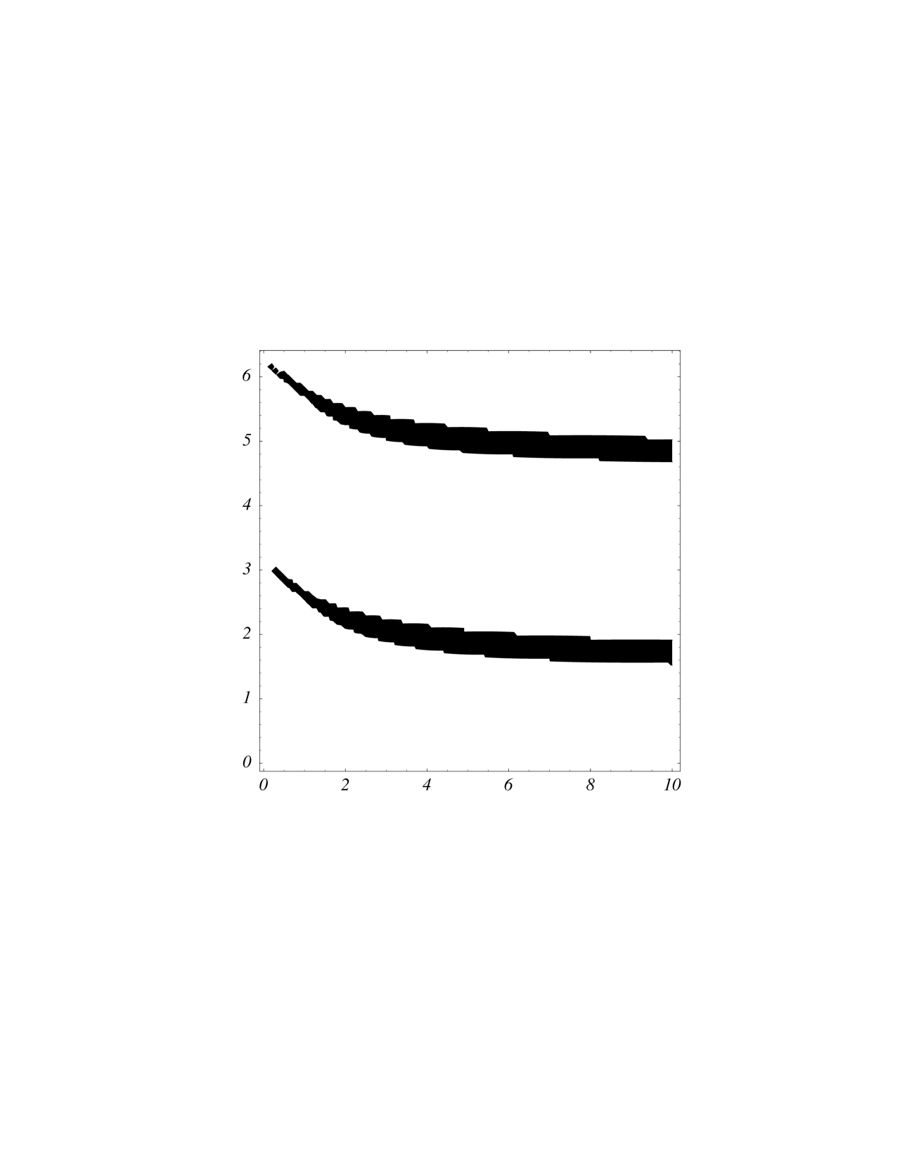
Figure 1: The $F(y,\theta)=0$ contour in the $(y,\theta)$ plane.

References

- [1] J.-M. Frère, D.R.T. Jones and S. Raby, Nucl. Phys. B222 (1983) 11; M. Claudson, L. Hall and I. Hinchcliffe, Nucl. Phys. B228 (1983) 501; H.-P. Nilles, M. Srednicki and D. Wyler, Phys. Lett. B120 (1983) 346; J-P. Derendinger and C. A. Savoy, Nucl. Phys. B237 (1984) 307; H. Komatsu, Phys. Lett. B215 (1988) 323; P. Langacker and N. Polonsky, Phys. Rev. D50 (1994) 2199; A. Kusenko, P. Langacker and G. Segre, Phys. Rev. D54 (1996) 5824; J.A. Casas and S. Dimopoulos, Phys. Lett. B387 (1996) 107; J.A. Casas, hep-ph/9707475 ; J.A. Casas, A. Lleyda and C. Munoz, Nucl. Phys. B471 (1996) 3; J.A. Casas, A. Lleyda and C. Munoz, Phys. Lett. B389 (1996) 305.
- [2] J.A. Casas, A. Lleyda and C. Munoz, Phys. Lett. B380 (1996) 59; S.A. Abel and B.C. Allanach, Phys. Lett. B415 (371) 1997; Phys. Lett. B431 (1998) 339; I. Dasgupta, R. Rademacher and P. Suranyi, hep-ph/9804229
- [3] T. Falk, K.A. Olive, L. Roszkowski and M. Srednicki, Phys. Lett. B367 (1996) 183; A. Riotto and E. Roulet, Phys. Lett. B377 (1996) 60; A. Strumia, Nucl. Phys. B482 (1996) 24; T. Falk, K.A. Olive, L. Roszkowski, A. Singh and M. Srednicki, Phys. Lett. B396 (1997) 50
- [4] S.A. Abel and C.A. Savoy, hep-ph/9803218
- [5] F. Buccella, J-P. Derendinger, C.A. Savoy and S. Ferrara, Phys. Lett. B115 (1982) 375; R. Gatto and G. Sartori, Phys. Lett. B157 (1985) 389; M.A. Luty and W. Taylor, Phys. Rev. D53 (1996) 3399
- [6] T. Ghergetta, C. Kolda, S.P. Martin, Nucl. Phys. B468 (1996) 37.
- [7] P. Horava and E. Witten, Nucl. Phys. B475 (1996) 94; E. Witten, Nucl. Phys. B471 (1996) 135; P. Horava, Phys. Rev. D54 (1996) 7561;
- [8] I. Antoniadis and M. Quiros, Phys. Lett. B392 (1997) 61; Nucl. Phys. B505 (1997) 109; Phys. Lett. B416 (1998) P327; E. Dudas and J.C. Grojean, Nucl. Phys. B507 (1997) 553; E. Dudas, Phys. Lett. B416 (1998) 309; Z. Lalak and S. Thomas, Nucl. Phys. B515 (1998) 55; T. Li, J.L. Lopez and D.V. Nanopoulos, Mod. Phys. Lett. A 12 (1997) 2647; H.P. Nilles, M. Olechowski and M. Yamguchi, Phys. Lett. B415 (1997) 24; hep-th/9801030; A. Lukas, B.A. Ovrut and D. Waldram, Phys. Rev. D57 (1998) 7529; D. Bailin, G.V. Kraniotis and A. Love, hep-ph/9803274; J. Ellis, Z. Lalak, S. Pokorski and W Pokorski hep-ph/9805377 ; I. Antoniadis, E. Dudas, A. Sagnotti, hep-th/9807011 ; E.A. Mirabelli and M.E. Peskin, Phys. Rev. D58 (1998) 65; T. Li, Phys. Rev. D57 (1998) 7539
- [9] K. Choi, H.B. Kim and C. Munoz, Phys. Rev. D57 (1998) 7521