DTP/98/58

September 1998


Four jet event shapes in electron-positron annihilation
J. M. Campbell, M. A. Cullen and E. W. N. Glover Department of Physics, University of Durham, Durham DH1 3LE, England

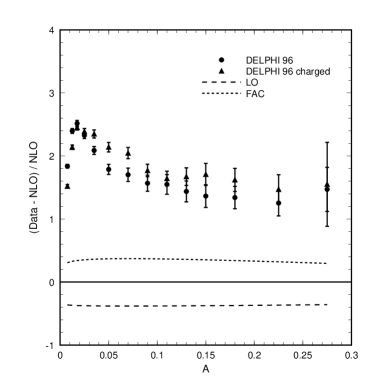
We report next-to-leading order perturbative QCD predictions of 4 jet event shape variables for the process e+e4jetssuperscript𝑒superscript𝑒4jetse^{+}e^{-}\to\rm{4\,\,jets} obtained using the general purpose Monte Carlo EERAD2. This program is based on the known ‘squared’ one loop matrix elements for the virtual γ4superscript𝛾4\gamma^{*}\to 4 parton contribution and squared matrix elements for 5 parton production. To combine the two distinct final states numerically we present a hybrid of the commonly used subtraction and slicing schemes based on the colour antenna structure of the final state which can be readily applied to other processes. We have checked that the numerical results obtained with EERAD2 are consistent with next-to-leading order estimates of the distributions of previously determined four jet-like event variables. We also report the next-to-leading order scale independent coefficients for some previously uncalculated observables; the light hemisphere mass, narrow jet broadening, Aplanarity and the 4 jet transition variables with respect to the JADE and Geneva jet finding algorithms. For each of these observables, the next-to-leading order corrections calculated at the physical scale significantly increase the rate compared to leading order (the K factor is approximately 1.5 – 2). With the exception of the 4 jet transition variables, the published DELPHI data lies well above the 𝒪(αs3)𝒪superscriptsubscript𝛼𝑠3{\cal O}(\alpha_{s}^{3}) predictions. The renormalisation scale uncertainty is still large and in most cases the data prefers a scale significantly smaller than the physical scale. This situation is reminiscent of that for three jet shape variables, and should be improved by the inclusion of power corrections and resummation of large infrared logarithms.

1 Introduction

Electron-positron colliders, in particular those at both LEP and SLAC, have provided much precision data with which to probe the structure of QCD. This is particularly valuable data because the strong interactions occur only in the final state and are not entangled with the parton density functions associated with beams of hadrons. In addition to measuring multi-jet production rates, more specific information about the topology of the events can be extracted. To this end, many variables have been introduced which characterize the hadronic structure of an event. For example, we can ask how planar or how collimated an event is. In general, a variable is described as n𝑛n jet-like if it vanishes for a final state configuration of n1𝑛1n-1 hadrons. With the precision data from LEP and SLC, experimental distributions for such event shape variables have been studied and have been compared where possible with theoretical calculations.

Generally speaking, leading order (LO) predictions successfully predict the general features of distributions, but can be improved by resumming kinematically-dominant logarithms, by including more perturbative information or both. A next-to-leading order (NLO) treatment of three-jet like variables was first performed in [1, 2] and systematically completed in [3]. Armed with such calculations, one can extract a value for the strong coupling αssubscript𝛼𝑠\alpha_{s} either directly from the event shape distributions [4] or from the energy dependence of their average value [5]. Alternatively, one can study the group parameters of the gauge theory of the strong interactions [6], though for three jet observables, the gluon-gluon coupling (proportional to CAsubscript𝐶𝐴C_{A}) occurs first at NLO.

Recent calculations of the relevant one-loop four parton matrix elements for γ4superscript𝛾4\gamma^{*}\to 4 partons [7] and e+e4superscript𝑒superscript𝑒4e^{+}e^{-}\to 4 partons [8], together with the known tree-level five parton matrix elements [9] have enabled the phenomenology of four-jet production to be be studied at next-to-leading order. So far, two groups have used these matrix elements to construct general purpose Monte Carlo programs for four jet-like quantities MENLO PARC [10] and DEBRECEN [11], which have been used to measure the four jet fraction R4subscript𝑅4R_{4} and a variety of event shape distributions [11]. We note that four jet production is sensitive to the casimir structure of QCD [12, 8] and four jet events may be used to constrain the allowed values of CFsubscript𝐶𝐹C_{F}, CAsubscript𝐶𝐴C_{A} and TRsubscript𝑇𝑅T_{R} [13] by examining the angles between the jets [14]. One may also place next-to-leading order bounds on the possible presence of the elusive light gluino present in many supersymmetric models [15].

Any such Monte Carlo program must suitably combine the virtual four parton and real five parton pieces of the cross section. That is,

σNLO=dσ4+dσ5=dPS4|4|2+dPS5|5|2,subscript𝜎NLOdifferential-dsubscript𝜎4differential-dsubscript𝜎5differential-d𝑃subscript𝑆4superscriptsubscript42differential-d𝑃subscript𝑆5superscriptsubscript52\sigma_{\rm NLO}=\int{\rm d}\sigma_{4}+\int{\rm d}\sigma_{5}=\int{\rm d}PS_{4}\,|{\cal M}_{4}|^{2}+\int{\rm d}PS_{5}\,|{\cal M}_{5}|^{2}, (1.1)

where the n𝑛n-parton contributions dσndsubscript𝜎𝑛{\rm d}\sigma_{n} are integrals over the n𝑛n-parton phase-space dPSnd𝑃subscript𝑆𝑛{\rm d}PS_{n}. Both integrals are separately divergent, and contain both infrared and ultraviolet singularities. The ultraviolet poles are removed by renormalisation, however the soft and collinear infrared poles are only cancelled when the virtual graphs are combined with the bremstrahlung process and one must provide a means to cancel the infrared singularities caused by two particles becoming collinear or one soft. Although the cancellation of infrared poles can be done analytically for simple processes, for complicated processes, it is necessary to resort to numerical techniques. A variety of methods - known as subtraction [1, 16, 17], slicing [2, 18] and hybrid subtraction [19] - are in general use, and variations of the subtraction formalism have been implemented in [10, 11]. Here we report on results obtained using a third numerical implementation of these matrix elements to compute generic infrared safe four jet observables. We call this program EERAD2 [20] and it is based on the ‘squared’ one-loop matrix elements for γ4superscript𝛾4\gamma^{*}\to 4 partons of [7] together with squared tree level matrix elements for γ5superscript𝛾5\gamma^{*}\to 5 partons. To isolate and cancel the infrared singularities, we use a hybrid approach that contains elements of both slicing and subtraction methods. In particular, we use an antenna factorisation where two (colour connected) hard partons radiate a third that may be unresolved. This is necessarily a rather technical subject and it is detailed in the appendix.

For the bulk of the paper we are more concerned with the phenomenology of four jet-like shape variables and, in particular, we extend the set of variables that have been computed at 𝒪(αs3)𝒪superscriptsubscript𝛼𝑠3{\cal O}(\alpha_{s}^{3}).111Some of the results presented here have been reported in [21]. To be precise, we present next-to-leading order coefficents for the differential distributions of the narrow jet broadening, light hemisphere mass, Aplanarity and the jet transition variable for the JADE and Geneva jet algorithms. To compare with previous results, we also consider the thrust minor, D𝐷D parameter and the jet transition variable for the Durham jet algorithm as well as the four jet rate as a function of the jet resolution parameter ycutsubscript𝑦cuty_{\rm cut}.

In section 2, we give the definitions of the relevant four jet shape variables and review the structure of the perturbative predictions. Section 3 shows the consistency of our program, by reproducing the known four-jet fraction and D𝐷D parameter distributions. The main results are reported in section 4 and comparisons with experimental data follow in section 5, where we also discuss how we might optimize our perturbative input by choice of a suitable renormalization scale. Conclusions are summarized in section 6. Finally, a more detailed discussion of our method for cancellation of the infrared singularities is reserved for the Appendix.

2 Four jet event shapes

The sorts of variables we are interested in are four jet-like, since they can only be non-zero for final states in which there are four or more particles. They usually rely on the hadronic final state having some volume and, when the event is coplanar, some observables like the D𝐷D parameter are identically zero.

2.1 Definition of Variables

In the following definitions, the sums run over all N𝑁N final state particles, k=1,,N𝑘1𝑁k=1,\ldots,N. pksubscript𝑝𝑘\vec{p}_{k} is the three-momentum of particle k𝑘k in the c.m. frame, with components pkisuperscriptsubscript𝑝𝑘𝑖p_{k}^{i}, i=1,2,3𝑖123i=1,2,3.

  • (a)

    C𝐶C and D𝐷D parameters [22].
    We first construct the linear momentum tensor,

    Θij=kpkipkj|pk|k|pk|,superscriptΘ𝑖𝑗subscript𝑘subscriptsuperscript𝑝𝑖𝑘subscriptsuperscript𝑝𝑗𝑘subscript𝑝𝑘subscript𝑘subscript𝑝𝑘\Theta^{ij}=\frac{\sum_{k}\frac{p^{i}_{k}p^{j}_{k}}{|\vec{p}_{k}|}}{\sum_{k}|\vec{p_{k}}|}, (2.1)

    with eigenvalues λisubscript𝜆𝑖\lambda_{i} for i=1,2,3𝑖123i=1,2,3. The normalisation is such that iλi=1subscript𝑖subscript𝜆𝑖1\sum_{i}\lambda_{i}=1. For planar events one of the eigenvalues is zero. The C𝐶C and D𝐷D parameters are defined by,

    D=27λ1λ2λ3,𝐷27subscript𝜆1subscript𝜆2subscript𝜆3D=27\lambda_{1}\lambda_{2}\lambda_{3}, (2.2)

    and,

    C=3(λ1λ2+λ2λ3+λ3λ1).𝐶3subscript𝜆1subscript𝜆2subscript𝜆2subscript𝜆3subscript𝜆3subscript𝜆1C=3(\lambda_{1}\lambda_{2}+\lambda_{2}\lambda_{3}+\lambda_{3}\lambda_{1}). (2.3)

    D𝐷D can only be non-zero for non-planar four (or more) parton events, while three parton events may produce 0C0.750𝐶0.750\leq C\leq 0.75. Only the region C>0.75𝐶0.75C>0.75 should be considered four jet-like.

  • (b)

    Thrust minor, Tminorsubscript𝑇minorT_{{\rm minor}} [23].
    We first define the thrust, major and minor axes (n1,n2,n3subscript𝑛1subscript𝑛2subscript𝑛3\vec{n}_{1},\vec{n}_{2},\vec{n}_{3}) by,

    Ti=maxnik|pknk|k|pk|,subscript𝑇𝑖subscriptsubscript𝑛𝑖subscript𝑘subscript𝑝𝑘subscript𝑛𝑘subscript𝑘subscript𝑝𝑘T_{i}=\max_{\vec{n}_{i}}\frac{\sum_{k}|\vec{p}_{k}\cdot\vec{n}_{k}|}{\sum_{k}|\vec{p}_{k}|}, (2.4)

    where n2subscript𝑛2\vec{n}_{2} is constrained by n1n2=0subscript𝑛1subscript𝑛20\vec{n}_{1}\cdot\vec{n}_{2}=0. and n3=n1×n2subscript𝑛3subscript𝑛1subscript𝑛2\vec{n}_{3}=\vec{n}_{1}\times\vec{n}_{2}.

  • (c)

    Light hemisphere mass, ML2/ssuperscriptsubscript𝑀𝐿2𝑠M_{L}^{2}/s.
    The event is separated into two hemispheres H1subscript𝐻1H_{1}, H2subscript𝐻2H_{2} divided by the plane normal to the thrust axis n1subscript𝑛1\vec{n}_{1}, as defined above. Particles that satisfy pi.n1>0formulae-sequencesubscript𝑝𝑖subscript𝑛10\vec{p}_{i}.\vec{n}_{1}>0 are assigned to hemisphere H1subscript𝐻1H_{1}, while all other particles are in H2subscript𝐻2H_{2}. Then,

    ML2s=1smini=1,2(pkHipk)2.\frac{M_{L}^{2}}{s}=\frac{1}{s}\cdot\min_{i=1,2}\left(\sum_{\vec{p}_{k}\in H_{i}}p_{k}\right)^{2}. (2.5)

    Note that this is the common modification of the original definition suggested by Clavelli [24].

  • (d)

    Narrow jet broadening, Bminsubscript𝐵minB_{{\rm min}} [25].
    Using the same division into hemispheres as above, we define,

    Bmin=mini=1,2pkHi|pk×n|2k|pk|.subscript𝐵minsubscript𝑖12subscriptsubscript𝑝𝑘subscript𝐻𝑖subscript𝑝𝑘𝑛2subscript𝑘subscript𝑝𝑘B_{\rm min}=\min_{i=1,2}\frac{\sum_{\vec{p}_{k}\in H_{i}}|\vec{p}_{k}\times\vec{n}|}{2\sum_{k}|\vec{p}_{k}|}. (2.6)
  • (e)

    Aplanarity, A𝐴A [26].
    Here we consider the eigenvalues, λ1λ2λ3subscript𝜆1subscript𝜆2subscript𝜆3\lambda_{1}\geq\lambda_{2}\geq\lambda_{3} of the quadratic momentum tensor,

    Φij=kpkipkjk|pk|2.superscriptΦ𝑖𝑗subscript𝑘subscriptsuperscript𝑝𝑖𝑘subscriptsuperscript𝑝𝑗𝑘subscript𝑘superscriptsubscript𝑝𝑘2\Phi^{ij}=\frac{\sum_{k}p^{i}_{k}p^{j}_{k}}{\sum_{k}|\vec{p}_{k}|^{2}}. (2.7)

    Aplanarity is defined by,

    A=32λ3,𝐴32subscript𝜆3A=\frac{3}{2}\lambda_{3}, (2.8)

    which is clearly zero for planar three particle events.

  • (f)

    Jet transition variable y4Ssuperscriptsubscript𝑦4𝑆y_{4}^{S}.
    The y4Ssuperscriptsubscript𝑦4𝑆y_{4}^{S} variable denotes the value of the jet resolution parameter ycutsubscript𝑦cuty_{\rm cut} at which an event changes from a four jet event to a three jet event where the jets are defined according to algorithm S𝑆S. We consider three algorithms, the JADE algorithm (S=J𝑆𝐽S=J) [27], the Durham algorithm (S=D𝑆𝐷S=D) [28] and the Geneva algorithm (S=G𝑆𝐺S=G) [29]. The jet-finding measures for each of these three algorithms are as follows,

    yijJ=2EiEj(1cosθij)s,subscriptsuperscript𝑦𝐽𝑖𝑗2subscript𝐸𝑖subscript𝐸𝑗1subscript𝜃𝑖𝑗𝑠\displaystyle y^{J}_{ij}=\frac{2\,E_{i}E_{j}(1-\cos\theta_{ij})}{s},
    yijD=2min(Ei2,Ej2)(1cosθij)s,subscriptsuperscript𝑦𝐷𝑖𝑗2superscriptsubscript𝐸𝑖2superscriptsubscript𝐸𝑗21subscript𝜃𝑖𝑗𝑠\displaystyle y^{D}_{ij}=\frac{2\,\min(E_{i}^{2},E_{j}^{2})(1-\cos\theta_{ij})}{s},
    yijG=89EiEj(1cosθij)(Ei+Ej)2,subscriptsuperscript𝑦𝐺𝑖𝑗89subscript𝐸𝑖subscript𝐸𝑗1subscript𝜃𝑖𝑗superscriptsubscript𝐸𝑖subscript𝐸𝑗2\displaystyle y^{G}_{ij}=\frac{8}{9}\frac{E_{i}E_{j}(1-\cos\theta_{ij})}{(E_{i}+E_{j})^{2}}, (2.9)

    where the factor of 8/9898/9 in the Geneva algorithm is simply to ensure that the maximum value of ycutsubscript𝑦cuty_{\rm{cut}} that reconstructs three jets from three partons is 1/3131/3 as it is for the other two algorithms. When particles combine, there is some ambiguity as to how to add the energies and momenta. In all three schemes, we use the E scheme i.e. we merely add four momenta,

    pijμ=piμ+pjμ.superscriptsubscript𝑝𝑖𝑗𝜇superscriptsubscript𝑝𝑖𝜇superscriptsubscript𝑝𝑗𝜇p_{ij}^{\mu}=p_{i}^{\mu}+p_{j}^{\mu}. (2.10)

    Other choices such as the E0 or P schemes where the cluster is made massless by rescaling the momentum or energy give similar results.

Of these variables, the D𝐷D, C𝐶C, Tminorsubscript𝑇minorT_{\rm minor} and y4Dsuperscriptsubscript𝑦4𝐷y_{4}^{D} distributions have been studied in [11].

2.2 Structure of Perturbative Prediction

The differential cross-section at centre-of-mass energy s𝑠\sqrt{s} for one of these four-jet variables (O4subscript𝑂4O_{4}) at next-to-leading order is described by two coefficients, BO4subscript𝐵subscript𝑂4B_{O_{4}} and CO4subscript𝐶subscript𝑂4C_{O_{4}} which represent the leading and next-to-leading order perturbative contributions,

1σ0O4dσdO4=(αs(μ)2π)2BO4+(αs(μ)2π)3(2β0log(μ2s)BO4+CO4).1subscript𝜎0subscript𝑂4𝑑𝜎𝑑subscript𝑂4superscriptsubscript𝛼𝑠𝜇2𝜋2subscript𝐵subscript𝑂4superscriptsubscript𝛼𝑠𝜇2𝜋32subscript𝛽0superscript𝜇2𝑠subscript𝐵subscript𝑂4subscript𝐶subscript𝑂4\frac{1}{\sigma_{0}}\cdot O_{4}\,\frac{d\sigma}{dO_{4}}=\left(\frac{\alpha_{s}(\mu)}{2\pi}\right)^{2}B_{O_{4}}+\left(\frac{\alpha_{s}(\mu)}{2\pi}\right)^{3}\left(2\beta_{0}\log\left(\frac{\mu^{2}}{s}\right)B_{O_{4}}+C_{O_{4}}\right). (2.11)

Both BO4subscript𝐵subscript𝑂4B_{O_{4}} and CO4subscript𝐶subscript𝑂4C_{O_{4}} are scale independent and do not depend on the beam energy. However, the running coupling αssubscript𝛼𝑠\alpha_{s} is calculated at renormalization scale μ𝜇\mu which is commonly chosen to be the physical scale, μ=s𝜇𝑠\mu=\sqrt{s}. Compared to the leading order prediction, which decays monotonically with increasing μ𝜇\mu, the next-to-leading order term reduces the scale dependence somewhat through the first coefficient of the beta-function, β0=(332Nf)/ 6subscript𝛽0332subscript𝑁𝑓6\beta_{0}=(33-2N_{f})/\,6. For five active quark flavours, β0=3.833subscript𝛽03.833\beta_{0}=3.833.

The individual coefficients BO4subscript𝐵subscript𝑂4B_{O_{4}} and CO4subscript𝐶subscript𝑂4C_{O_{4}} depend on the number of colours and flavours, or equivalently, the group casimirs of the standard model. As such, four jet event shapes may be used to simultaneously constrain the strong interaction gauge group as well as the strong coupling constant.

2.3 Scale choice and theoretical uncertainty

As mentioned above, for hadronic observables in electron-positron annihilation it is common to choose the renormalisation scale to be the physical scale μ=s𝜇𝑠\mu=\sqrt{s}. This choice is motivated by naturalness arguments and the fact that choosing a scale far from s𝑠\sqrt{s} introduces large logarithms of the form log(μ/s)𝜇𝑠\log(\mu/\sqrt{s}) in eq. (2.11). Since the renormalisation scale is only a theoretical construct, it has become common practice to estimate the uncertainty engendered by truncating the perturbative expansion by varying μ𝜇\mu by factors about the physical scale.

Other approaches have been considered with rather different scale choices. One such approach is to stipulate that the next-to-leading order coefficient vanishes. That is to say that the LO and NLO predictions coincide.222In other words, the ratio of NLO to LO predictions commonly called the K-factor is identically unity. This occurs at the scale,

μFAC=sexp(CO44BO4β0),superscript𝜇𝐹𝐴𝐶𝑠subscript𝐶subscript𝑂44subscript𝐵subscript𝑂4subscript𝛽0\mu^{FAC}=\sqrt{s}~{}\exp\left(-\frac{C_{O_{4}}}{4B_{O_{4}}\beta_{0}}\right), (2.12)

and is called the scale of fastest apparent convergence (FAC) [30]. As we will see, CO4subscript𝐶subscript𝑂4C_{O_{4}} is typically 50-100 times larger than BO4subscript𝐵subscript𝑂4B_{O_{4}} so that μFACsuperscript𝜇𝐹𝐴𝐶\mu^{FAC} may be as small as 102superscript10210^{-2}103superscript10310^{-3} of the physical scale.

Another common choice is to select the scale where the NLO prediction is most insensitive to the choice of scale [31]. However, this scale is very close to the FAC scale (15% smaller) so that the Principle of Minimal Sensitivity scale (PMS) predictions lie very close to the FAC scale prediction.

While even higher order corrections remain uncalculated, varying the renormalisation scale can only give a crude indication of the theoretical uncertainty. Therefore, in an attempt to make a fair estimate of the theoretical uncertainty on the NLO prediction we will show both the physical scale and FAC scale predictions.

2.4 Infrared behaviour

Four jet event shapes typically depend on the event having some volume and not lying entirely in a plane. Typical hadronic events contain more than 20 hadrons and it is extremely unlikely that the value of any event shape is precisely zero for any experimental event.However, in a LO or NLO fixed order parton calculation, there only four or five partons present in the final state and, when one or more are soft, the calculated O4subscript𝑂4O_{4} may approach zero. In such circumstances, soft gluon singularities cause the fixed order prediction to become wildly unstable and grow logarithmically. In the small O4subscript𝑂4O_{4} limits, the perturbative coefficients have the following form,

BO4subscript𝐵subscript𝑂4\displaystyle B_{O_{4}} \displaystyle\to A32L3+A22L2+A12L+A02,subscript𝐴32superscript𝐿3subscript𝐴22superscript𝐿2subscript𝐴12𝐿subscript𝐴02\displaystyle A_{32}L^{3}+A_{22}L^{2}+A_{12}L+A_{02},
CO4subscript𝐶subscript𝑂4\displaystyle C_{O_{4}} \displaystyle\to A53L5+A43L4+A33L3+A23L2+A13L+A03,subscript𝐴53superscript𝐿5subscript𝐴43superscript𝐿4subscript𝐴33superscript𝐿3subscript𝐴23superscript𝐿2subscript𝐴13𝐿subscript𝐴03\displaystyle A_{53}L^{5}+A_{43}L^{4}+A_{33}L^{3}+A_{23}L^{2}+A_{13}L+A_{03}, (2.13)

where L=log(1/O4)𝐿1subscript𝑂4L=\log(1/O_{4}) and Anmsubscript𝐴𝑛𝑚A_{nm} are (as yet) undetermined coefficients. Whenever L𝐿L is sufficiently large, resummation effects will be important.333Whether the coefficients exponentiate and can be resummed will depend on the observable. In comparing with data, we therefore choose to make a cut on the size of O4subscript𝑂4O_{4} which is typically in the range 0.001 — 0.01, since for such small values of O4subscript𝑂4O_{4} we do not trust the NLO prediction. In comparing with the DELPHI data, this cut will usually be the lower edge of the second data bin.

3 Comparison with existing results

3.1 Four jet rates

As a check of the numerical results, Table 1 shows the predictions for each of the three Monte Carlo programs for the four jet rate for three jet clustering algorithms; the Jade-E0, Durham-E [28], and Geneva-E [29] algorithms. We show results with αs(MZ)=0.118subscript𝛼𝑠subscript𝑀𝑍0.118\alpha_{s}(M_{Z})=0.118 for three values of the jet resolution parameter ycutsubscript𝑦𝑐𝑢𝑡y_{cut}. There is good agreement with the results from the other two calculations.

Algorithm ycutsubscript𝑦cuty_{{\rm cut}} MENLO PARC DEBRECEN EERAD2
0.005 (1.04±0.02)101plus-or-minus1.040.02superscript101(1.04\pm 0.02)\cdot 10^{-1} (1.05±0.01)101plus-or-minus1.050.01superscript101(1.05\pm 0.01)\cdot 10^{-1} (1.05±0.01)101plus-or-minus1.050.01superscript101(1.05\pm 0.01)\cdot 10^{-1}
Durham 0.01 (4.70±0.06)102plus-or-minus4.700.06superscript102(4.70\pm 0.06)\cdot 10^{-2} (4.66±0.02)102plus-or-minus4.660.02superscript102(4.66\pm 0.02)\cdot 10^{-2} (4.65±0.02)102plus-or-minus4.650.02superscript102(4.65\pm 0.02)\cdot 10^{-2}
0.03 (6.82±0.08)103plus-or-minus6.820.08superscript103(6.82\pm 0.08)\cdot 10^{-3} (6.87±0.04)103plus-or-minus6.870.04superscript103(6.87\pm 0.04)\cdot 10^{-3} (6.86±0.03)103plus-or-minus6.860.03superscript103(6.86\pm 0.03)\cdot 10^{-3}
0.02 (2.56±0.06)101plus-or-minus2.560.06superscript101(2.56\pm 0.06)\cdot 10^{-1} (2.63±0.06)101plus-or-minus2.630.06superscript101(2.63\pm 0.06)\cdot 10^{-1} (2.61±0.05)101plus-or-minus2.610.05superscript101(2.61\pm 0.05)\cdot 10^{-1}
Geneva 0.03 (1.71±0.03)101plus-or-minus1.710.03superscript101(1.71\pm 0.03)\cdot 10^{-1} (1.75±0.03)101plus-or-minus1.750.03superscript101(1.75\pm 0.03)\cdot 10^{-1} (1.72±0.03)101plus-or-minus1.720.03superscript101(1.72\pm 0.03)\cdot 10^{-1}
0.05 (8.58±0.15)102plus-or-minus8.580.15superscript102(8.58\pm 0.15)\cdot 10^{-2} (8.37±0.12)102plus-or-minus8.370.12superscript102(8.37\pm 0.12)\cdot 10^{-2} (8.50±0.06)102plus-or-minus8.500.06superscript102(8.50\pm 0.06)\cdot 10^{-2}
0.005 (3.79±0.08)101plus-or-minus3.790.08superscript101(3.79\pm 0.08)\cdot 10^{-1} (3.88±0.07)101plus-or-minus3.880.07superscript101(3.88\pm 0.07)\cdot 10^{-1} (3.87±0.03)101plus-or-minus3.870.03superscript101(3.87\pm 0.03)\cdot 10^{-1}
JADE-E0 0.01 (1.88±0.03)101plus-or-minus1.880.03superscript101(1.88\pm 0.03)\cdot 10^{-1} (1.92±0.01)101plus-or-minus1.920.01superscript101(1.92\pm 0.01)\cdot 10^{-1} (1.93±0.01)101plus-or-minus1.930.01superscript101(1.93\pm 0.01)\cdot 10^{-1}
0.03 (3.46±0.05)102plus-or-minus3.460.05superscript102(3.46\pm 0.05)\cdot 10^{-2} (3.37±0.01)102plus-or-minus3.370.01superscript102(3.37\pm 0.01)\cdot 10^{-2} (3.35±0.01)102plus-or-minus3.350.01superscript102(3.35\pm 0.01)\cdot 10^{-2}
Table 1: The four-jet fraction as calculated by MENLO PARC, DEBRECEN and EERAD2, for the different jet recombination schemes and varying ycutsubscript𝑦cuty_{\rm cut}. The rate is normalized by the 𝒪(αs)𝒪subscript𝛼𝑠{\cal O}(\alpha_{s}) total hadronic cross-section, σhad=σ0(1+αs/π)subscript𝜎hadsubscript𝜎01subscript𝛼𝑠𝜋\sigma_{\rm had}=\sigma_{0}\,(1+\alpha_{s}/\pi).

3.2 Shape variables

As mentioned earlier, Nagy and Trócsányi [11] have computed CDsubscript𝐶𝐷C_{D} with their Monte Carlo DEBRECEN. In Table 2 we show the leading and next-to-leading order coefficients BDsubscript𝐵𝐷B_{D} and CDsubscript𝐶𝐷C_{D} calculated by EERAD2, together with the DEBRECEN result. The two calculations are clearly consistent with one another, with the quoted errors overlapping in almost all cases. The errors from EERAD2 are of the order of 2% in each bin, except in the tail of the distribution where the errors rise as high as 10%. The infrared enhancement of the distribution described in section 2.4 means that the Monte Carlo procedure favours the phase space region corresponding to small values of the D𝐷D parameter, so that the large D𝐷D tail suffers larger errors. In fact CDsubscript𝐶𝐷C_{D} drops by four orders of magnitude over the kinematic range of the observable so it is necessary to use importance sampling with respect to the observable distribution to ensure sufficient Monte Carlo points are produced in the high D𝐷D region. This is also true for all of the other shape variables.

In addition, Nagy and Trócsányi have also presented results for the next-to-leading order coefficents for thrust minor Tminorsubscript𝑇minorT_{\rm minor} and the jet transition variable in the Durham scheme y4Dsuperscriptsubscript𝑦4𝐷y_{4}^{D} [11]. Although we do not present a detailed comparison here, we note that the agreement is qualitatively the same as discussed for the D𝐷D parameter above. We find that the distributions extend beyond the range of coefficents presented in [11], with non-zero coefficients for bins in the ranges 0.5<Tminor<0.580.5subscript𝑇minor0.580.5<T_{\rm minor}<0.58 and 0.125<y4D<0.170.125superscriptsubscript𝑦4𝐷0.170.125<y_{4}^{D}<0.17.

D𝐷D BDsubscript𝐵𝐷B_{D} CDsubscript𝐶𝐷C_{D} DEBRECEN
0.0200 (3.79±0.01)102plus-or-minus3.790.01superscript102(3.79\pm 0.01)\cdot 10^{2} (1.47±0.00)104plus-or-minus1.470.00superscript104(1.47\pm 0.00)\cdot 10^{4} (1.08±0.06)104plus-or-minus1.080.06superscript104(1.08\pm 0.06)\cdot 10^{4}
0.0600 (2.32±0.01)102plus-or-minus2.320.01superscript102(2.32\pm 0.01)\cdot 10^{2} (1.25±0.01)104plus-or-minus1.250.01superscript104(1.25\pm 0.01)\cdot 10^{4} (1.24±0.02)104plus-or-minus1.240.02superscript104(1.24\pm 0.02)\cdot 10^{4}
0.1000 (1.45±0.01)102plus-or-minus1.450.01superscript102(1.45\pm 0.01)\cdot 10^{2} (8.69±0.04)103plus-or-minus8.690.04superscript103(8.69\pm 0.04)\cdot 10^{3} (8.59±0.12)103plus-or-minus8.590.12superscript103(8.59\pm 0.12)\cdot 10^{3}
0.1400 (1.04±0.01)102plus-or-minus1.040.01superscript102(1.04\pm 0.01)\cdot 10^{2} (6.39±0.03)103plus-or-minus6.390.03superscript103(6.39\pm 0.03)\cdot 10^{3} (6.24±0.12)103plus-or-minus6.240.12superscript103(6.24\pm 0.12)\cdot 10^{3}
0.1800 (7.68±0.04)101plus-or-minus7.680.04superscript101(7.68\pm 0.04)\cdot 10^{1} (4.89±0.03)103plus-or-minus4.890.03superscript103(4.89\pm 0.03)\cdot 10^{3} (4.99±0.11)103plus-or-minus4.990.11superscript103(4.99\pm 0.11)\cdot 10^{3}
0.2200 (5.87±0.03)101plus-or-minus5.870.03superscript101(5.87\pm 0.03)\cdot 10^{1} (3.88±0.03)103plus-or-minus3.880.03superscript103(3.88\pm 0.03)\cdot 10^{3} (3.85±0.06)103plus-or-minus3.850.06superscript103(3.85\pm 0.06)\cdot 10^{3}
0.2600 (4.66±0.07)101plus-or-minus4.660.07superscript101(4.66\pm 0.07)\cdot 10^{1} (3.04±0.03)103plus-or-minus3.040.03superscript103(3.04\pm 0.03)\cdot 10^{3} (2.98±0.05)103plus-or-minus2.980.05superscript103(2.98\pm 0.05)\cdot 10^{3}
0.3000 (3.75±0.07)101plus-or-minus3.750.07superscript101(3.75\pm 0.07)\cdot 10^{1} (2.51±0.04)103plus-or-minus2.510.04superscript103(2.51\pm 0.04)\cdot 10^{3} (2.52±0.05)103plus-or-minus2.520.05superscript103(2.52\pm 0.05)\cdot 10^{3}
0.3400 (3.07±0.05)101plus-or-minus3.070.05superscript101(3.07\pm 0.05)\cdot 10^{1} (2.02±0.03)103plus-or-minus2.020.03superscript103(2.02\pm 0.03)\cdot 10^{3} (1.94±0.05)103plus-or-minus1.940.05superscript103(1.94\pm 0.05)\cdot 10^{3}
0.3800 (2.41±0.03)101plus-or-minus2.410.03superscript101(2.41\pm 0.03)\cdot 10^{1} (1.61±0.03)103plus-or-minus1.610.03superscript103(1.61\pm 0.03)\cdot 10^{3} (1.59±0.04)103plus-or-minus1.590.04superscript103(1.59\pm 0.04)\cdot 10^{3}
0.4200 (1.97±0.04)101plus-or-minus1.970.04superscript101(1.97\pm 0.04)\cdot 10^{1} (1.37±0.02)103plus-or-minus1.370.02superscript103(1.37\pm 0.02)\cdot 10^{3} (1.37±0.03)103plus-or-minus1.370.03superscript103(1.37\pm 0.03)\cdot 10^{3}
0.4600 (1.56±0.03)101plus-or-minus1.560.03superscript101(1.56\pm 0.03)\cdot 10^{1} (1.09±0.01)103plus-or-minus1.090.01superscript103(1.09\pm 0.01)\cdot 10^{3} (1.06±0.03)103plus-or-minus1.060.03superscript103(1.06\pm 0.03)\cdot 10^{3}
0.5000 (1.32±0.01)101plus-or-minus1.320.01superscript101(1.32\pm 0.01)\cdot 10^{1} (8.97±0.14)102plus-or-minus8.970.14superscript102(8.97\pm 0.14)\cdot 10^{2} (8.72±0.19)102plus-or-minus8.720.19superscript102(8.72\pm 0.19)\cdot 10^{2}
0.5400 (1.05±0.02)101plus-or-minus1.050.02superscript101(1.05\pm 0.02)\cdot 10^{1} (7.12±0.15)102plus-or-minus7.120.15superscript102(7.12\pm 0.15)\cdot 10^{2} (7.11±0.16)102plus-or-minus7.110.16superscript102(7.11\pm 0.16)\cdot 10^{2}
0.5800 (8.46±0.16)100plus-or-minus8.460.16superscript100(8.46\pm 0.16)\cdot 10^{0} (5.79±0.12)102plus-or-minus5.790.12superscript102(5.79\pm 0.12)\cdot 10^{2} (5.68±0.14)102plus-or-minus5.680.14superscript102(5.68\pm 0.14)\cdot 10^{2}
0.6200 (6.60±0.16)100plus-or-minus6.600.16superscript100(6.60\pm 0.16)\cdot 10^{0} (4.55±0.09)102plus-or-minus4.550.09superscript102(4.55\pm 0.09)\cdot 10^{2} (4.46±0.21)102plus-or-minus4.460.21superscript102(4.46\pm 0.21)\cdot 10^{2}
0.6600 (5.32±0.13)100plus-or-minus5.320.13superscript100(5.32\pm 0.13)\cdot 10^{0} (3.58±0.07)102plus-or-minus3.580.07superscript102(3.58\pm 0.07)\cdot 10^{2} (3.52±0.11)102plus-or-minus3.520.11superscript102(3.52\pm 0.11)\cdot 10^{2}
0.7000 (3.99±0.09)100plus-or-minus3.990.09superscript100(3.99\pm 0.09)\cdot 10^{0} (2.80±0.09)102plus-or-minus2.800.09superscript102(2.80\pm 0.09)\cdot 10^{2} (2.74±0.09)102plus-or-minus2.740.09superscript102(2.74\pm 0.09)\cdot 10^{2}
0.7400 (3.06±0.05)100plus-or-minus3.060.05superscript100(3.06\pm 0.05)\cdot 10^{0} (2.05±0.08)102plus-or-minus2.050.08superscript102(2.05\pm 0.08)\cdot 10^{2} (2.08±0.08)102plus-or-minus2.080.08superscript102(2.08\pm 0.08)\cdot 10^{2}
0.7800 (2.26±0.04)100plus-or-minus2.260.04superscript100(2.26\pm 0.04)\cdot 10^{0} (1.58±0.04)102plus-or-minus1.580.04superscript102(1.58\pm 0.04)\cdot 10^{2} (1.54±0.06)102plus-or-minus1.540.06superscript102(1.54\pm 0.06)\cdot 10^{2}
0.8200 (1.54±0.04)100plus-or-minus1.540.04superscript100(1.54\pm 0.04)\cdot 10^{0} (1.05±0.03)102plus-or-minus1.050.03superscript102(1.05\pm 0.03)\cdot 10^{2} (1.03±0.04)102plus-or-minus1.030.04superscript102(1.03\pm 0.04)\cdot 10^{2}
0.8600 (9.72±0.21)101plus-or-minus9.720.21superscript101(9.72\pm 0.21)\cdot 10^{-1} (6.72±0.29)101plus-or-minus6.720.29superscript101(6.72\pm 0.29)\cdot 10^{1} (6.66±0.31)101plus-or-minus6.660.31superscript101(6.66\pm 0.31)\cdot 10^{1}
0.9000 (5.63±0.16)101plus-or-minus5.630.16superscript101(5.63\pm 0.16)\cdot 10^{-1} (3.85±0.17)101plus-or-minus3.850.17superscript101(3.85\pm 0.17)\cdot 10^{1} (3.89±0.20)101plus-or-minus3.890.20superscript101(3.89\pm 0.20)\cdot 10^{1}
0.9400 (2.62±0.07)101plus-or-minus2.620.07superscript101(2.62\pm 0.07)\cdot 10^{-1} (1.71±0.10)101plus-or-minus1.710.10superscript101(1.71\pm 0.10)\cdot 10^{1} (1.71±0.19)101plus-or-minus1.710.19superscript101(1.71\pm 0.19)\cdot 10^{1}
0.9800 (5.34±0.11)102plus-or-minus5.340.11superscript102(5.34\pm 0.11)\cdot 10^{-2} (3.15±0.27)100plus-or-minus3.150.27superscript100(3.15\pm 0.27)\cdot 10^{0} (2.60±1.30)100plus-or-minus2.601.30superscript100(2.60\pm 1.30)\cdot 10^{0}
Table 2: The leading and next-to-leading order coefficients for the D𝐷D parameter. The NLO coefficient predicted by Nagy and Trócsányi Monte Carlo DEBRECEN [11] is also shown.

4 New results

In this section we extend the analysis of 4 jet-like event shape observables already found in the literature by reporting the leading and next-to-leading order coefficients for the light hemisphere mass, the narrow hemisphere broadening, Aplanarity and the jet transition variable in both the JADE and Geneva schemes, y4Jsuperscriptsubscript𝑦4𝐽y_{4}^{J} and y4Gsuperscriptsubscript𝑦4𝐺y_{4}^{G}. In particular, we examine the relative sizes of the two terms by inspecting the K factor (at the physical scale) for each variable across the allowed kinematic range of the distributions.

For all the variables presented in this section, we must be careful to differentiate between the true behaviour of the distribution as the observable tends to zero and the behaviour in fixed order perturbation theory. Each of the observables should have a smooth behaviour as O40subscript𝑂40O_{4}\to 0 rather than the divergent behaviour exhibited by the coefficients according to equation 2.13. To recover a smooth result in this limit it is necessary to resum powers of log(1/O4\log(1/O_{4}) where possible, a procedure which has been performed already for many 3 jet-like variables [32, 25]

4.1 Light Hemisphere Mass

ML2/ssuperscriptsubscript𝑀𝐿2𝑠M_{L}^{2}/s BML2/ssubscript𝐵superscriptsubscript𝑀𝐿2𝑠B_{M_{L}^{2}/s} CML2/ssubscript𝐶superscriptsubscript𝑀𝐿2𝑠C_{M_{L}^{2}/s}
0.0150 (3.23±0.08)102plus-or-minus3.230.08superscript102(3.23\pm 0.08)\cdot 10^{2} (1.41±0.01)104plus-or-minus1.410.01superscript104(1.41\pm 0.01)\cdot 10^{4}
0.0250 (1.88±0.02)102plus-or-minus1.880.02superscript102(1.88\pm 0.02)\cdot 10^{2} (8.85±0.10)103plus-or-minus8.850.10superscript103(8.85\pm 0.10)\cdot 10^{3}
0.0350 (1.25±0.02)102plus-or-minus1.250.02superscript102(1.25\pm 0.02)\cdot 10^{2} (5.97±0.11)103plus-or-minus5.970.11superscript103(5.97\pm 0.11)\cdot 10^{3}
0.0450 (8.52±0.10)101plus-or-minus8.520.10superscript101(8.52\pm 0.10)\cdot 10^{1} (4.14±0.08)103plus-or-minus4.140.08superscript103(4.14\pm 0.08)\cdot 10^{3}
0.0550 (5.97±0.06)101plus-or-minus5.970.06superscript101(5.97\pm 0.06)\cdot 10^{1} (3.04±0.04)103plus-or-minus3.040.04superscript103(3.04\pm 0.04)\cdot 10^{3}
0.0650 (4.20±0.09)101plus-or-minus4.200.09superscript101(4.20\pm 0.09)\cdot 10^{1} (2.15±0.05)103plus-or-minus2.150.05superscript103(2.15\pm 0.05)\cdot 10^{3}
0.0750 (3.02±0.07)101plus-or-minus3.020.07superscript101(3.02\pm 0.07)\cdot 10^{1} (1.58±0.05)103plus-or-minus1.580.05superscript103(1.58\pm 0.05)\cdot 10^{3}
0.0850 (2.13±0.03)101plus-or-minus2.130.03superscript101(2.13\pm 0.03)\cdot 10^{1} (1.11±0.02)103plus-or-minus1.110.02superscript103(1.11\pm 0.02)\cdot 10^{3}
0.0950 (1.39±0.04)101plus-or-minus1.390.04superscript101(1.39\pm 0.04)\cdot 10^{1} (7.66±0.23)102plus-or-minus7.660.23superscript102(7.66\pm 0.23)\cdot 10^{2}
0.1050 (8.75±0.20)100plus-or-minus8.750.20superscript100(8.75\pm 0.20)\cdot 10^{0} (4.97±0.17)102plus-or-minus4.970.17superscript102(4.97\pm 0.17)\cdot 10^{2}
0.1150 (5.18±0.13)100plus-or-minus5.180.13superscript100(5.18\pm 0.13)\cdot 10^{0} (3.27±0.07)102plus-or-minus3.270.07superscript102(3.27\pm 0.07)\cdot 10^{2}
0.1250 (2.59±0.12)100plus-or-minus2.590.12superscript100(2.59\pm 0.12)\cdot 10^{0} (1.66±0.07)102plus-or-minus1.660.07superscript102(1.66\pm 0.07)\cdot 10^{2}
0.1350 (8.97±0.35)101plus-or-minus8.970.35superscript101(8.97\pm 0.35)\cdot 10^{-1} (6.61±0.41)101plus-or-minus6.610.41superscript101(6.61\pm 0.41)\cdot 10^{1}
0.1450 (2.49±0.13)101plus-or-minus2.490.13superscript101(2.49\pm 0.13)\cdot 10^{-1} (1.79±0.09)101plus-or-minus1.790.09superscript101(1.79\pm 0.09)\cdot 10^{1}
0.1550 (5.00±0.27)102plus-or-minus5.000.27superscript102(5.00\pm 0.27)\cdot 10^{-2} (3.75±0.26)100plus-or-minus3.750.26superscript100(3.75\pm 0.26)\cdot 10^{0}
0.1650 (1.46±0.21)103plus-or-minus1.460.21superscript103(1.46\pm 0.21)\cdot 10^{-3} (2.30±0.37)101plus-or-minus2.300.37superscript101(2.30\pm 0.37)\cdot 10^{-1}
Table 3: The leading and next-to-leading order coefficients for the light jet mass ML2/ssuperscriptsubscript𝑀𝐿2𝑠M_{L}^{2}/s.

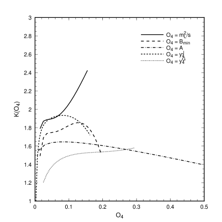
As defined before, the light hemisphere mass is the smaller invariant mass of the two hemispheres formed by separating the event by a plane normal to the thrust axis. The NLO coefficient CML2/ssubscript𝐶superscriptsubscript𝑀𝐿2𝑠C_{M_{L}^{2}/s} evaluted at the physical scale μ=s𝜇𝑠\mu=\sqrt{s} together with the LO term is given in Table 3. The errors are estimates from the numerical program and are typically 2-3% for each entry. As with the previously known results on four jet event shapes, the NLO terms are significantly larger than the LO term. Here, we see that CML2/ssubscript𝐶superscriptsubscript𝑀𝐿2𝑠C_{M_{L}^{2}/s} is typically 50 times larger than BML2/ssubscript𝐵superscriptsubscript𝑀𝐿2𝑠B_{M_{L}^{2}/s} so that even when the additional factor of αs/2πsubscript𝛼𝑠2𝜋\alpha_{s}/2\pi is restored, the NLO correction is large. This is illustrated in Fig. 1 where the K factor defined by,

KO4=1+(αs(s)2π)CO4BO4,subscript𝐾subscript𝑂41subscript𝛼𝑠𝑠2𝜋subscript𝐶subscript𝑂4subscript𝐵subscript𝑂4K_{O_{4}}=1+\left(\frac{\alpha_{s}(\sqrt{s})}{2\pi}\right)\frac{C_{O_{4}}}{B_{O_{4}}}, (4.1)

is shown for O4=ML2/ssubscript𝑂4superscriptsubscript𝑀𝐿2𝑠O_{4}=M_{L}^{2}/s. We see that the K factor increases with the value of the observable, rising from 1.8 at small ML2/ssuperscriptsubscript𝑀𝐿2𝑠M_{L}^{2}/s up to 2.4. This behaviour is similar to that observed for other four jet event shapes [11].
Refer to caption
Figure 1: The K-factors defined according to eq. (4.1) for four jet event shapes, the light hemisphere mass (solid), narrow jet broadening (long-dashed), Aplanarity (dot-dashed) and jet transition variables in the JADE (short-dashed) and Geneva (dotted) schemes. Each variable has a different kinematic range.

4.2 Narrow Hemisphere Broadening

Narrow hemisphere broadening, Bminsubscript𝐵minB_{\rm min}, is defined in a similiar manner to the light hemisphere mass. The event is again divided into two hemispheres by the plane normal to the thrust axis, but now the momenta transverse to the thrust axis is summed (normalised by the sum of absolute momenta) in each hemisphere. The narrow hemisphere is that with the least transverse momentum with respect to the thrust axis. Numerical results for this variable as calculated by EERAD2 can be found in Table 4. As with the light hemisphere mass, the NLO contribution is significant yielding a K factor of roughly 1.7 over most of the kinematic range of the variable (see Fig. 1).

Bminsubscript𝐵B_{\min} BBminsubscript𝐵subscript𝐵B_{B_{\min}} CBminsubscript𝐶subscript𝐵C_{B_{\min}}
0.0150 (1.19±0.01)103plus-or-minus1.190.01superscript103(1.19\pm 0.01)\cdot 10^{3} (3.41±0.07)104plus-or-minus3.410.07superscript104(3.41\pm 0.07)\cdot 10^{4}
0.0250 (7.04±0.06)102plus-or-minus7.040.06superscript102(7.04\pm 0.06)\cdot 10^{2} (2.56±0.02)104plus-or-minus2.560.02superscript104(2.56\pm 0.02)\cdot 10^{4}
0.0350 (4.80±0.02)102plus-or-minus4.800.02superscript102(4.80\pm 0.02)\cdot 10^{2} (1.92±0.04)104plus-or-minus1.920.04superscript104(1.92\pm 0.04)\cdot 10^{4}
0.0450 (3.39±0.02)102plus-or-minus3.390.02superscript102(3.39\pm 0.02)\cdot 10^{2} (1.41±0.02)104plus-or-minus1.410.02superscript104(1.41\pm 0.02)\cdot 10^{4}
0.0550 (2.49±0.02)102plus-or-minus2.490.02superscript102(2.49\pm 0.02)\cdot 10^{2} (1.07±0.02)104plus-or-minus1.070.02superscript104(1.07\pm 0.02)\cdot 10^{4}
0.0650 (1.89±0.02)102plus-or-minus1.890.02superscript102(1.89\pm 0.02)\cdot 10^{2} (8.04±0.12)103plus-or-minus8.040.12superscript103(8.04\pm 0.12)\cdot 10^{3}
0.0750 (1.43±0.02)102plus-or-minus1.430.02superscript102(1.43\pm 0.02)\cdot 10^{2} (6.29±0.12)103plus-or-minus6.290.12superscript103(6.29\pm 0.12)\cdot 10^{3}
0.0850 (1.08±0.01)102plus-or-minus1.080.01superscript102(1.08\pm 0.01)\cdot 10^{2} (4.81±0.08)103plus-or-minus4.810.08superscript103(4.81\pm 0.08)\cdot 10^{3}
0.0950 (8.19±0.04)101plus-or-minus8.190.04superscript101(8.19\pm 0.04)\cdot 10^{1} (3.65±0.08)103plus-or-minus3.650.08superscript103(3.65\pm 0.08)\cdot 10^{3}
0.1050 (6.23±0.08)101plus-or-minus6.230.08superscript101(6.23\pm 0.08)\cdot 10^{1} (2.77±0.09)103plus-or-minus2.770.09superscript103(2.77\pm 0.09)\cdot 10^{3}
0.1150 (4.69±0.06)101plus-or-minus4.690.06superscript101(4.69\pm 0.06)\cdot 10^{1} (2.10±0.04)103plus-or-minus2.100.04superscript103(2.10\pm 0.04)\cdot 10^{3}
0.1250 (3.37±0.04)101plus-or-minus3.370.04superscript101(3.37\pm 0.04)\cdot 10^{1} (1.45±0.04)103plus-or-minus1.450.04superscript103(1.45\pm 0.04)\cdot 10^{3}
0.1350 (2.36±0.04)101plus-or-minus2.360.04superscript101(2.36\pm 0.04)\cdot 10^{1} (1.09±0.03)103plus-or-minus1.090.03superscript103(1.09\pm 0.03)\cdot 10^{3}
0.1450 (1.64±0.03)101plus-or-minus1.640.03superscript101(1.64\pm 0.03)\cdot 10^{1} (7.07±0.25)102plus-or-minus7.070.25superscript102(7.07\pm 0.25)\cdot 10^{2}
0.1550 (9.82±0.12)100plus-or-minus9.820.12superscript100(9.82\pm 0.12)\cdot 10^{0} (4.48±0.15)102plus-or-minus4.480.15superscript102(4.48\pm 0.15)\cdot 10^{2}
0.1650 (5.08±0.12)100plus-or-minus5.080.12superscript100(5.08\pm 0.12)\cdot 10^{0} (2.18±0.10)102plus-or-minus2.180.10superscript102(2.18\pm 0.10)\cdot 10^{2}
0.1750 (1.71±0.04)100plus-or-minus1.710.04superscript100(1.71\pm 0.04)\cdot 10^{0} (7.53±0.33)101plus-or-minus7.530.33superscript101(7.53\pm 0.33)\cdot 10^{1}
0.1850 (4.32±0.11)101plus-or-minus4.320.11superscript101(4.32\pm 0.11)\cdot 10^{-1} (1.59±0.12)101plus-or-minus1.590.12superscript101(1.59\pm 0.12)\cdot 10^{1}
0.1950 (5.47±0.11)102plus-or-minus5.470.11superscript102(5.47\pm 0.11)\cdot 10^{-2} (1.34±0.24)100plus-or-minus1.340.24superscript100(1.34\pm 0.24)\cdot 10^{0}
Table 4: The leading and next-to-leading order coefficients for the narrow jet broadening Bminsubscript𝐵B_{\min}.

4.3 Aplanarity

As described earlier, Aplanarity is essentially the smallest eigenvalue of the quadratic momentum tensor. The NLO coefficient CAsubscript𝐶𝐴C_{A} evaluted at the physical scale μ=s𝜇𝑠\mu=\sqrt{s} together with the LO term is given in Table 5. Once again, the NLO terms are significantly larger than the LO term BAsubscript𝐵𝐴B_{A} and, as can be seen in Fig. 1 gives rise to K factor of roughly 1.5.

A𝐴A BAsubscript𝐵𝐴B_{A} CAsubscript𝐶𝐴C_{A}
0.0300 (7.25±0.04)101plus-or-minus7.250.04superscript101(7.25\pm 0.04)\cdot 10^{1} (2.48±0.10)103plus-or-minus2.480.10superscript103(2.48\pm 0.10)\cdot 10^{3}
0.0500 (3.87±0.03)101plus-or-minus3.870.03superscript101(3.87\pm 0.03)\cdot 10^{1} (1.40±0.07)103plus-or-minus1.400.07superscript103(1.40\pm 0.07)\cdot 10^{3}
0.0700 (2.35±0.02)101plus-or-minus2.350.02superscript101(2.35\pm 0.02)\cdot 10^{1} (7.65±0.58)102plus-or-minus7.650.58superscript102(7.65\pm 0.58)\cdot 10^{2}
0.0900 (1.57±0.02)101plus-or-minus1.570.02superscript101(1.57\pm 0.02)\cdot 10^{1} (5.55±0.40)102plus-or-minus5.550.40superscript102(5.55\pm 0.40)\cdot 10^{2}
0.1100 (1.06±0.01)101plus-or-minus1.060.01superscript101(1.06\pm 0.01)\cdot 10^{1} (4.07±0.36)102plus-or-minus4.070.36superscript102(4.07\pm 0.36)\cdot 10^{2}
0.1300 (7.45±0.12)100plus-or-minus7.450.12superscript100(7.45\pm 0.12)\cdot 10^{0} (2.34±0.34)102plus-or-minus2.340.34superscript102(2.34\pm 0.34)\cdot 10^{2}
0.1500 (5.19±0.07)100plus-or-minus5.190.07superscript100(5.19\pm 0.07)\cdot 10^{0} (1.75±0.20)102plus-or-minus1.750.20superscript102(1.75\pm 0.20)\cdot 10^{2}
0.1700 (3.76±0.08)100plus-or-minus3.760.08superscript100(3.76\pm 0.08)\cdot 10^{0} (1.23±0.28)102plus-or-minus1.230.28superscript102(1.23\pm 0.28)\cdot 10^{2}
0.1900 (2.68±0.04)100plus-or-minus2.680.04superscript100(2.68\pm 0.04)\cdot 10^{0} (9.42±1.25)101plus-or-minus9.421.25superscript101(9.42\pm 1.25)\cdot 10^{1}
0.2100 (2.02±0.03)100plus-or-minus2.020.03superscript100(2.02\pm 0.03)\cdot 10^{0} (6.37±0.98)101plus-or-minus6.370.98superscript101(6.37\pm 0.98)\cdot 10^{1}
0.2300 (1.32±0.02)100plus-or-minus1.320.02superscript100(1.32\pm 0.02)\cdot 10^{0} (4.19±0.99)101plus-or-minus4.190.99superscript101(4.19\pm 0.99)\cdot 10^{1}
0.2500 (9.70±0.16)101plus-or-minus9.700.16superscript101(9.70\pm 0.16)\cdot 10^{-1} (3.14±0.67)101plus-or-minus3.140.67superscript101(3.14\pm 0.67)\cdot 10^{1}
0.2700 (6.43±0.16)101plus-or-minus6.430.16superscript101(6.43\pm 0.16)\cdot 10^{-1} (2.08±0.45)101plus-or-minus2.080.45superscript101(2.08\pm 0.45)\cdot 10^{1}
0.2900 (4.28±0.14)101plus-or-minus4.280.14superscript101(4.28\pm 0.14)\cdot 10^{-1} (1.25±0.34)101plus-or-minus1.250.34superscript101(1.25\pm 0.34)\cdot 10^{1}
0.3100 (2.87±0.12)101plus-or-minus2.870.12superscript101(2.87\pm 0.12)\cdot 10^{-1} (7.58±1.36)100plus-or-minus7.581.36superscript100(7.58\pm 1.36)\cdot 10^{0}
0.3300 (1.79±0.03)101plus-or-minus1.790.03superscript101(1.79\pm 0.03)\cdot 10^{-1} (6.13±1.67)100plus-or-minus6.131.67superscript100(6.13\pm 1.67)\cdot 10^{0}
0.3500 (1.07±0.02)101plus-or-minus1.070.02superscript101(1.07\pm 0.02)\cdot 10^{-1} (3.94±0.91)100plus-or-minus3.940.91superscript100(3.94\pm 0.91)\cdot 10^{0}
0.3700 (6.66±0.20)102plus-or-minus6.660.20superscript102(6.66\pm 0.20)\cdot 10^{-2} (2.00±0.40)100plus-or-minus2.000.40superscript100(2.00\pm 0.40)\cdot 10^{0}
0.3900 (3.30±0.20)102plus-or-minus3.300.20superscript102(3.30\pm 0.20)\cdot 10^{-2} (9.26±3.71)101plus-or-minus9.263.71superscript101(9.26\pm 3.71)\cdot 10^{-1}
0.4100 (1.56±0.09)102plus-or-minus1.560.09superscript102(1.56\pm 0.09)\cdot 10^{-2} (4.00±1.52)101plus-or-minus4.001.52superscript101(4.00\pm 1.52)\cdot 10^{-1}
0.4300 (5.58±0.22)103plus-or-minus5.580.22superscript103(5.58\pm 0.22)\cdot 10^{-3} (1.50±0.92)101plus-or-minus1.500.92superscript101(1.50\pm 0.92)\cdot 10^{-1}
0.4500 (1.53±0.18)103plus-or-minus1.530.18superscript103(1.53\pm 0.18)\cdot 10^{-3} (7.44±3.27)102plus-or-minus7.443.27superscript102(7.44\pm 3.27)\cdot 10^{-2}
0.4700 (1.80±0.23)104plus-or-minus1.800.23superscript104(1.80\pm 0.23)\cdot 10^{-4} (1.76±7.87)103plus-or-minus1.767.87superscript103(1.76\pm 7.87)\cdot 10^{-3}
0.4900 (1.38±0.45)105plus-or-minus1.380.45superscript105(1.38\pm 0.45)\cdot 10^{-5} (9.93±54.90)105plus-or-minus9.9354.90superscript105(9.93\pm 54.90)\cdot 10^{-5}
Table 5: The leading and next-to-leading order coefficients for Aplanarity.

4.4 Jet transition variables

As previously stated the jet transition variable y4Ssuperscriptsubscript𝑦4𝑆y_{4}^{S} describes the scale where two jets merge, thereby changing a four jet event into a three jet event. This is essentially the same as the derivative of the four jet rate with respect to the jet resolution parameter ycutsubscript𝑦cuty_{\rm cut}. However, the number of jets in an event is dependent on the jet finding algorithm used to define the ‘closeness’ of particles which is compared with ycutsubscript𝑦cuty_{\rm cut}. In [11] the transition rate for the the Durham jet finding algorithm [28] is given and we have checked that our results are consistent with these predictions. Here, we provide results for two other jet algorithms, the JADE and Geneva [29] schemes for which the jet finding measures are given in eq. (2.9). We note that the Geneva algorithm enjoys the same benefits as the Durham algorithm in that it is also supposed to exponentiate, enabling infrared logarithms to be safely resummed. It also ensures that softly radiated gluons are clustered with hard partons unless the angle of separation between two soft gluons is much smaller than the angular separation between them and a hard parton.

Our results for the two schemes are given in Tables 6 and 7. As can be seen from the tables the NLO coefficients are large, which is again reflected in the large corrections shown in Fig. 1. The K factor for the JADE scheme is roughly 1.8-1.9, but is slightly smaller for the Geneva algorithm, typically in the region 1.4-1.6.

y4Gsuperscriptsubscript𝑦4𝐺y_{4}^{G} By4Gsubscript𝐵superscriptsubscript𝑦4𝐺B_{y_{4}^{G}} Cy4Gsubscript𝐶superscriptsubscript𝑦4𝐺C_{y_{4}^{G}}
0.0250 (8.00±0.04)102plus-or-minus8.000.04superscript102(8.00\pm 0.04)\cdot 10^{2} (9.93±0.34)103plus-or-minus9.930.34superscript103(9.93\pm 0.34)\cdot 10^{3}
0.0350 (5.59±0.04)102plus-or-minus5.590.04superscript102(5.59\pm 0.04)\cdot 10^{2} (9.91±0.30)103plus-or-minus9.910.30superscript103(9.91\pm 0.30)\cdot 10^{3}
0.0450 (4.15±0.03)102plus-or-minus4.150.03superscript102(4.15\pm 0.03)\cdot 10^{2} (8.57±0.13)103plus-or-minus8.570.13superscript103(8.57\pm 0.13)\cdot 10^{3}
0.0550 (3.15±0.03)102plus-or-minus3.150.03superscript102(3.15\pm 0.03)\cdot 10^{2} (7.31±0.18)103plus-or-minus7.310.18superscript103(7.31\pm 0.18)\cdot 10^{3}
0.0650 (2.47±0.02)102plus-or-minus2.470.02superscript102(2.47\pm 0.02)\cdot 10^{2} (5.96±0.12)103plus-or-minus5.960.12superscript103(5.96\pm 0.12)\cdot 10^{3}
0.0750 (1.93±0.02)102plus-or-minus1.930.02superscript102(1.93\pm 0.02)\cdot 10^{2} (4.99±0.14)103plus-or-minus4.990.14superscript103(4.99\pm 0.14)\cdot 10^{3}
0.0850 (1.50±0.02)102plus-or-minus1.500.02superscript102(1.50\pm 0.02)\cdot 10^{2} (3.96±0.11)103plus-or-minus3.960.11superscript103(3.96\pm 0.11)\cdot 10^{3}
0.0950 (1.23±0.01)102plus-or-minus1.230.01superscript102(1.23\pm 0.01)\cdot 10^{2} (3.36±0.13)103plus-or-minus3.360.13superscript103(3.36\pm 0.13)\cdot 10^{3}
0.1050 (9.88±0.12)101plus-or-minus9.880.12superscript101(9.88\pm 0.12)\cdot 10^{1} (2.84±0.06)103plus-or-minus2.840.06superscript103(2.84\pm 0.06)\cdot 10^{3}
0.1150 (7.90±0.09)101plus-or-minus7.900.09superscript101(7.90\pm 0.09)\cdot 10^{1} (2.19±0.09)103plus-or-minus2.190.09superscript103(2.19\pm 0.09)\cdot 10^{3}
0.1250 (6.07±0.08)101plus-or-minus6.070.08superscript101(6.07\pm 0.08)\cdot 10^{1} (1.69±0.11)103plus-or-minus1.690.11superscript103(1.69\pm 0.11)\cdot 10^{3}
0.1350 (4.79±0.07)101plus-or-minus4.790.07superscript101(4.79\pm 0.07)\cdot 10^{1} (1.53±0.08)103plus-or-minus1.530.08superscript103(1.53\pm 0.08)\cdot 10^{3}
0.1450 (3.84±0.06)101plus-or-minus3.840.06superscript101(3.84\pm 0.06)\cdot 10^{1} (1.15±0.04)103plus-or-minus1.150.04superscript103(1.15\pm 0.04)\cdot 10^{3}
0.1550 (3.00±0.05)101plus-or-minus3.000.05superscript101(3.00\pm 0.05)\cdot 10^{1} (8.41±0.53)102plus-or-minus8.410.53superscript102(8.41\pm 0.53)\cdot 10^{2}
0.1650 (2.26±0.04)101plus-or-minus2.260.04superscript101(2.26\pm 0.04)\cdot 10^{1} (6.52±0.36)102plus-or-minus6.520.36superscript102(6.52\pm 0.36)\cdot 10^{2}
0.1750 (1.61±0.02)101plus-or-minus1.610.02superscript101(1.61\pm 0.02)\cdot 10^{1} (4.99±0.33)102plus-or-minus4.990.33superscript102(4.99\pm 0.33)\cdot 10^{2}
0.1850 (1.21±0.02)101plus-or-minus1.210.02superscript101(1.21\pm 0.02)\cdot 10^{1} (3.60±0.23)102plus-or-minus3.600.23superscript102(3.60\pm 0.23)\cdot 10^{2}
0.1950 (8.71±0.27)100plus-or-minus8.710.27superscript100(8.71\pm 0.27)\cdot 10^{0} (2.53±0.20)102plus-or-minus2.530.20superscript102(2.53\pm 0.20)\cdot 10^{2}
0.2050 (5.70±0.16)100plus-or-minus5.700.16superscript100(5.70\pm 0.16)\cdot 10^{0} (1.78±0.17)102plus-or-minus1.780.17superscript102(1.78\pm 0.17)\cdot 10^{2}
0.2150 (3.89±0.09)100plus-or-minus3.890.09superscript100(3.89\pm 0.09)\cdot 10^{0} (1.20±0.11)102plus-or-minus1.200.11superscript102(1.20\pm 0.11)\cdot 10^{2}
0.2250 (2.41±0.06)100plus-or-minus2.410.06superscript100(2.41\pm 0.06)\cdot 10^{0} (6.83±0.87)101plus-or-minus6.830.87superscript101(6.83\pm 0.87)\cdot 10^{1}
0.2350 (1.43±0.05)100plus-or-minus1.430.05superscript100(1.43\pm 0.05)\cdot 10^{0} (4.87±0.36)101plus-or-minus4.870.36superscript101(4.87\pm 0.36)\cdot 10^{1}
0.2450 (7.69±0.30)101plus-or-minus7.690.30superscript101(7.69\pm 0.30)\cdot 10^{-1} (2.57±0.25)101plus-or-minus2.570.25superscript101(2.57\pm 0.25)\cdot 10^{1}
0.2550 (3.78±0.09)101plus-or-minus3.780.09superscript101(3.78\pm 0.09)\cdot 10^{-1} (1.18±0.13)101plus-or-minus1.180.13superscript101(1.18\pm 0.13)\cdot 10^{1}
0.2650 (1.50±0.04)101plus-or-minus1.500.04superscript101(1.50\pm 0.04)\cdot 10^{-1} (4.57±0.79)100plus-or-minus4.570.79superscript100(4.57\pm 0.79)\cdot 10^{0}
0.2750 (4.20±0.17)102plus-or-minus4.200.17superscript102(4.20\pm 0.17)\cdot 10^{-2} (1.15±0.35)100plus-or-minus1.150.35superscript100(1.15\pm 0.35)\cdot 10^{0}
0.2850 (4.59±0.39)103plus-or-minus4.590.39superscript103(4.59\pm 0.39)\cdot 10^{-3} (1.16±0.65)101plus-or-minus1.160.65superscript101(1.16\pm 0.65)\cdot 10^{-1}
0.2950 (5.37±0.91)105plus-or-minus5.370.91superscript105(5.37\pm 0.91)\cdot 10^{-5} (2.15±1.11)103plus-or-minus2.151.11superscript103(2.15\pm 1.11)\cdot 10^{-3}
Table 6: The leading and next-to-leading order coefficients for the jet transition variable in the Geneva-E algorithm y4Gsuperscriptsubscript𝑦4𝐺y_{4}^{G}.
y4Jsuperscriptsubscript𝑦4𝐽y_{4}^{J} By4Jsubscript𝐵superscriptsubscript𝑦4𝐽B_{y_{4}^{J}} Cy4Jsubscript𝐶superscriptsubscript𝑦4𝐽C_{y_{4}^{J}}
0.0075 (6.02±0.01)102plus-or-minus6.020.01superscript102(6.02\pm 0.01)\cdot 10^{2} (1.75±0.01)104plus-or-minus1.750.01superscript104(1.75\pm 0.01)\cdot 10^{4}
0.0125 (3.60±0.01)102plus-or-minus3.600.01superscript102(3.60\pm 0.01)\cdot 10^{2} (1.33±0.02)104plus-or-minus1.330.02superscript104(1.33\pm 0.02)\cdot 10^{4}
0.0175 (2.47±0.01)102plus-or-minus2.470.01superscript102(2.47\pm 0.01)\cdot 10^{2} (1.02±0.04)104plus-or-minus1.020.04superscript104(1.02\pm 0.04)\cdot 10^{4}
0.0225 (1.78±0.01)102plus-or-minus1.780.01superscript102(1.78\pm 0.01)\cdot 10^{2} (7.63±0.32)103plus-or-minus7.630.32superscript103(7.63\pm 0.32)\cdot 10^{3}
0.0275 (1.34±0.01)102plus-or-minus1.340.01superscript102(1.34\pm 0.01)\cdot 10^{2} (6.19±0.16)103plus-or-minus6.190.16superscript103(6.19\pm 0.16)\cdot 10^{3}
0.0325 (1.01±0.01)102plus-or-minus1.010.01superscript102(1.01\pm 0.01)\cdot 10^{2} (4.76±0.12)103plus-or-minus4.760.12superscript103(4.76\pm 0.12)\cdot 10^{3}
0.0375 (7.88±0.08)101plus-or-minus7.880.08superscript101(7.88\pm 0.08)\cdot 10^{1} (3.86±0.11)103plus-or-minus3.860.11superscript103(3.86\pm 0.11)\cdot 10^{3}
0.0425 (6.19±0.05)101plus-or-minus6.190.05superscript101(6.19\pm 0.05)\cdot 10^{1} (3.07±0.16)103plus-or-minus3.070.16superscript103(3.07\pm 0.16)\cdot 10^{3}
0.0475 (4.99±0.05)101plus-or-minus4.990.05superscript101(4.99\pm 0.05)\cdot 10^{1} (2.38±0.12)103plus-or-minus2.380.12superscript103(2.38\pm 0.12)\cdot 10^{3}
0.0525 (3.89±0.05)101plus-or-minus3.890.05superscript101(3.89\pm 0.05)\cdot 10^{1} (2.08±0.11)103plus-or-minus2.080.11superscript103(2.08\pm 0.11)\cdot 10^{3}
0.0575 (3.13±0.05)101plus-or-minus3.130.05superscript101(3.13\pm 0.05)\cdot 10^{1} (1.54±0.05)103plus-or-minus1.540.05superscript103(1.54\pm 0.05)\cdot 10^{3}
0.0625 (2.43±0.04)101plus-or-minus2.430.04superscript101(2.43\pm 0.04)\cdot 10^{1} (1.26±0.03)103plus-or-minus1.260.03superscript103(1.26\pm 0.03)\cdot 10^{3}
0.0675 (1.90±0.03)101plus-or-minus1.900.03superscript101(1.90\pm 0.03)\cdot 10^{1} (9.68±0.58)102plus-or-minus9.680.58superscript102(9.68\pm 0.58)\cdot 10^{2}
0.0725 (1.49±0.04)101plus-or-minus1.490.04superscript101(1.49\pm 0.04)\cdot 10^{1} (7.70±0.35)102plus-or-minus7.700.35superscript102(7.70\pm 0.35)\cdot 10^{2}
0.0775 (1.21±0.02)101plus-or-minus1.210.02superscript101(1.21\pm 0.02)\cdot 10^{1} (5.89±0.41)102plus-or-minus5.890.41superscript102(5.89\pm 0.41)\cdot 10^{2}
0.0825 (9.38±0.18)100plus-or-minus9.380.18superscript100(9.38\pm 0.18)\cdot 10^{0} (4.83±0.35)102plus-or-minus4.830.35superscript102(4.83\pm 0.35)\cdot 10^{2}
0.0875 (6.94±0.09)100plus-or-minus6.940.09superscript100(6.94\pm 0.09)\cdot 10^{0} (3.50±0.19)102plus-or-minus3.500.19superscript102(3.50\pm 0.19)\cdot 10^{2}
0.0925 (5.36±0.11)100plus-or-minus5.360.11superscript100(5.36\pm 0.11)\cdot 10^{0} (2.48±0.27)102plus-or-minus2.480.27superscript102(2.48\pm 0.27)\cdot 10^{2}
0.0975 (3.85±0.06)100plus-or-minus3.850.06superscript100(3.85\pm 0.06)\cdot 10^{0} (1.93±0.19)102plus-or-minus1.930.19superscript102(1.93\pm 0.19)\cdot 10^{2}
0.1025 (2.84±0.07)100plus-or-minus2.840.07superscript100(2.84\pm 0.07)\cdot 10^{0} (1.26±0.11)102plus-or-minus1.260.11superscript102(1.26\pm 0.11)\cdot 10^{2}
0.1075 (1.97±0.07)100plus-or-minus1.970.07superscript100(1.97\pm 0.07)\cdot 10^{0} (9.99±1.22)101plus-or-minus9.991.22superscript101(9.99\pm 1.22)\cdot 10^{1}
0.1125 (1.30±0.06)100plus-or-minus1.300.06superscript100(1.30\pm 0.06)\cdot 10^{0} (6.69±0.94)101plus-or-minus6.690.94superscript101(6.69\pm 0.94)\cdot 10^{1}
0.1175 (8.32±0.37)101plus-or-minus8.320.37superscript101(8.32\pm 0.37)\cdot 10^{-1} (3.57±0.52)101plus-or-minus3.570.52superscript101(3.57\pm 0.52)\cdot 10^{1}
0.1225 (4.94±0.07)101plus-or-minus4.940.07superscript101(4.94\pm 0.07)\cdot 10^{-1} (2.36±0.44)101plus-or-minus2.360.44superscript101(2.36\pm 0.44)\cdot 10^{1}
0.1275 (3.05±0.10)101plus-or-minus3.050.10superscript101(3.05\pm 0.10)\cdot 10^{-1} (1.85±0.38)101plus-or-minus1.850.38superscript101(1.85\pm 0.38)\cdot 10^{1}
0.1325 (1.70±0.03)101plus-or-minus1.700.03superscript101(1.70\pm 0.03)\cdot 10^{-1} (8.38±3.15)100plus-or-minus8.383.15superscript100(8.38\pm 3.15)\cdot 10^{0}
0.1375 (8.94±0.29)102plus-or-minus8.940.29superscript102(8.94\pm 0.29)\cdot 10^{-2} (4.99±1.15)100plus-or-minus4.991.15superscript100(4.99\pm 1.15)\cdot 10^{0}
0.1425 (4.20±0.12)102plus-or-minus4.200.12superscript102(4.20\pm 0.12)\cdot 10^{-2} (2.01±0.38)100plus-or-minus2.010.38superscript100(2.01\pm 0.38)\cdot 10^{0}
0.1475 (1.67±0.07)102plus-or-minus1.670.07superscript102(1.67\pm 0.07)\cdot 10^{-2} (1.08±0.73)100plus-or-minus1.080.73superscript100(1.08\pm 0.73)\cdot 10^{0}
0.1525 (5.51±0.44)103plus-or-minus5.510.44superscript103(5.51\pm 0.44)\cdot 10^{-3} (3.94±2.32)101plus-or-minus3.942.32superscript101(3.94\pm 2.32)\cdot 10^{-1}
0.1575 (8.48±0.58)104plus-or-minus8.480.58superscript104(8.48\pm 0.58)\cdot 10^{-4} (4.37±2.44)102plus-or-minus4.372.44superscript102(4.37\pm 2.44)\cdot 10^{-2}
Table 7: The leading and next-to-leading order coefficients for the jet transition variable in the JADE-E0 algorithm y4Jsuperscriptsubscript𝑦4𝐽y_{4}^{J}.

5 Comparison with experimental data

Four jet event shape observables have been studied extensively by the four LEP experiments. However, the most complete analysis of event shape variables has been carried out by the DELPHI collaboration [33]. Here, they study all of the event shape variables discussed in section 2. Distributions based on charged particles alone as well as charged and neutral particles are presented. In this section, we wish to examine whether or not these event shapes can be described by fixed order perturbation theory. As discussed earlier, to avoid numerical instabilities in the infrared region where fixed order perturbation theory is no longer valid we impose a cut on the smallness of the variable that is generally equal to the lower edge of the second bin. More precisely, that is,

D𝐷\displaystyle D >\displaystyle> 0.008,0.008\displaystyle 0.008,
Tminorsubscript𝑇minor\displaystyle T_{\rm minor} >\displaystyle> 0.02,0.02\displaystyle 0.02,
ML2/ssuperscriptsubscript𝑀𝐿2𝑠\displaystyle M_{L}^{2}/s >\displaystyle> 0.01,0.01\displaystyle 0.01,
Bminsubscript𝐵\displaystyle B_{\min} >\displaystyle> 0.01,0.01\displaystyle 0.01,
A𝐴\displaystyle A >\displaystyle> 0.005,0.005\displaystyle 0.005,
y4Dsuperscriptsubscript𝑦4𝐷\displaystyle y_{4}^{D} >\displaystyle> 0.002,0.002\displaystyle 0.002,
y4Jsuperscriptsubscript𝑦4𝐽\displaystyle y_{4}^{J} >\displaystyle> 0.002.0.002\displaystyle 0.002. (5.1)

The experimental distributions are normalised to the hadronic cross section (rather than the Born cross section) and are also not weighted by the observable, but are rather,

1σhaddσdO4=(αs(μ)2π)2BO4O4+(αs(μ)2π)3(2β0log(μ2s)BO4O4+CO42BO4O4).1subscript𝜎had𝑑𝜎𝑑subscript𝑂4superscriptsubscript𝛼𝑠𝜇2𝜋2subscript𝐵subscript𝑂4subscript𝑂4superscriptsubscript𝛼𝑠𝜇2𝜋32subscript𝛽0superscript𝜇2𝑠subscript𝐵subscript𝑂4subscript𝑂4subscript𝐶subscript𝑂42subscript𝐵subscript𝑂4subscript𝑂4\frac{1}{\sigma_{\rm had}}\cdot\,\frac{d\sigma}{dO_{4}}=\left(\frac{\alpha_{s}(\mu)}{2\pi}\right)^{2}\frac{B_{O_{4}}}{O_{4}}+\left(\frac{\alpha_{s}(\mu)}{2\pi}\right)^{3}\left(2\beta_{0}\log\left(\frac{\mu^{2}}{s}\right)\frac{B_{O_{4}}}{O_{4}}+\frac{C_{O_{4}}-2B_{O_{4}}}{O_{4}}\right). (5.2)

Throughout, we choose αs(MZ)=0.118subscript𝛼𝑠subscript𝑀𝑍0.118\alpha_{s}(M_{Z})=0.118 which is consistent with the current world average [34]. In each case, the theoretical predictions have been evaluated using bins of the same size as in the experiment and therefore appear as histograms in the plots. The data is corrected for detector effects, but not for hadronisation effects.

(a) Refer to caption (b) Refer to caption
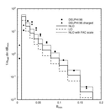
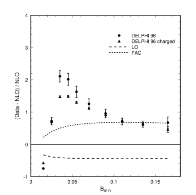
Figure 2: The leading order (dashed) and next-to-leading order (solid) predictions evaluated at the physical scale μ=s=MZ𝜇𝑠subscript𝑀𝑍\mu=\sqrt{s}=M_{Z} for (a) 1/σhaddσ/dBmin1subscript𝜎had𝑑𝜎𝑑subscript𝐵min1/\sigma_{\rm had}\cdot d\sigma/dB_{\rm min} compared to the published DELPHI data [33] and (b) the difference between data and NLO theory (normalised to NLO). The short-dashed line shows the next-to-leading order prediction using the FAC scale (see eq. (2.12)).

(a) Refer to caption (b) Refer to caption

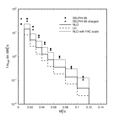
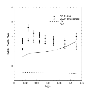
Figure 3: The leading order (dashed) and next-to-leading order (solid) predictions evaluated at the physical scale μ=s=MZ𝜇𝑠subscript𝑀𝑍\mu=\sqrt{s}=M_{Z} for (a) 1/σhaddσ/d(ML2/s)1subscript𝜎had𝑑𝜎𝑑superscriptsubscript𝑀𝐿2𝑠1/\sigma_{\rm had}\cdot d\sigma/d(M_{L}^{2}/s) compared to the published DELPHI data [33] and (b) the difference between data and NLO theory (normalised to NLO). The short-dashed line shows the next-to-leading order prediction using the FAC scale (see eq. (2.12)).

(a) Refer to caption (b) Refer to caption

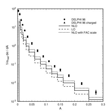
Figure 4: The leading order (dashed) and next-to-leading order (solid) predictions evaluated at the physical scale μ=s=MZ𝜇𝑠subscript𝑀𝑍\mu=\sqrt{s}=M_{Z} for (a) 1/σhaddσ/dA1subscript𝜎had𝑑𝜎𝑑𝐴1/\sigma_{\rm had}\cdot d\sigma/dA compared to the published DELPHI data [33] and (b) the difference between data and NLO theory (normalised to NLO). The short-dashed line shows the next-to-leading order prediction using the FAC scale (see eq. (2.12)).

Figs. 2, 3 and 4 show the comparison between the leading order and next-to-leading order predictions evaluated at the physical scale μ=s=MZ𝜇𝑠subscript𝑀𝑍\mu=\sqrt{s}=M_{Z} for narrow jet broadening, light hemisphere mass and Aplanarity with the published DELPHI data [33]. We see that in all three cases, the LO prediction undershoots the data by a significant factor (about a factor of four), and that including the NLO correction improves the situation but still gives a rate that is much lower than the data. However, the NLO prediction still contains a large renormalisation scale uncertainty. Usually, one varies the choice of scale about the physical scale by a factor of two or so, but as discussed earlier, the FAC scale defined in eq. (2.12) is an attractive alternative choice in that the known ultraviolet logarithms are resummed [35]. For both of these variables, the FAC scale is significantly less than the physical scale, for example, for Bminsubscript𝐵minB_{\rm min} , μFAC0.06ssimilar-tosuperscript𝜇𝐹𝐴𝐶0.06𝑠\mu^{FAC}\sim 0.06\sqrt{s}. This has the effect of increasing αssubscript𝛼𝑠\alpha_{s}, thereby increasing the NLO prediction and in both cases, we see much improved agreement at larger values of the observable. At smaller values, and particularly in the region where the data turns over the agreement is still poor. This, of course, is where the infrared logarithms are large and need to be resummed. Furthermore, we also expect non-perturbative hadronisation effects or power corrections to influence the perturbative shape of the distribution we have been concerned with [36, 37]. These contributions (together with resummation of the infrared logarithms) have played an important role in extracting useful information from analyses of three jet shape variables, and are likely to be important in analysing four jet event shapes.

(a) Refer to caption (b) Refer to caption
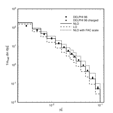
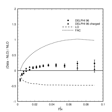
Figure 5: The leading order (dashed) and next-to-leading order (solid) predictions evaluated at the physical scale μ=s=MZ𝜇𝑠subscript𝑀𝑍\mu=\sqrt{s}=M_{Z} for (a) 1/σhaddσ/dy4J1subscript𝜎had𝑑𝜎𝑑superscriptsubscript𝑦4𝐽1/\sigma_{\rm had}\cdot d\sigma/dy_{4}^{J} compared to the published DELPHI data [33] and (b) the difference between data and NLO theory (normalised to NLO). The short-dashed line shows the next-to-leading order prediction using the FAC scale (see eq. (2.12)).

(a) Refer to caption (b) Refer to caption

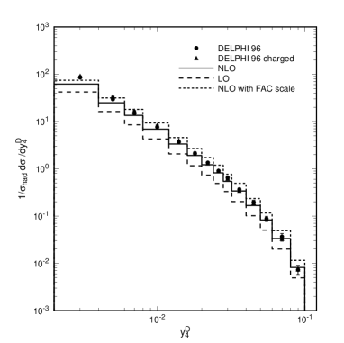
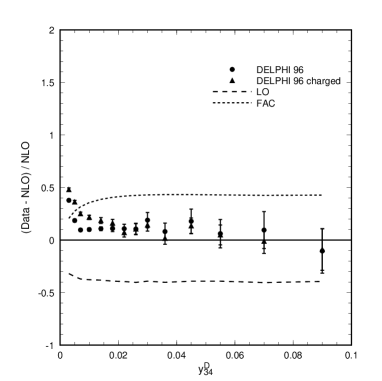
Figure 6: The leading order (dashed) and next-to-leading order (solid) predictions evaluated at the physical scale μ=s=MZ𝜇𝑠subscript𝑀𝑍\mu=\sqrt{s}=M_{Z} for (a) 1/σhaddσ/dy4D1subscript𝜎had𝑑𝜎𝑑superscriptsubscript𝑦4𝐷1/\sigma_{\rm had}\cdot d\sigma/dy_{4}^{D} compared to the published DELPHI data [33] and (b) the difference between data and NLO theory (normalised to NLO). The short-dashed line shows the next-to-leading order prediction using the FAC scale (see eq. (2.12)).

A similar comparison of the perturbative predictions for the jet transition rates with the DELPHI measurements444The DELPHI data gives the differential jet rate rather than the jet transition variable. Up to a small (similar-to\sim few %) correction from five (and more) jet events falling into a four jet configuration, the two quantities coincide at fixed order. is made in Figs. 5 and 6. Once again, the LO distribution lies well below the data. This time, the NLO prediction lies much closer to the data for most of the available kinematic range. The FAC scale rate usually lies above the NLO prediction so that the data lies within the range of uncertainty engendered by the renormalisation group.

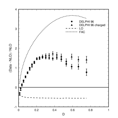
For completeness, Figs. 7 and 8 show the DELPHI data and perturbative predictions for the D𝐷D parameter and Tminorsubscript𝑇minorT_{\rm minor} repectively. As expected from the analysis of Nagy and Trócsányi [11], the LO prediction for D𝐷D is too low by a factor of about four, while at the physical scale μ=s=MZ𝜇𝑠subscript𝑀𝑍\mu=\sqrt{s}=M_{Z} the NLO distribution is roughly twice as large but still lies a factor of two below the data. However, for the FAC scale (which for the D𝐷D parameter is approximately 0.035s0.035𝑠0.035\sqrt{s}) the prediction overshoots by 50% or so for D>0.1𝐷0.1D>0.1 where the fixed order prediction is least affected by large infrared logs.

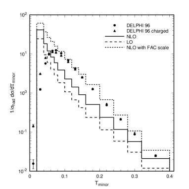
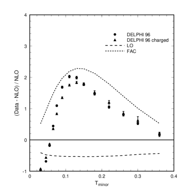
The importance of resumming these logs is clearly shown in Fig. 8 where the Tminorsubscript𝑇minorT_{\rm minor} distribution is shown. For Tminor>0.1subscript𝑇minor0.1T_{\rm minor}>0.1 the data again lies between the next-to-leading order predictions at the physical and FAC scales (which encompass an uncertainty of about a factor of almost three for Tminor0.2similar-tosubscript𝑇minor0.2T_{\rm minor}\sim 0.2). However, the turn-over at Tminor=0.1subscript𝑇minor0.1T_{\rm minor}=0.1 cannot be modelled without resumming the large logs which cause the perturbative prediction to grow rapidly. The same is true at small values of the light hemisphere mass and narrow jet broadening although there the effects are less pronounced because of the choice of bin sizes.

(a) Refer to caption (b) Refer to caption
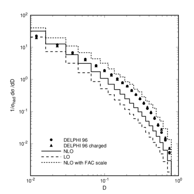
Figure 7: The leading order (dashed) and next-to-leading order (solid) predictions evaluated at the physical scale μ=s=MZ𝜇𝑠subscript𝑀𝑍\mu=\sqrt{s}=M_{Z} for (a) 1/σhaddσ/dD1subscript𝜎had𝑑𝜎𝑑𝐷1/\sigma_{\rm had}\cdot d\sigma/dD compared to the published DELPHI data [33] and (b) the difference between data and NLO theory (normalised to NLO). The short-dashed line shows the next-to-leading order prediction using the FAC scale (see eq. (2.12)).

(a) Refer to caption (b) Refer to caption

Figure 8: The leading order (dashed) and next-to-leading order (solid) predictions evaluated at the physical scale μ=s=MZ𝜇𝑠subscript𝑀𝑍\mu=\sqrt{s}=M_{Z} for (a) 1/σhaddσ/dTminor1subscript𝜎had𝑑𝜎𝑑subscript𝑇minor1/\sigma_{\rm had}\cdot d\sigma/dT_{\rm minor} compared to the published DELPHI data [33] and (b) the difference between data and NLO theory (normalised to NLO). The short-dashed line shows the next-to-leading order prediction using the FAC scale (see eq. (2.12)).

6 Conclusions

In this paper we have introduced a new Monte Carlo program for the calculation of 4 jet like observables in electron-positron annihilation. This program, EERAD2, is based on the known squared matrix elements for γ4superscript𝛾4\gamma^{*}\to 4 and 5 partons and numerically implements the necessary cancellations between the different final states using a hybrid of the commonly used subtraction and slicing schemes. This infrared cancellation scheme is detailed in the appendix.

We have checked that the numerical results obtained with EERAD2 are consistent with the two other available four jet programs MENLO PARC and DEBRECEN by recalculating the distributions for some of the previously determined four jet event variables (such as the D𝐷D parameter, thrust minor and the jet transition rate for the Durham jet algorithm) as well as the four jet rate. Within the (estimated) statistical Monte Carlo errors, there is excellent agreement.

We have also presented the leading and next-to-leading order scale independent coefficients for some previously uncalculated observables; the light hemisphere mass, narrow jet broadening, Aplanarity and the four jet transition variables with respect to the JADE and Geneva jet finding algorithms. For each of these observables, the next-to-leading order corrections calculated at the physical scale significantly increase the rate compared to leading order (see fig. 1). The renormalisation scale dependence is also rather large.

Furthermore, for each of these observables, we have made a comparison with the published data collected at LEP 1 energies by the DELPHI collaboration. With the exception of the y4subscript𝑦4y_{4} distributions, the data lies well above the NLO prediction, apart from in the infrared region where the NLO prediction grows rapidly (and where resummation of large logarithms is essential). Using the FAC scale, which is of the order of 0.10.10.1111% of the physical scale, increases the predicted rate and in general produces a slightly better agreement with the data. Taking together the size of the NLO corrections, the renormalisation scale dependence and poor agreement with data it appears that the inclusion of even higher order corrections and/or power corrections will be necessary to extract any useful information from these observations.

Although at first sight this may seem discouraging, it is instructive to compare this situation with the well-established results for the 3 jet-like variable 1Thrust1Thrust1-{\rm Thrust}. In this case, the next-to-leading order coefficient is also large compared to the leading order term, resulting in a K factor at the physical scale which varies from 1.41.41.41.61.61.6 throughout most of the kinematic range of the variable. These values are very similar to the case for the four jet observables that we have already discussed. In addition, it is also possible to compare the pure perturbative prediction for 1Thrust1Thrust1-{\rm Thrust} with the DELPHI data, as we have done for the four jet variables in section 4. This yields results which are qualitatively very similar to those shown for the D𝐷D-parameter and Tminorsubscript𝑇minorT_{\rm minor} in Figs. 7 and 8. In these cases, it is clear that the perturbative prediction – either at the physical scale or using the FAC choice – is insufficient to describe the data. However, after resummation of large logarithms and the inclusion of non-perturbative power corrections proportional to the inverse of the energy scale of the process, 1/Q1𝑄1/Q, it is known that the data for 1Thrust1Thrust1-{\rm Thrust} can be described very well [37]. In fact the thrust distribution forms a text-book example of how to interpret hadronic final states within QCD.

From this we conclude that discarding four jet-like event shape variables as unreliable at next-to-leading order is premature without proper consideration of the types of non-perturbative terms that have been successfully included for a variety of three jet-like observables. In this we disagree with the conclusions of reference [11].

In addition to these correction terms, all of the distributions that we have considered exhibit the infrared logarithmic behaviour (as the observable tends to zero) that is inevitable in a fixed order calculation. These logarithms are present in the coefficients BO4subscript𝐵subscript𝑂4B_{O_{4}} and CO4subscript𝐶subscript𝑂4C_{O_{4}} and can be parametrized in the form shown in eq. (2.13). By performing a fit to the distributions at low enough values of the variable O4subscript𝑂4O_{4} one should be able to extract the values of the coefficents Anmsubscript𝐴𝑛𝑚A_{nm} and, where possible, perform exponentiation to resum the infrared logarithms.

Acknowledgements

We thank Walter Giele for useful and stimulating discussions. We also thank Siggi Bethke for pointing out that the JADE-E0 jet algorithm does not use the E0 recombination scheme. JMC and MC thank the UK Particle Physics and Astronomy Research Council for research studentships. EWNG thanks the theory groups at CERN and Fermilab for their kind hospitality during the early stages of this work. This work was supported in part by the EU Fourth Framework Programme ‘Training and Mobility of Researchers’, Network ‘Quantum Chromodynamics and the Deep Structure of Elementary Particles’, contract FMRX-CT98-0194 (DG-12 - MIHT).

Appendix A Cancellation of infrared singularities

In order to compute next-to-leading order quantities in perturbation theory, it is necessary to combine the contribution from n𝑛n-parton one-loop Feynman diagrams with the (n+1)𝑛1(n+1)-parton bremstrahlung process. The virtual matrix elements are divergent and contain both infrared and ultraviolet singularities. The ultraviolet poles are removed by renormalisation, however the soft and collinear infrared poles are only cancelled when the virtual graphs are combined with the bremstrahlung process. Although the cancellation of infrared poles can be done analytically for simple processes, for complicated processes, it is necessary to resort to numerical techniques.

A.1 A simple example

The numerical problem has been nicely formulated by Kunszt and Soper [38] by means of a simple example integral,

=limϵ0{01dxxxϵF(x)1ϵF(0)},subscriptitalic-ϵ0subscriptsuperscript10𝑑𝑥𝑥superscript𝑥italic-ϵ𝐹𝑥1italic-ϵ𝐹0{\cal I}=\lim_{\epsilon\to 0}\left\{\int^{1}_{0}\frac{dx}{x}x^{\epsilon}F(x)-\frac{1}{\epsilon}F(0)\right\}, (A.1)

where F(x)𝐹𝑥F(x) is a known but complicated function representing the (n+1)𝑛1(n+1)-parton bremstrahlung matrix elements. Here x𝑥x represents the angle between two partons or the energy of a gluon and the integral over x𝑥x represents the additional phase space of the extra parton. As x0𝑥0x\to 0, the integrand is regularised by the xϵsuperscript𝑥italic-ϵx^{\epsilon} factor as in dimensional regularisation, however, the first term is still divergent as ϵ0italic-ϵ0\epsilon\to 0. This divergence is cancelled by the second term - the n𝑛n-parton one-loop contribution - so that the integral is finite. A variety of methods to compute {\cal I} have been developed.

The method used by Ellis, Ross and Terrano [1] is also known as the subtraction method. Here, a divergent term is subtracted from the first term and added to the second,

\displaystyle{\cal I} =\displaystyle= limϵ0{01dxxxϵ(F(x)F(0))+F(0)01dxxxϵ1ϵF(0)}subscriptitalic-ϵ0subscriptsuperscript10𝑑𝑥𝑥superscript𝑥italic-ϵ𝐹𝑥𝐹0𝐹0subscriptsuperscript10𝑑𝑥𝑥superscript𝑥italic-ϵ1italic-ϵ𝐹0\displaystyle\lim_{\epsilon\to 0}\left\{\int^{1}_{0}\frac{dx}{x}x^{\epsilon}(F(x)-F(0))+F(0)\int^{1}_{0}\frac{dx}{x}x^{\epsilon}-\frac{1}{\epsilon}F(0)\right\} (A.2)
=\displaystyle= 01dxx(F(x)F(0)),subscriptsuperscript10𝑑𝑥𝑥𝐹𝑥𝐹0\displaystyle\int^{1}_{0}\frac{dx}{x}\left(F(x)-F(0)\right),

so that the integral is manifestly finite. This method has the advantages of requiring (in principle) no extra theoretical cutoffs and making no approximations. However, in practice, there are still large cancellations in the numerator and there is a hidden parameter which cuts the integral off at the lower end. Recently, this technique has been developed to describe general processes [16].

An alternate approach known as the phase space slicing method has also been widely used [2]. The integration region is divided into two parts, 0<x<δ0𝑥𝛿0<x<\delta and δ<x<1𝛿𝑥1\delta<x<1. In the first region, the function F(x)𝐹𝑥F(x) can be approximated by F(0)𝐹0F(0) provided the arbitrary cutoff δ1much-less-than𝛿1\delta\ll 1,

\displaystyle{\cal I} similar-to\displaystyle\sim limϵ0{δ1dxxxϵF(x)+F(0)0δdxxxϵ1ϵF(0)}subscriptitalic-ϵ0subscriptsuperscript1𝛿𝑑𝑥𝑥superscript𝑥italic-ϵ𝐹𝑥𝐹0subscriptsuperscript𝛿0𝑑𝑥𝑥superscript𝑥italic-ϵ1italic-ϵ𝐹0\displaystyle\lim_{\epsilon\to 0}\left\{\int^{1}_{\delta}\frac{dx}{x}x^{\epsilon}F(x)+F(0)\int^{\delta}_{0}\frac{dx}{x}x^{\epsilon}-\frac{1}{\epsilon}F(0)\right\} (A.3)
similar-to\displaystyle\sim δ1dxxF(x)+F(0)ln(δ).subscriptsuperscript1𝛿𝑑𝑥𝑥𝐹𝑥𝐹0𝛿\displaystyle\int^{1}_{\delta}\frac{dx}{x}F(x)+F(0)\ln(\delta).

This method is extremely portable [18] since the soft and collinear approximations of the matrix elements and phase space are universal. This makes it easy to apply to a wide variety of physically interesting processes. However, the disadvantage is the presence of the arbitrary cutoff δ𝛿\delta. The integral should not depend on δ𝛿\delta, and the δ𝛿\delta dependence of the two terms in eq. (A.3) should cancel. Since the approximations are reliable only when δ𝛿\delta is small, this can give rise to numerical problems.

Finally, we can imagine combinations of these two approaches - the hybrid approach. There are two scales in the problem, δ𝛿\delta and ΔΔ\Delta. In the region 0<x<δ0𝑥𝛿0<x<\delta, we adopt the slicing procedure, while in the range δ<x<Δ𝛿𝑥Δ\delta<x<\Delta we add and subtract an analytically integrable set of universal terms, E(x)𝐸𝑥E(x), to eq. (A.3),

δ1dxxF(x)+F(0)ln(δ)δΔdxxE(x)+δΔdxxE(x),similar-tosubscriptsuperscript1𝛿𝑑𝑥𝑥𝐹𝑥𝐹0𝛿subscriptsuperscriptΔ𝛿𝑑𝑥𝑥𝐸𝑥subscriptsuperscriptΔ𝛿𝑑𝑥𝑥𝐸𝑥{\cal I}\sim\int^{1}_{\delta}\frac{dx}{x}F(x)+F(0)\ln(\delta)-\int^{\Delta}_{\delta}\frac{dx}{x}E(x)+\int^{\Delta}_{\delta}\frac{dx}{x}E(x), (A.4)

which on rearrangement yields,

δ1dxx(F(x)E(x)Θ(Δx))+δΔdxxE(x)+F(0)ln(δ).similar-tosubscriptsuperscript1𝛿𝑑𝑥𝑥𝐹𝑥𝐸𝑥ΘΔ𝑥subscriptsuperscriptΔ𝛿𝑑𝑥𝑥𝐸𝑥𝐹0𝛿{\cal I}\sim\int^{1}_{\delta}\frac{dx}{x}\left(F(x)-E(x)\Theta(\Delta-x)\right)+\int^{\Delta}_{\delta}\frac{dx}{x}E(x)+F(0)\ln(\delta). (A.5)

Because we explicitly add and subtract the same quantity, there can be no dependence on ΔΔ\Delta which can therefore be taken to be large. However, the slicing approximation requires δ0𝛿0\delta\to 0. For this approach to be useful, two conditions must be satisfied. First, the second term in eq. (A.5) must be evaluated analytically without making any approximation in the phase space and should produce a term F(0)ln(δ)𝐹0𝛿-F(0)\ln(\delta) from the lower boundary that explicitly cancels the third (slicing) term. This allows the limit δ0𝛿0\delta\to 0 to be taken (inasmuch as that can be achieved numerically). Second, F(x)E(x)similar-to𝐹𝑥𝐸𝑥F(x)\sim E(x) as x0𝑥0x\to 0 and more usefully E(x)𝐸𝑥E(x) is smooth and as close to F(x)𝐹𝑥F(x) as possible over the whole range of x<Δ𝑥Δx<\Delta, so that the first term in eq. (A.5) can be safely evaluated numerically. This is the technique we have adopted in this paper.

A.2 Singular behaviour of Matrix Elements

Clearly the choice of the subtraction function E(x)𝐸𝑥E(x) requires some care, as does the integration over the phase space variables x𝑥x. To help us do this in a sensible way, we first recall the well known singular behaviour of the matrix elements. This is most clearly seen by decomposing the amplitude according to the various colour structures. For example, in the process,

e+eqq¯+ng,superscript𝑒superscript𝑒𝑞¯𝑞𝑛𝑔e^{+}e^{-}\to q\bar{q}+n~{}g,

the amplitude can be written as,

(Q1,Q¯2;1,,n)=𝒮^μn+2(Q1;1,,n;Q¯2)Vμ,subscript𝑄1subscript¯𝑄21𝑛subscriptsuperscript^𝒮𝑛2𝜇subscript𝑄11𝑛subscript¯𝑄2superscript𝑉𝜇{\cal M}(Q_{1},{\overline{Q}}_{2};1,\ldots,n)=\widehat{{\cal S}}^{n+2}_{\mu}(Q_{1};1,\ldots,n;\overline{Q}_{2})V^{\mu}, (A.6)

where the hadronic current is given by,

𝒮^μn+2(Q1;1,,n;Q¯2)=iegnP(1,,n)(Ta1Tan)c1c2Sμ(Q1;1,,n;Q¯2).subscriptsuperscript^𝒮𝑛2𝜇subscript𝑄11𝑛subscript¯𝑄2𝑖𝑒superscript𝑔𝑛subscript𝑃1𝑛subscriptsuperscript𝑇subscript𝑎1superscript𝑇subscript𝑎𝑛subscript𝑐1subscript𝑐2subscript𝑆𝜇subscript𝑄11𝑛subscript¯𝑄2\widehat{{\cal S}}^{n+2}_{\mu}(Q_{1};1,\ldots,n;\overline{Q}_{2})=ieg^{n}\sum_{P(1,\ldots,n)}(T^{a_{1}}\ldots T^{a_{n}})_{c_{1}c_{2}}S_{\mu}(Q_{1};1,\ldots,n;\overline{Q}_{2}). (A.7)

Here, 𝒮μ(Q1;1,,n;Q¯2)subscript𝒮𝜇subscript𝑄11𝑛subscript¯𝑄2{\cal S}_{\mu}(Q_{1};1,\ldots,n;\overline{Q}_{2}) represents the colourless subamplitude where the gluons (with colours a1,,ansubscript𝑎1subscript𝑎𝑛a_{1},\ldots,a_{n}) are emitted in an ordered way from the quarks (with colours c1subscript𝑐1c_{1} and c2subscript𝑐2c_{2}). The colour matrices are normalised such that,

Tr(TaiTaj)=12δaiaj.Trsuperscript𝑇subscript𝑎𝑖superscript𝑇subscript𝑎𝑗12superscript𝛿subscript𝑎𝑖subscript𝑎𝑗{\rm Tr}\left(T^{a_{i}}T^{a_{j}}\right)=\frac{1}{2}\delta^{a_{i}a_{j}}.

By summing over all permutations of gluon emission, all Feynman diagrams and colour structures are accounted for. On squaring, we find that for n1𝑛1n\geq 1 the leading colour piece is simply,

|𝒮^μn+2Vμ|2=e2(g2N2)n(N21N)P(1,,n)(|𝒮μ(Q1;1,,n;Q¯2)Vμ|2+𝒪(1N2)).superscriptsubscriptsuperscript^𝒮𝑛2𝜇superscript𝑉𝜇2superscript𝑒2superscriptsuperscript𝑔2𝑁2𝑛superscript𝑁21𝑁subscript𝑃1𝑛superscriptsubscript𝒮𝜇subscript𝑄11𝑛subscript¯𝑄2superscript𝑉𝜇2𝒪1superscript𝑁2\Big{|}\widehat{{\cal S}}^{n+2}_{\mu}V^{\mu}\Big{|}^{2}=e^{2}\left(\frac{g^{2}N}{2}\right)^{n}\left(\frac{N^{2}-1}{N}\right)\sum_{P(1,\ldots,n)}\left(\Big{|}{\cal S}_{\mu}(Q_{1};1,\ldots,n;\overline{Q}_{2})V^{\mu}\Big{|}^{2}+{\cal O}\left(\frac{1}{N^{2}}\right)\right). (A.8)

The subleading terms are slightly more complicated, but may be straightforwardly obtained by considering diagrams with gluons replaced by one or more photons.555Here, we have focussed on the two quark process, however, the same type of colour decomposition can be applied to the four quark process, e+eqq¯QQ¯+(n2)g,superscript𝑒superscript𝑒𝑞¯𝑞𝑄¯𝑄𝑛2𝑔e^{+}e^{-}\to q\bar{q}Q{\overline{Q}}+(n-2)g, (see for example Ref. [39, 40]). The structure appears to be more complicated, however the singular behaviour of individual contributions follows the same pattern.

The advantage of the colour decomposition is that the ordered subamplitudes have particularly simple singular limits. For example, in the limit where gluon u𝑢u is soft, we have the QED-like factorisation into an eikonal factor multiplied by the colour ordered amplitude with gluon u𝑢u removed, but the ordering of the hard gluons preserved,

|𝒮μ(Q1;1,,a,u,b,,n;Q¯2)Vμ|2superscriptsubscript𝒮𝜇subscript𝑄11𝑎𝑢𝑏𝑛subscript¯𝑄2superscript𝑉𝜇2\displaystyle\Big{|}{\cal S}_{\mu}(Q_{1};1,\ldots,a,u,b,\ldots,n;\overline{Q}_{2})V^{\mu}\Big{|}^{2}
\displaystyle\to Saub(sab,sau,sub)|𝒮μ(Q1;1,,a,b,,n;Q¯2)Vμ|2,subscript𝑆𝑎𝑢𝑏subscript𝑠𝑎𝑏subscript𝑠𝑎𝑢subscript𝑠𝑢𝑏superscriptsubscript𝒮𝜇subscript𝑄11𝑎𝑏𝑛subscript¯𝑄2superscript𝑉𝜇2\displaystyle S_{aub}(s_{ab},s_{au},s_{ub})\,\Big{|}{\cal S}_{\mu}(Q_{1};1,\ldots,a,b,\ldots,n;\overline{Q}_{2})V^{\mu}\Big{|}^{2},

with the eikonal factor given by,

Saub(sab,sau,sub)=4sabsausub.subscript𝑆𝑎𝑢𝑏subscript𝑠𝑎𝑏subscript𝑠𝑎𝑢subscript𝑠𝑢𝑏4subscript𝑠𝑎𝑏subscript𝑠𝑎𝑢subscript𝑠𝑢𝑏S_{aub}(s_{ab},s_{au},s_{ub})=\frac{4s_{ab}}{s_{au}s_{ub}}. (A.10)

Similarly, in the limit where two particles become collinear, the sub-amplitudes factorise. For example, if gluons a𝑎a and b𝑏b become collinear and form gluon c𝑐c, then only colour connected gluons give a singular contribution. For example,

|𝒮μ(Q1;1,,a,b,,n;Q¯2)Vμ|2Pggg(z,sab)|𝒮μ(Q1;1,,c,,n;Q¯2)Vμ|2.superscriptsubscript𝒮𝜇subscript𝑄11𝑎𝑏𝑛subscript¯𝑄2superscript𝑉𝜇2subscript𝑃𝑔𝑔𝑔𝑧subscript𝑠𝑎𝑏superscriptsubscript𝒮𝜇subscript𝑄11𝑐𝑛subscript¯𝑄2superscript𝑉𝜇2\Big{|}{\cal S}_{\mu}(Q_{1};1,\ldots,a,b,\ldots,n;\overline{Q}_{2})V^{\mu}\Big{|}^{2}\to P_{gg\to g}(z,s_{ab})\,\Big{|}{\cal S}_{\mu}(Q_{1};1,\ldots,c,\ldots,n;\overline{Q}_{2})V^{\mu}\Big{|}^{2}. (A.11)

For gluons that are not colour connected, there is no singular contribution as sab0subscript𝑠𝑎𝑏0s_{ab}\to 0, and, when integrated over the small region of phase space where the collinear approximation is valid, give a negligible contribution to the cross section. Here z𝑧z is the fraction of the momentum carried by one of the gluons and, after integrating over the azimuthal angle of the plane containing the collinear particles with respect to the rest of the hard process, the collinear splitting function Pgggsubscript𝑃𝑔𝑔𝑔P_{gg\to g} is given by,

Pggg(z,s)=2sPggg(z)subscript𝑃𝑔𝑔𝑔𝑧𝑠2𝑠subscript𝑃𝑔𝑔𝑔𝑧P_{gg\to g}(z,s)=\frac{2}{s}P_{gg\to g}(z) (A.12)

where the usual Altarelli-Parisi splitting kernel with the colour factor removed is given by [41],

Pggg(z)=(1+z4+(1z)4z(1z)).subscript𝑃𝑔𝑔𝑔𝑧1superscript𝑧4superscript1𝑧4𝑧1𝑧P_{gg\to g}(z)=\left(\frac{1+z^{4}+(1-z)^{4}}{z(1-z)}\right). (A.13)

Similar splitting kernels exist for other combinations of collinear partons [41],

Pqgq(z)subscript𝑃𝑞𝑔𝑞𝑧\displaystyle P_{qg\rightarrow q}(z) =\displaystyle= (1+z21z),1superscript𝑧21𝑧\displaystyle\left(\frac{1+z^{2}}{1-z}\right), (A.14)
Pqq¯g(z)subscript𝑃𝑞¯𝑞𝑔𝑧\displaystyle P_{q\bar{q}\rightarrow g}(z) =\displaystyle= (z2+(1z)2),superscript𝑧2superscript1𝑧2\displaystyle\left(z^{2}+(1-z)^{2}\right), (A.15)

with Pgqq(z)=Pqgq(1z)subscript𝑃𝑔𝑞𝑞𝑧subscript𝑃𝑞𝑔𝑞1𝑧P_{gq\to q}(z)=P_{qg\to q}(1-z). As before, the colour factors have been removed and azimuthal averaging of the collinear particle plane is understood.

In both the soft and collinear limits, the colour ordered squared amplitudes factorise into a squared amplitude containing one less parton multiplied by a factor that depends on the the unresolved particle and the two adjacent ‘hard’ particles. We view the two ‘hard’ particles as an antenna from which the unresolved parton is radiated. It therefore makes sense to divide the phase space in a similar way and to treat the subtraction term as the singular factor for the whole antenna integrated over the unresolved phase space.

A.3 Phase space factorisation

Let us consider an (n+1)𝑛1(n+1) particle phase space described by momenta pisubscript𝑝𝑖p_{i} with pi2=0superscriptsubscript𝑝𝑖20p_{i}^{2}=0 for i=1,,n𝑖1𝑛i=1,\ldots,n . If the total centre of mass energy is Q𝑄Q, then let us denote the phase space by, dPS(Q2;p1,,pn)d𝑃𝑆superscript𝑄2subscript𝑝1subscript𝑝𝑛{\rm d}PS(Q^{2};p_{1},\ldots,p_{n}). As discussed above, we wish to relate the full (n+1)𝑛1(n+1) particle phase space to an n𝑛n particle phase space whenever one of the original (n+1)𝑛1(n+1) particles is unresolved. Let the unresolved particle be labelled by u𝑢u and the two adjacent hard particles by a𝑎a and b𝑏b, then the phase space can be factorised as,

dPS(Q2;p1,,pn)=dPS(Q2;p1,,paub,,pn)dsaub2πdPS(saub;pa,pu,pb),d𝑃𝑆superscript𝑄2subscript𝑝1subscript𝑝𝑛d𝑃𝑆superscript𝑄2subscript𝑝1subscript𝑝𝑎𝑢𝑏subscript𝑝𝑛dsubscript𝑠𝑎𝑢𝑏2𝜋d𝑃𝑆subscript𝑠𝑎𝑢𝑏subscript𝑝𝑎subscript𝑝𝑢subscript𝑝𝑏{\rm d}PS(Q^{2};p_{1},\ldots,p_{n})={\rm d}PS(Q^{2};p_{1},\ldots,p_{aub},\ldots,p_{n})~{}\frac{{\rm d}s_{aub}}{2\pi}~{}{\rm d}PS(s_{aub};p_{a},p_{u},p_{b}), (A.16)

where paub=pa+pu+pbsubscript𝑝𝑎𝑢𝑏subscript𝑝𝑎subscript𝑝𝑢subscript𝑝𝑏p_{aub}=p_{a}+p_{u}+p_{b} and paub2=saubsuperscriptsubscript𝑝𝑎𝑢𝑏2subscript𝑠𝑎𝑢𝑏p_{aub}^{2}=s_{aub}. To factorise the phase space into an n𝑛n particle phase space multiplied by a factor containing integrals over the unresolved invariants sausubscript𝑠𝑎𝑢s_{au} and subsubscript𝑠𝑢𝑏s_{ub} that appear in the singular limits of the matrix elements, we multiply the r.h.s. of eq. (A.16) by,

dPS(sAB;pA,pB)/dPS(sAB;pA,pB),d𝑃𝑆subscript𝑠𝐴𝐵subscript𝑝𝐴subscript𝑝𝐵differential-d𝑃𝑆subscript𝑠𝐴𝐵subscript𝑝𝐴subscript𝑝𝐵{\rm d}PS(s_{AB};p_{A},p_{B})~{}/\int{\rm d}PS(s_{AB};p_{A},p_{B}), (A.17)

where particles A𝐴A and B𝐵B have momenta pAsubscript𝑝𝐴p_{A} and pBsubscript𝑝𝐵p_{B} such that, paub=pAB=pA+pBsubscript𝑝𝑎𝑢𝑏subscript𝑝𝐴𝐵subscript𝑝𝐴subscript𝑝𝐵p_{aub}=p_{AB}=p_{A}+p_{B}, pA2=pB2=0superscriptsubscript𝑝𝐴2superscriptsubscript𝑝𝐵20p_{A}^{2}=p_{B}^{2}=0 and saub=sABsubscript𝑠𝑎𝑢𝑏subscript𝑠𝐴𝐵s_{aub}=s_{AB}. In other words,

dPS(Q2;p1,,pn)d𝑃𝑆superscript𝑄2subscript𝑝1subscript𝑝𝑛\displaystyle{\rm d}PS(Q^{2};p_{1},\ldots,p_{n}) =\displaystyle= dPS(Q2;p1,,pAB,,pn)dsAB2πdPS(sAB;pA,pB)×dPSsingd𝑃𝑆superscript𝑄2subscript𝑝1subscript𝑝𝐴𝐵subscript𝑝𝑛dsubscript𝑠𝐴𝐵2𝜋d𝑃𝑆subscript𝑠𝐴𝐵subscript𝑝𝐴subscript𝑝𝐵d𝑃superscript𝑆sing\displaystyle{\rm d}PS(Q^{2};p_{1},\ldots,p_{AB},\ldots,p_{n})~{}\frac{{\rm d}s_{AB}}{2\pi}~{}{\rm d}PS(s_{AB};p_{A},p_{B})\times{\rm d}PS^{\rm sing} (A.18)
=\displaystyle= dPS(Q2;p1,,pA,pB,,pn)×dPSsing.d𝑃𝑆superscript𝑄2subscript𝑝1subscript𝑝𝐴subscript𝑝𝐵subscript𝑝𝑛d𝑃superscript𝑆sing\displaystyle{\rm d}PS(Q^{2};p_{1},\ldots,p_{A},p_{B},\ldots,p_{n})\times{\rm d}PS^{\rm sing}.

As desired, we have the phase space for an final state containing n𝑛n lightlike particles multiplied by dPSsingd𝑃superscript𝑆sing{\rm d}PS^{\rm sing}. Working in four-dimensions and after integration over the Euler angles,

dPSsingd𝑃superscript𝑆sing\displaystyle{\rm d}PS^{\rm sing} =\displaystyle= dPS(saub;pa,pu,pb)dPS(sAB;pA,pB)d𝑃𝑆subscript𝑠𝑎𝑢𝑏subscript𝑝𝑎subscript𝑝𝑢subscript𝑝𝑏differential-d𝑃𝑆subscript𝑠𝐴𝐵subscript𝑝𝐴subscript𝑝𝐵\displaystyle\frac{{\rm d}PS(s_{aub};p_{a},p_{u},p_{b})}{\int{\rm d}PS(s_{AB};p_{A},p_{B})} (A.19)
=\displaystyle= 116π2saubdxaudxubdxabδ(1xauxubxab),116superscript𝜋2subscript𝑠𝑎𝑢𝑏dsubscript𝑥𝑎𝑢dsubscript𝑥𝑢𝑏dsubscript𝑥𝑎𝑏𝛿1subscript𝑥𝑎𝑢subscript𝑥𝑢𝑏subscript𝑥𝑎𝑏\displaystyle\frac{1}{16\pi^{2}}s_{aub}{\rm d}x_{au}{\rm d}x_{ub}{\rm d}x_{ab}\delta(1-x_{au}-x_{ub}-x_{ab}),

where xij=sij/saubsubscript𝑥𝑖𝑗subscript𝑠𝑖𝑗subscript𝑠𝑎𝑢𝑏x_{ij}=s_{ij}/s_{aub}. For this to work, a mapping must exist that determines pAsubscript𝑝𝐴p_{A} and pBsubscript𝑝𝐵p_{B} for a given set of momenta pasubscript𝑝𝑎p_{a}, pbsubscript𝑝𝑏p_{b} and pusubscript𝑝𝑢p_{u}. Many choices are possible [17, 42] and we choose the symmetric mapping of [42],

pAsubscript𝑝𝐴\displaystyle p_{A} =\displaystyle= 12[1+ρ+sub(1+ρ2r1)sab+sau]pa+r1pu+12[1ρ+sau(1ρ2r1)sab+sub]pb,12delimited-[]1𝜌subscript𝑠𝑢𝑏1𝜌2subscript𝑟1subscript𝑠𝑎𝑏subscript𝑠𝑎𝑢subscript𝑝𝑎subscript𝑟1subscript𝑝𝑢12delimited-[]1𝜌subscript𝑠𝑎𝑢1𝜌2subscript𝑟1subscript𝑠𝑎𝑏subscript𝑠𝑢𝑏subscript𝑝𝑏\displaystyle\frac{1}{2}\left[1+\rho+\frac{s_{ub}(1+\rho-2r_{1})}{s_{ab}+s_{au}}\right]p_{a}+r_{1}p_{u}+\frac{1}{2}\left[1-\rho+\frac{s_{au}(1-\rho-2r_{1})}{s_{ab}+s_{ub}}\right]p_{b},
pBsubscript𝑝𝐵\displaystyle p_{B} =\displaystyle= 12[1ρsub(1+ρ2r1)sab+sau]pa+(1r1)pu+12[1+ρsau(1ρ2r1)sab+sub]pb,12delimited-[]1𝜌subscript𝑠𝑢𝑏1𝜌2subscript𝑟1subscript𝑠𝑎𝑏subscript𝑠𝑎𝑢subscript𝑝𝑎1subscript𝑟1subscript𝑝𝑢12delimited-[]1𝜌subscript𝑠𝑎𝑢1𝜌2subscript𝑟1subscript𝑠𝑎𝑏subscript𝑠𝑢𝑏subscript𝑝𝑏\displaystyle\frac{1}{2}\left[1-\rho-\frac{s_{ub}(1+\rho-2r_{1})}{s_{ab}+s_{au}}\right]p_{a}+(1-r_{1})p_{u}+\frac{1}{2}\left[1+\rho-\frac{s_{au}(1-\rho-2r_{1})}{s_{ab}+s_{ub}}\right]p_{b},

where,

r1=subsau+sub,subscript𝑟1subscript𝑠𝑢𝑏subscript𝑠𝑎𝑢subscript𝑠𝑢𝑏r_{1}=\frac{s_{ub}}{s_{au}+s_{ub}}, (A.21)

and,

ρ=sab2+(sau+sub)sab+4r1(1r1)sausubsabsaub.𝜌superscriptsubscript𝑠𝑎𝑏2subscript𝑠𝑎𝑢subscript𝑠𝑢𝑏subscript𝑠𝑎𝑏4subscript𝑟11subscript𝑟1subscript𝑠𝑎𝑢subscript𝑠𝑢𝑏subscript𝑠𝑎𝑏subscript𝑠𝑎𝑢𝑏\rho=\sqrt{\frac{s_{ab}^{2}+(s_{au}+s_{ub})s_{ab}+4r_{1}(1-r_{1})s_{au}s_{ub}}{s_{ab}s_{aub}}}. (A.22)

Note that this transformation approaches the singular limits smoothly. For example, as sau0subscript𝑠𝑎𝑢0s_{au}\to 0, then r11subscript𝑟11r_{1}\to 1, ρ1𝜌1\rho\to 1 and pApa+pusubscript𝑝𝐴subscript𝑝𝑎subscript𝑝𝑢p_{A}\to p_{a}+p_{u}, pBpbsubscript𝑝𝐵subscript𝑝𝑏p_{B}\to p_{b}.

A.4 Antenna factorisation of the Matrix elements

Having factorised the phase space, we now wish to find the analogues of the subtraction functions E(x)𝐸𝑥E(x) discussed in Appendix A.1. These functions should ideally be valid over the whole of the antenna phase space dPSsingd𝑃superscript𝑆sing{\rm d}PS^{\rm sing} and, in the soft and collinear regions must match onto the singular limits discussed in Appendix A.2. In other words, for a given (n+1)𝑛1(n+1) particle amplitude, in the limit where particle u𝑢u is unresolved,

|𝒮μ(,a,u,b,)Vμ|2𝒜aub|𝒮μ(,A,B,)Vμ|2,superscriptsubscript𝒮𝜇𝑎𝑢𝑏superscript𝑉𝜇2subscript𝒜𝑎𝑢𝑏superscriptsubscript𝒮𝜇𝐴𝐵superscript𝑉𝜇2\Big{|}{\cal S}_{\mu}(\ldots,a,u,b,\ldots)V^{\mu}\Big{|}^{2}\to{\cal A}_{aub}\,\Big{|}{\cal S}_{\mu}(\ldots,A,B,\ldots)V^{\mu}\Big{|}^{2}, (A.23)

where we have replaced the antenna comprising a,u,b𝑎𝑢𝑏a,u,b by the hard partons A𝐴A and B𝐵B to obtain an n𝑛n particle amplitude. The antenna function 𝒜aubsubscript𝒜𝑎𝑢𝑏{\cal A}_{aub} depends on the momenta of the radiated particles a𝑎a, b𝑏b and u𝑢u, but the n𝑛n particle amplitude |𝒮μVμ|2superscriptsubscript𝒮𝜇superscript𝑉𝜇2|{\cal S}_{\mu}V^{\mu}|^{2} does not.

The leading colour contribution to an observable cross section from an (n+1)𝑛1(n+1) particle final state with a particular colour ordering is proportional to,

(N21N2)(g2N2)n+1|𝒮μ(,a,u,b,)Vμ|2𝒥(n+1)dPS(Q2;,pa,pu,pb,),superscript𝑁21superscript𝑁2superscriptsuperscript𝑔2𝑁2𝑛1superscriptsubscript𝒮𝜇𝑎𝑢𝑏superscript𝑉𝜇2subscript𝒥𝑛1d𝑃𝑆superscript𝑄2subscript𝑝𝑎subscript𝑝𝑢subscript𝑝𝑏\left(\frac{N^{2}-1}{N^{2}}\right)\left(\frac{g^{2}N}{2}\right)^{n+1}\Big{|}{\cal S}_{\mu}(\ldots,a,u,b,\ldots)V^{\mu}\Big{|}^{2}~{}{\cal J}_{(n+1)}~{}{\rm d}PS(Q^{2};\ldots,p_{a},p_{u},p_{b},\ldots), (A.24)

where the observable function 𝒥(n+1)subscript𝒥𝑛1{\cal J}_{(n+1)} represents the cuts applied to the (n+1)𝑛1(n+1) particle phase space to define the observable. Using the factorisation of the matrix elements defined in eq. (A.23), when particle u𝑢u is unresolved we should subtract,

(g2N2)n+1𝒜aub|𝒮μ(,A,B,)Vμ|2𝒥(n)dPS(Q2;,pa,pu,pb,),superscriptsuperscript𝑔2𝑁2𝑛1subscript𝒜𝑎𝑢𝑏superscriptsubscript𝒮𝜇𝐴𝐵superscript𝑉𝜇2subscript𝒥𝑛d𝑃𝑆superscript𝑄2subscript𝑝𝑎subscript𝑝𝑢subscript𝑝𝑏\displaystyle\left(\frac{g^{2}N}{2}\right)^{n+1}{\cal A}_{aub}~{}\Big{|}{\cal S}_{\mu}(\ldots,A,B,\ldots)V^{\mu}\Big{|}^{2}~{}{\cal J}_{(n)}~{}{\rm d}PS(Q^{2};\ldots,p_{a},p_{u},p_{b},\ldots), (A.25)

from the (n+1)𝑛1(n+1) particle contribution and, using the phase space factorisation of eq. (A.18), add,

(g2N2)n+1𝒜aubdPSsing|𝒮μ(,A,B,)Vμ|2𝒥(n)dPS(Q2;,pA,pB,),superscriptsuperscript𝑔2𝑁2𝑛1subscript𝒜𝑎𝑢𝑏d𝑃superscript𝑆singsuperscriptsubscript𝒮𝜇𝐴𝐵superscript𝑉𝜇2subscript𝒥𝑛d𝑃𝑆superscript𝑄2subscript𝑝𝐴subscript𝑝𝐵\displaystyle\left(\frac{g^{2}N}{2}\right)^{n+1}{\cal A}_{aub}~{}{\rm d}PS^{\rm sing}~{}\Big{|}{\cal S}_{\mu}(\ldots,A,B,\ldots)V^{\mu}\Big{|}^{2}~{}{\cal J}_{(n)}~{}{\rm d}PS(Q^{2};\ldots,p_{A},p_{B},\ldots), (A.26)

to the n𝑛n particle contribution where both the observable function 𝒥𝒥{\cal J} and matrix elements |𝒮μVμ|2superscriptsubscript𝒮𝜇superscript𝑉𝜇2|{\cal S}_{\mu}V^{\mu}|^{2} depend only on the momenta of the n𝑛n remaining hard partons. Note that for any infrared safe observable, in the limit that one particle is unresolved, 𝒥(n+1)𝒥(n)subscript𝒥𝑛1subscript𝒥𝑛{\cal J}_{(n+1)}\to{\cal J}_{(n)}. In the subtraction term eq. (A.25), we use the transformations of eq. (LABEL:eq:transform) to map the momenta pasubscript𝑝𝑎p_{a}, pusubscript𝑝𝑢p_{u} and pbsubscript𝑝𝑏p_{b} defined in the (n+1)𝑛1(n+1) particle phase space onto the momenta pAsubscript𝑝𝐴p_{A} and pBsubscript𝑝𝐵p_{B} used in the n𝑛n-particle matrix elements and observable functions. In eq. (A.26), all dependence on the momenta of particles a𝑎a, b𝑏b and u𝑢u may be integrated out to give the antenna factor, {\cal F},

AB(sAB)=(g2N2)𝒜aubdPSsing,subscript𝐴𝐵subscript𝑠𝐴𝐵superscript𝑔2𝑁2subscript𝒜𝑎𝑢𝑏differential-d𝑃superscript𝑆sing{\cal F}_{AB}(s_{AB})=\left(\frac{g^{2}N}{2}\right)\int{\cal A}_{aub}~{}{\rm d}PS^{\rm sing}, (A.27)

multiplying the n𝑛n particle cross section (for a given colour ordered amplitude),

(g2N2)n|𝒮μ(,A,B,)Vμ|2𝒥(n)dPS(Q2;,pA,pB,).superscriptsuperscript𝑔2𝑁2𝑛superscriptsubscript𝒮𝜇𝐴𝐵superscript𝑉𝜇2subscript𝒥𝑛d𝑃𝑆superscript𝑄2subscript𝑝𝐴subscript𝑝𝐵\displaystyle\left(\frac{g^{2}N}{2}\right)^{n}\Big{|}{\cal S}_{\mu}(\ldots,A,B,\ldots)V^{\mu}\Big{|}^{2}~{}{\cal J}_{(n)}~{}{\rm d}PS(Q^{2};\ldots,p_{A},p_{B},\ldots). (A.28)

The full set of subtraction terms is obtained by summing over all possible antennae.

The Dalitz plot for the (AB)aub𝐴𝐵𝑎𝑢𝑏(AB)\to aub phase space is shown in Fig. 9. In the hybrid scheme we are implementing, we use the slicing method of [18] in the region min(sau,sub)<δsubscript𝑠𝑎𝑢subscript𝑠𝑢𝑏𝛿\min(s_{au},s_{ub})<\delta, and the subtraction scheme in the region, δ<min(sau,sub)<Δ𝛿subscript𝑠𝑎𝑢subscript𝑠𝑢𝑏Δ\delta<\min(s_{au},s_{ub})<\Delta. In the slicing region, the phase space and soft and collinear approximations to the matrix elements are kept in D=42ϵ𝐷42italic-ϵD=4-2\epsilon dimensions to regularise the singularities present when either invariant vanishes. Using the approach of [18], there are three separate contributions (a) soft gluon when max(sau,sub)<δsubscript𝑠𝑎𝑢subscript𝑠𝑢𝑏𝛿\max(s_{au},s_{ub})<\delta, (b) a𝑎a and u𝑢u collinear when sau<δsubscript𝑠𝑎𝑢𝛿s_{au}<\delta but sub>δsubscript𝑠𝑢𝑏𝛿s_{ub}>\delta and (c) b𝑏b and u𝑢u collinear when sub<δsubscript𝑠𝑢𝑏𝛿s_{ub}<\delta but sau>δsubscript𝑠𝑎𝑢𝛿s_{au}>\delta.

Before turning to the explicit forms for the antenna subtraction terms, we note that while quarks are only directly colour connected to one particle - a gluon or antiquark, gluons are directly connected to two particles - the gluon (or quark) on either side. Therefore,while the quark (or antiquark) appear in a single antenna, gluons appear in two. This gives an ambiguity in how to assign the collinear singularities of a pair of gluons to each antenna. Later we will exploit this ambiguity to make the antenna functions 𝒜aubsubscript𝒜𝑎𝑢𝑏{\cal A}_{aub} for different pairs of hard partons finite simpler.
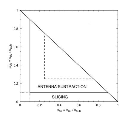
Refer to caption
Figure 9: The phase space for the decay (AB)aub𝐴𝐵𝑎𝑢𝑏(AB)\to aub. The cut min(sau,sub)=δsubscript𝑠𝑎𝑢subscript𝑠𝑢𝑏𝛿\min(s_{au},s_{ub})=\delta with δ=0.1saub𝛿0.1subscript𝑠𝑎𝑢𝑏\delta=0.1~{}s_{aub} is shown as a solid line while min(sau,sub)=Δsubscript𝑠𝑎𝑢subscript𝑠𝑢𝑏Δ\min(s_{au},s_{ub})=\Delta is shown as a dashed line for Δ=0.25saubΔ0.25subscript𝑠𝑎𝑢𝑏\Delta=0.25~{}s_{aub}. The region min(sau,sub)<δsubscript𝑠𝑎𝑢subscript𝑠𝑢𝑏𝛿\min(s_{au},s_{ub})<\delta defines where the slicing approach is utilised, with the soft and collinear regions demarked by dotted lines. Antenna subtraction is applied when δ<min(sau,sub)<Δ𝛿subscript𝑠𝑎𝑢subscript𝑠𝑢𝑏Δ\delta<\min(s_{au},s_{ub})<\Delta.

A.4.1 Quark-Antiquark antenna

Let us first consider a system containing a quark, antiquark and a gluon. This is produced by an antenna comprising of a hard quark and antiquark pair that decays by radiating a gluon. Any function that has the correct soft gluon and collinear quark/gluon singularities in the appropriate limit is satisfactory. Here the hard particles in the antenna are Q𝑄Q and Q¯¯𝑄\overline{Q} which radiate to form q𝑞q, q¯¯𝑞\bar{q} and the gluon g𝑔g. A suitable choice for the antenna function is,

𝒜qgq¯subscript𝒜𝑞𝑔¯𝑞\displaystyle{\cal A}_{qg\bar{q}} =\displaystyle= |𝒮μ(q;g;q¯)Vμ|2|𝒮μ(Q;Q¯)Vμ|2superscriptsubscript𝒮𝜇𝑞𝑔¯𝑞superscript𝑉𝜇2superscriptsubscript𝒮𝜇𝑄¯𝑄superscript𝑉𝜇2\displaystyle\frac{|{\cal S}_{\mu}(q;g;\bar{q})V^{\mu}|^{2}}{|{\cal S}_{\mu}(Q;{\overline{Q}})V^{\mu}|^{2}} (A.29)
=\displaystyle= 2saub(xauxub+xubxau+2xabxaubxauxub).2subscript𝑠𝑎𝑢𝑏subscript𝑥𝑎𝑢subscript𝑥𝑢𝑏subscript𝑥𝑢𝑏subscript𝑥𝑎𝑢2subscript𝑥𝑎𝑏subscript𝑥𝑎𝑢𝑏subscript𝑥𝑎𝑢subscript𝑥𝑢𝑏\displaystyle\frac{2}{s_{aub}}\left(\frac{x_{au}}{x_{ub}}+\frac{x_{ub}}{x_{au}}+\frac{2x_{ab}x_{aub}}{x_{au}x_{ub}}\right).

Because this is proportional to the three parton matrix elements, |𝒮μ(q;g;q¯)Vμ|2superscriptsubscript𝒮𝜇𝑞𝑔¯𝑞superscript𝑉𝜇2|{\cal S}_{\mu}(q;g;\bar{q})V^{\mu}|^{2}, it automatically contains the correct soft and collinear limits. Furthermore, it is smooth over the whole three particle phase space and singularities only appear in the sau0subscript𝑠𝑎𝑢0s_{au}\to 0 and sub0subscript𝑠𝑢𝑏0s_{ub}\to 0 limits.

Explicitly integrating over the antenna phase space for δ<min(sau,sub)<Δ𝛿subscript𝑠𝑎𝑢subscript𝑠𝑢𝑏Δ\delta<\min(s_{au},s_{ub})<\Delta we find,

QQ¯(sQQ¯)subscript𝑄¯𝑄subscript𝑠𝑄¯𝑄\displaystyle{\cal F}_{Q{\overline{Q}}}(s_{Q{\overline{Q}}}) =\displaystyle= (g2N2)𝒜qgq¯dPSsingsuperscript𝑔2𝑁2subscript𝒜𝑞𝑔¯𝑞differential-d𝑃superscript𝑆sing\displaystyle\left(\frac{g^{2}N}{2}\right)\int{\cal A}_{qg\bar{q}}~{}{\rm d}PS^{\rm sing} (A.30)
=\displaystyle= (αsN2π)(ln2(δsQQ¯)+32ln(δsQQ¯))+QQ¯Δ(ΔsQQ¯)+𝒪(δ).subscript𝛼𝑠𝑁2𝜋superscript2𝛿subscript𝑠𝑄¯𝑄32𝛿subscript𝑠𝑄¯𝑄superscriptsubscript𝑄¯𝑄ΔΔsubscript𝑠𝑄¯𝑄𝒪𝛿\displaystyle\left(\frac{\alpha_{s}N}{2\pi}\right)\Biggl{(}\ln^{2}\left(\frac{\delta}{s_{Q{\overline{Q}}}}\right)+\frac{3}{2}\ln\left(\frac{\delta}{s_{Q{\overline{Q}}}}\right)\Biggr{)}+{\cal F}_{Q{\overline{Q}}}^{\Delta}\left(\frac{\Delta}{s_{Q{\overline{Q}}}}\right)+{\cal O}(\delta).

Since we intend to take the δ0𝛿0\delta\to 0 limit, the terms of 𝒪(δ)𝒪𝛿{\cal O}(\delta) may be safely neglected. The δ𝛿\delta independent function QQ¯Δsuperscriptsubscript𝑄¯𝑄Δ{\cal F}_{Q{\overline{Q}}}^{\Delta} is given by,

QQ¯Δ(x)=(αsN2π)(ln2(x)+5x22Li2(x)+(322x+x22)ln(1xx)).superscriptsubscript𝑄¯𝑄Δ𝑥subscript𝛼𝑠𝑁2𝜋superscript2𝑥5𝑥22Lsubscripti2𝑥322𝑥superscript𝑥221𝑥𝑥{\cal F}_{Q{\overline{Q}}}^{\Delta}(x)=\left(\frac{\alpha_{s}N}{2\pi}\right)\Biggl{(}-\ln^{2}\left(x\right)+\frac{5x}{2}-2{\rm Li}_{2}(x)+\left(\frac{3}{2}-2x+\frac{x^{2}}{2}\right)\ln\left(\frac{1-x}{x}\right)\Biggr{)}. (A.31)

A.4.2 Quark-Gluon antenna

For antenna made of a quark Q𝑄Q and gluon G𝐺G, there are two possible ways of radiating. Either a gluon can be radiated so that a quark-gluon-gluon system is formed, or the gluon may split into a antiquark-quark pair. This latter possibility is subleading in the number of colours and the discussion of situations like this is deferred to sec. A.4.4.

For a quark-gluon-gluon system there is a less obvious choice of antenna function, particularly since the singularity that is produced when the gluon splits sits in more than one antenna. If, in the collinear limit, the gluon splits into an unresolved gluon u𝑢u which carries momentum fraction z𝑧z and a hard gluon b𝑏b with momentum fraction 1z1𝑧1-z, the antenna function should naively be proportional to Pgggsubscript𝑃𝑔𝑔𝑔P_{gg\to g} which is singular as z0𝑧0z\to 0 and z1𝑧1z\to 1. This corresponds to singularities as both sub0subscript𝑠𝑢𝑏0s_{ub}\to 0 and sab0subscript𝑠𝑎𝑏0s_{ab}\to 0. However, because the collinear singularity sits in more than one antenna - the two gluons also occur in a second antenna where the role of the two gluons is reversed - we can make use of the N=1𝑁1N=1 supersymmetric identity to rewrite Pgggsubscript𝑃𝑔𝑔𝑔P_{gg\to g} as,

Pggg=Pqgq+PgqqPqq¯g.subscript𝑃𝑔𝑔𝑔subscript𝑃𝑞𝑔𝑞subscript𝑃𝑔𝑞𝑞subscript𝑃𝑞¯𝑞𝑔P_{gg\to g}=P_{qg\to q}+P_{gq\to q}-P_{q\bar{q}\to g}. (A.32)

The soft singularities as z0𝑧0z\to 0 are contained in Pgqqsubscript𝑃𝑔𝑞𝑞P_{gq\to q} while those as z1𝑧1z\to 1 are in Pqgqsubscript𝑃𝑞𝑔𝑞P_{qg\to q}. We therefore divide Pgggsubscript𝑃𝑔𝑔𝑔P_{gg\to g} amongst the two antennae such that Pgqqsubscript𝑃𝑔𝑞𝑞P_{gq\to q} sits in the antenna where gluon u𝑢u is unresolved. The z1𝑧1z\to 1 singularities are placed in the antenna where the role of the two gluons is reversed. The remaining Pqq¯gsubscript𝑃𝑞¯𝑞𝑔P_{q\bar{q}\to g} may be divided between the two antennae according to choice. With a slight modification due to the Pqq¯gsubscript𝑃𝑞¯𝑞𝑔P_{q\bar{q}\to g} term, the antenna function used for the QQ¯𝑄¯𝑄Q{\overline{Q}} antenna has the correct limits, so that,

𝒜qgg=𝒜qgq¯2saub(xau2xubxaub).subscript𝒜𝑞𝑔𝑔subscript𝒜𝑞𝑔¯𝑞2subscript𝑠𝑎𝑢𝑏superscriptsubscript𝑥𝑎𝑢2subscript𝑥𝑢𝑏subscript𝑥𝑎𝑢𝑏{\cal A}_{qgg}={\cal A}_{qg\bar{q}}-\frac{2}{s_{aub}}\left(\frac{x_{au}^{2}}{x_{ub}x_{aub}}\right). (A.33)

This is again smooth over the whole three particle phase space with singularities only appearing in the sau0subscript𝑠𝑎𝑢0s_{au}\to 0 and sub0subscript𝑠𝑢𝑏0s_{ub}\to 0 limits. In particular, as z0𝑧0z\to 0, the collinear limit matches onto the soft limit which would not have been the case if we had divided the soft/collinear singularities equally between the two antenna.

After integrating over the antenna phase space for δ<min(sau,sub)<Δ𝛿subscript𝑠𝑎𝑢subscript𝑠𝑢𝑏Δ\delta<\min(s_{au},s_{ub})<\Delta we find,

QG(sQG)subscript𝑄𝐺subscript𝑠𝑄𝐺\displaystyle{\cal F}_{QG}(s_{QG}) =\displaystyle= (g2N2)𝒜qggdPSsingsuperscript𝑔2𝑁2subscript𝒜𝑞𝑔𝑔differential-d𝑃superscript𝑆sing\displaystyle\left(\frac{g^{2}N}{2}\right)\int{\cal A}_{qgg}~{}{\rm d}PS^{\rm sing} (A.34)
=\displaystyle= (αsN2π)(ln2(δsQG)+106ln(δsQG))+QGΔ(ΔsQG)subscript𝛼𝑠𝑁2𝜋superscript2𝛿subscript𝑠𝑄𝐺106𝛿subscript𝑠𝑄𝐺superscriptsubscript𝑄𝐺ΔΔsubscript𝑠𝑄𝐺\displaystyle\left(\frac{\alpha_{s}N}{2\pi}\right)\Biggl{(}\ln^{2}\left(\frac{\delta}{s_{QG}}\right)+\frac{10}{6}\ln\left(\frac{\delta}{s_{QG}}\right)\Biggr{)}+{\cal F}_{QG}^{\Delta}\left(\frac{\Delta}{s_{QG}}\right)

with the δ𝛿\delta independent function QGΔsuperscriptsubscript𝑄𝐺Δ{\cal F}_{QG}^{\Delta} is given by,

QGΔ(x)superscriptsubscript𝑄𝐺Δ𝑥\displaystyle{\cal F}_{QG}^{\Delta}(x) =\displaystyle= (αsN2π)(ln2(x)+19x6x26+x392Li2(x)\displaystyle\left(\frac{\alpha_{s}N}{2\pi}\right)\Biggl{(}-\ln^{2}\left(x\right)+\frac{19x}{6}-\frac{x^{2}}{6}+\frac{x^{3}}{9}-2{\rm Li}_{2}(x) (A.35)
+(1062x+x22x36)ln(1xx)).\displaystyle~{}~{}~{}~{}~{}~{}~{}~{}~{}~{}~{}+\left(\frac{10}{6}-2x+\frac{x^{2}}{2}-\frac{x^{3}}{6}\right)\ln\left(\frac{1-x}{x}\right)\Biggr{)}.

Antennae containing a gluon and an antiquark are described by,

𝒜ggq¯=𝒜qgg(ab),{\cal A}_{gg\bar{q}}={\cal A}_{qgg}(a\leftrightarrow b), (A.36)

and,

GQ¯(sGQ¯)=QG(sGQ¯).subscript𝐺¯𝑄subscript𝑠𝐺¯𝑄subscript𝑄𝐺subscript𝑠𝐺¯𝑄{\cal F}_{G{\overline{Q}}}(s_{G{\overline{Q}}})={\cal F}_{QG}(s_{G{\overline{Q}}}). (A.37)

A.4.3 Gluon-Gluon antenna

For antenna comprising only gluons, we repeat this SUSY inspired trick for each of the resolved gluons so that,

𝒜ggg=𝒜qgq¯2saub(xau2xubxaub+xub2xauxaub).subscript𝒜𝑔𝑔𝑔subscript𝒜𝑞𝑔¯𝑞2subscript𝑠𝑎𝑢𝑏superscriptsubscript𝑥𝑎𝑢2subscript𝑥𝑢𝑏subscript𝑥𝑎𝑢𝑏superscriptsubscript𝑥𝑢𝑏2subscript𝑥𝑎𝑢subscript𝑥𝑎𝑢𝑏{\cal A}_{ggg}={\cal A}_{qg\bar{q}}-\frac{2}{s_{aub}}\left(\frac{x_{au}^{2}}{x_{ub}x_{aub}}+\frac{x_{ub}^{2}}{x_{au}x_{aub}}\right). (A.38)

Note that Kosower [42] has proposed an antenna factorisation for gluonic processes,

𝒜gggKosower=4saub((xaub(xaubxab)+xab2)2xauxubxabxsub),superscriptsubscript𝒜𝑔𝑔𝑔Kosower4subscript𝑠𝑎𝑢𝑏superscriptsubscript𝑥𝑎𝑢𝑏subscript𝑥𝑎𝑢𝑏subscript𝑥𝑎𝑏superscriptsubscript𝑥𝑎𝑏22subscript𝑥𝑎𝑢subscript𝑥𝑢𝑏subscript𝑥𝑎𝑏subscript𝑥𝑠𝑢𝑏{\cal A}_{ggg}^{\rm Kosower}=\frac{4}{s_{aub}}\left(\frac{(x_{aub}(x_{aub}-x_{ab})+x_{ab}^{2})^{2}}{x_{au}x_{ub}x_{ab}x_{sub}}\right), (A.39)

which, in the u/b𝑢𝑏u/b collinear limit regenerates the full Pgggsubscript𝑃𝑔𝑔𝑔P_{gg\to g} splitting function, as well as the soft limits.

Integration of the antenna function 𝒜gggsubscript𝒜𝑔𝑔𝑔{\cal A}_{ggg} over the whole of the subtraction region yields,

GG(sGG)subscript𝐺𝐺subscript𝑠𝐺𝐺\displaystyle{\cal F}_{GG}(s_{GG}) =\displaystyle= (g2N2)𝒜gggdPSsingsuperscript𝑔2𝑁2subscript𝒜𝑔𝑔𝑔differential-d𝑃superscript𝑆sing\displaystyle\left(\frac{g^{2}N}{2}\right)\int{\cal A}_{ggg}~{}{\rm d}PS^{\rm sing} (A.40)
=\displaystyle= (αsN2π)(ln2(δsGG)+116ln(δsGG))+GGΔ(ΔsGG)subscript𝛼𝑠𝑁2𝜋superscript2𝛿subscript𝑠𝐺𝐺116𝛿subscript𝑠𝐺𝐺superscriptsubscript𝐺𝐺ΔΔsubscript𝑠𝐺𝐺\displaystyle\left(\frac{\alpha_{s}N}{2\pi}\right)\Biggl{(}\ln^{2}\left(\frac{\delta}{s_{GG}}\right)+\frac{11}{6}\ln\left(\frac{\delta}{s_{GG}}\right)\Biggr{)}+{\cal F}_{GG}^{\Delta}\left(\frac{\Delta}{s_{GG}}\right)

with the δ𝛿\delta independent function GGΔsuperscriptsubscript𝐺𝐺Δ{\cal F}_{GG}^{\Delta} is given by,

GGΔ(x)superscriptsubscript𝐺𝐺Δ𝑥\displaystyle{\cal F}_{GG}^{\Delta}(x) =\displaystyle= (αsN2π)(ln2(x)+23x62x26+2x392Li2(x)\displaystyle\left(\frac{\alpha_{s}N}{2\pi}\right)\Biggl{(}-\ln^{2}\left(x\right)+\frac{23x}{6}-\frac{2x^{2}}{6}+\frac{2x^{3}}{9}-2{\rm Li}_{2}(x) (A.41)
+(1162x+x22x33)ln(1xx)).\displaystyle~{}~{}~{}~{}~{}~{}~{}~{}~{}~{}~{}+\left(\frac{11}{6}-2x+\frac{x^{2}}{2}-\frac{x^{3}}{3}\right)\ln\left(\frac{1-x}{x}\right)\Biggr{)}.

A.4.4 Antenna where a quark-antiquark pair merge

There are also configurations when two (or more) colour lines are present, one ending in an antiquark the other starting with a quark of the same flavour. Here the matrix elements have the form,

|𝒮μ(,a,q¯|q,b,)Vμ|2.\Big{|}{\cal S}_{\mu}(\ldots,a,\bar{q}|q,b,\ldots)V^{\mu}\Big{|}^{2}. (A.42)

In the collinear limit, the quark-antiquark pinch the two colour lines together to form a single colour line,

|𝒮μ(,a,q¯|q,b,)Vμ|2Pq¯qg(z,sq¯q)|𝒮μ(,a,G,b,)Vμ|2,\Big{|}{\cal S}_{\mu}(\ldots,a,\bar{q}|q,b,\ldots)V^{\mu}\Big{|}^{2}\to P_{\bar{q}q\to g}(z,s_{\bar{q}q})\Big{|}{\cal S}_{\mu}(\ldots,a,G,b,\ldots)V^{\mu}\Big{|}^{2}, (A.43)

with Pq¯qG(z,s)subscript𝑃¯𝑞𝑞𝐺𝑧𝑠P_{\bar{q}q\to G}(z,s) given by eqs. (A.12) and (A.15). There is no soft singularity, nor is there any dependence on the type of adjacent parton, a𝑎a or b𝑏b. Clearly, the quark-antiquark pair can sit in two antennae, (a,q¯,q)𝑎¯𝑞𝑞(a,\bar{q},q) and (q¯,q,b)¯𝑞𝑞𝑏(\bar{q},q,b) and we have some freedom of how to assign the singularities to the antennae. There are two obvious choices. Either we divide the singular contribution equally over the two antennae, or, we place the z2superscript𝑧2z^{2} part of Pq¯qg(z)subscript𝑃¯𝑞𝑞𝑔𝑧P_{\bar{q}q\to g}(z) in one antenna and the (1z)2superscript1𝑧2(1-z)^{2} part in the other (as we did with the three gluon antenna before). While there appears to be no preference, we follow this latter route so that the antenna function vanishes as the unresolved particle becomes soft,

𝒜aq¯q=2saq¯q(xaq¯2xq¯qxaq¯q),subscript𝒜𝑎¯𝑞𝑞2subscript𝑠𝑎¯𝑞𝑞superscriptsubscript𝑥𝑎¯𝑞2subscript𝑥¯𝑞𝑞subscript𝑥𝑎¯𝑞𝑞{\cal A}_{a\bar{q}q}=\frac{2}{s_{a\bar{q}q}}\left(\frac{x_{a\bar{q}}^{2}}{x_{\bar{q}q}x_{a\bar{q}q}}\right), (A.44)

and,

𝒜q¯qb=𝒜aq¯q(xaq¯xqb,xaq¯qxq¯qb).{\cal A}_{\bar{q}qb}={\cal A}_{a\bar{q}q}(x_{a\bar{q}}\to x_{qb},x_{a\bar{q}q}\leftrightarrow x_{\bar{q}qb}). (A.45)

Following this procedure and integrating over the whole of the subtraction region yields,

aGNF(saG)subscriptsuperscriptsubscript𝑁𝐹𝑎𝐺subscript𝑠𝑎𝐺\displaystyle{\cal F}^{N_{F}}_{aG}(s_{aG}) =\displaystyle= (g2NF2)𝒜aq¯qdPSsingsuperscript𝑔2subscript𝑁𝐹2subscript𝒜𝑎¯𝑞𝑞differential-d𝑃superscript𝑆sing\displaystyle\left(\frac{g^{2}N_{F}}{2}\right)\int{\cal A}_{a\bar{q}q}~{}{\rm d}PS^{\rm sing} (A.46)
=\displaystyle= (αsNF2π)(16ln(δsaG))+aGNFΔ(ΔsaG),subscript𝛼𝑠subscript𝑁𝐹2𝜋16𝛿subscript𝑠𝑎𝐺superscriptsubscript𝑎𝐺subscript𝑁𝐹ΔΔsubscript𝑠𝑎𝐺\displaystyle\left(\frac{\alpha_{s}N_{F}}{2\pi}\right)\Biggl{(}-\frac{1}{6}\ln\left(\frac{\delta}{s_{aG}}\right)\Biggr{)}+{\cal F}_{aG}^{N_{F}\Delta}\left(\frac{\Delta}{s_{aG}}\right),

and,

GbNF(sGb)=aGNF(sGb).subscriptsuperscriptsubscript𝑁𝐹𝐺𝑏subscript𝑠𝐺𝑏subscriptsuperscriptsubscript𝑁𝐹𝑎𝐺subscript𝑠𝐺𝑏{\cal F}^{N_{F}}_{Gb}(s_{Gb})={\cal F}^{N_{F}}_{aG}(s_{Gb}). (A.47)

The factor of NFsubscript𝑁𝐹N_{F} arises because each of the NFsubscript𝑁𝐹N_{F} quark flavours may contribute. The δ𝛿\delta independent function is,

aGNFΔ(x)superscriptsubscript𝑎𝐺subscript𝑁𝐹Δ𝑥\displaystyle{\cal F}_{aG}^{N_{F}\Delta}(x) =\displaystyle= GbNFΔ(x)superscriptsubscript𝐺𝑏subscript𝑁𝐹Δ𝑥\displaystyle{\cal F}_{Gb}^{N_{F}\Delta}(x) (A.48)
=\displaystyle= (αsNF2π)(2x3+x26x39(16x36)ln(1xx)).subscript𝛼𝑠subscript𝑁𝐹2𝜋2𝑥3superscript𝑥26superscript𝑥3916superscript𝑥361𝑥𝑥\displaystyle\left(\frac{\alpha_{s}N_{F}}{2\pi}\right)\Biggl{(}-\frac{2x}{3}+\frac{x^{2}}{6}-\frac{x^{3}}{9}-\left(\frac{1}{6}-\frac{x^{3}}{6}\right)\ln\left(\frac{1-x}{x}\right)\Biggr{)}.

A.5 Leading colour contribution to e+e4superscript𝑒superscript𝑒4e^{+}e^{-}\to 4 jets.

As a pedagogical example, we consider the leading colour contribution relevant for e+e4superscript𝑒superscript𝑒4e^{+}e^{-}\to 4 jets. The sub-leading pieces are similarly calculated but the resulting expressions are somewhat lengthy due to the many antennae that are involved [40]. At leading order in the number of colours, only the two quark and n𝑛n gluon process contributes666The four quark process gives a contribution that is suppressed by a factor of NF/Nsubscript𝑁𝐹𝑁N_{F}/N relative to the leading colour contribution. Numerically this is an important contribution and, together with the other subleading terms, is included in the numerical results presented earlier., so, at lowest order, the cross section is given by,

dσ4LOσ0dsuperscriptsubscript𝜎4LOsubscript𝜎0\displaystyle\frac{{\rm d}\sigma_{4}^{\rm LO}}{\sigma_{0}} =\displaystyle= (2π)5s(N21N2)(αsN2π)2superscript2𝜋5𝑠superscript𝑁21superscript𝑁2superscriptsubscript𝛼𝑠𝑁2𝜋2\displaystyle\frac{(2\pi)^{5}}{s}\left(\frac{N^{2}-1}{N^{2}}\right)\left(\frac{\alpha_{s}N}{2\pi}\right)^{2} (A.49)
×\displaystyle\times P(G1,G2)|𝒮μ(Q1;G1,G2;Q¯2)Vμ|2𝒥(4)dPS(Q2;Q1G1,G2,Q¯2)2,subscript𝑃subscript𝐺1subscript𝐺2superscriptsubscript𝒮𝜇subscript𝑄1subscript𝐺1subscript𝐺2subscript¯𝑄2superscript𝑉𝜇2subscript𝒥4d𝑃𝑆superscript𝑄2subscript𝑄1subscript𝐺1subscript𝐺2subscript¯𝑄2subscript2\displaystyle\sum_{P(G_{1},G_{2})}\Big{|}{\cal S}_{\mu}(Q_{1};G_{1},G_{2};{\overline{Q}}_{2})V^{\mu}\Big{|}^{2}~{}{\cal J}_{(4)}~{}{\rm d}PS(Q^{2};Q_{1}G_{1},G_{2},{\overline{Q}}_{2}){\cal I}_{2},

where 2subscript2{\cal I}_{2} is the identical particle factor for the two gluon final state. In practice, the 2!22! permutations precisely cancels the identical particle factor of 1/2!121/2!, and it is more convenient to keep one particular ordering so that,

dσ4LOσ0=(2π)5s(N21N2)(αsN2π)2|𝒮μ(Q1;G1,G2;Q¯2)Vμ|2𝒥(4)dPS(Q2;Q1G1,G2,Q¯2).dsuperscriptsubscript𝜎4LOsubscript𝜎0superscript2𝜋5𝑠superscript𝑁21superscript𝑁2superscriptsubscript𝛼𝑠𝑁2𝜋2superscriptsubscript𝒮𝜇subscript𝑄1subscript𝐺1subscript𝐺2subscript¯𝑄2superscript𝑉𝜇2subscript𝒥4d𝑃𝑆superscript𝑄2subscript𝑄1subscript𝐺1subscript𝐺2subscript¯𝑄2\frac{{\rm d}\sigma_{4}^{\rm LO}}{\sigma_{0}}=\frac{(2\pi)^{5}}{s}\left(\frac{N^{2}-1}{N^{2}}\right)\left(\frac{\alpha_{s}N}{2\pi}\right)^{2}\Big{|}{\cal S}_{\mu}(Q_{1};G_{1},G_{2};{\overline{Q}}_{2})V^{\mu}\Big{|}^{2}~{}{\cal J}_{(4)}~{}{\rm d}PS(Q^{2};Q_{1}G_{1},G_{2},{\overline{Q}}_{2}). (A.50)

Similarly, the leading colour contribution from the five parton bremstrahlung process is,

dσ5σ0dsubscript𝜎5subscript𝜎0\displaystyle\frac{{\rm d}\sigma_{5}}{\sigma_{0}} =\displaystyle= (2π)7s(N21N2)(αsN2π)3superscript2𝜋7𝑠superscript𝑁21superscript𝑁2superscriptsubscript𝛼𝑠𝑁2𝜋3\displaystyle\frac{(2\pi)^{7}}{s}\left(\frac{N^{2}-1}{N^{2}}\right)\left(\frac{\alpha_{s}N}{2\pi}\right)^{3}
×\displaystyle\times P(g1,g2,g3)|𝒮μ(q1;g1,g2,g3;q¯2)Vμ|2𝒥(5)dPS(Q2;q1,g1,g2,g3,q¯2)3,subscript𝑃subscript𝑔1subscript𝑔2subscript𝑔3superscriptsubscript𝒮𝜇subscript𝑞1subscript𝑔1subscript𝑔2subscript𝑔3subscript¯𝑞2superscript𝑉𝜇2subscript𝒥5d𝑃𝑆superscript𝑄2subscript𝑞1subscript𝑔1subscript𝑔2subscript𝑔3subscript¯𝑞2subscript3\displaystyle\sum_{P(g_{1},g_{2},g_{3})}\Big{|}{\cal S}_{\mu}(q_{1};g_{1},g_{2},g_{3};\bar{q}_{2})V^{\mu}\Big{|}^{2}~{}{\cal J}_{(5)}~{}{\rm d}PS(Q^{2};q_{1},g_{1},g_{2},g_{3},\bar{q}_{2}){\cal I}_{3},
=\displaystyle= (2π)7s(N21N2)(αsN2π)3|𝒮μ(q1;g1,g2,g3;q¯2)Vμ|2𝒥(5)dPS(Q2;q1,g1,g2,g3,q¯2).superscript2𝜋7𝑠superscript𝑁21superscript𝑁2superscriptsubscript𝛼𝑠𝑁2𝜋3superscriptsubscript𝒮𝜇subscript𝑞1subscript𝑔1subscript𝑔2subscript𝑔3subscript¯𝑞2superscript𝑉𝜇2subscript𝒥5d𝑃𝑆superscript𝑄2subscript𝑞1subscript𝑔1subscript𝑔2subscript𝑔3subscript¯𝑞2\displaystyle\frac{(2\pi)^{7}}{s}\left(\frac{N^{2}-1}{N^{2}}\right)\left(\frac{\alpha_{s}N}{2\pi}\right)^{3}\Big{|}{\cal S}_{\mu}(q_{1};g_{1},g_{2},g_{3};\bar{q}_{2})V^{\mu}\Big{|}^{2}~{}{\cal J}_{(5)}~{}{\rm d}PS(Q^{2};q_{1},g_{1},g_{2},g_{3},\bar{q}_{2}).

Note that 𝒥5subscript𝒥5{\cal J}_{5} projects the five parton momenta onto the four jet like observable. Once again, we can cancel the identical particle factor 3=1/3!subscript313{\cal I}_{3}=1/3! against the 3!33! permutations of the gluons, and retain the single permutation indicated. For this colour ordering, three antennae will contribute, (q1,g1,g2)subscript𝑞1subscript𝑔1subscript𝑔2(q_{1},g_{1},g_{2}), (g1,g2,g3)subscript𝑔1subscript𝑔2subscript𝑔3(g_{1},g_{2},g_{3}) and (g2,g3,q¯2)subscript𝑔2subscript𝑔3subscript¯𝑞2(g_{2},g_{3},\bar{q}_{2}) where in each case the parton in the middle is unresolved. In the first antenna, {pq1,pg1,pg2}{pQ1,pG1}subscript𝑝subscript𝑞1subscript𝑝subscript𝑔1subscript𝑝subscript𝑔2subscript𝑝subscript𝑄1subscript𝑝subscript𝐺1\{p_{q_{1}},p_{g_{1}},p_{g_{2}}\}\to\{p_{Q_{1}},p_{G_{1}}\} according to eq. (LABEL:eq:transform), the slicing cuts are min(sq1g1,sg1g2)<δsubscript𝑠subscript𝑞1subscript𝑔1subscript𝑠subscript𝑔1subscript𝑔2𝛿\min(s_{q_{1}g_{1}},s_{g_{1}g_{2}})<\delta and the subtraction occurs over the range δ<min(sq1g1,sg1g2)<Δ𝛿subscript𝑠subscript𝑞1subscript𝑔1subscript𝑠subscript𝑔1subscript𝑔2Δ\delta<\min(s_{q_{1}g_{1}},s_{g_{1}g_{2}})<\Delta. Similar transformations and cuts act over the other two antenna.

A.5.1 Slicing contribution

For the five parton matrix elements of eq. (LABEL:eq:sig5), the sum of infrared singularities from the three antennae in the slicing approach gives a contribution to the four particle final state which can be read directly from eq. (3.79) of ref. [18],

dσ4slice=R(Q1;G1,G2;Q¯2)dσ4LO.dsuperscriptsubscript𝜎4slice𝑅subscript𝑄1subscript𝐺1subscript𝐺2subscript¯𝑄2dsuperscriptsubscript𝜎4LO{\rm d}\sigma_{4}^{\rm slice}=R(Q_{1};G_{1},G_{2};{\overline{Q}}_{2}){\rm d}\sigma_{4}^{\rm LO}. (A.52)

Retaining only the leading colour contribution (i.e. dropping the contributions from the four quark process proportional to the number of quark flavours),

R(Q1;G1,G2;Q¯2)𝑅subscript𝑄1subscript𝐺1subscript𝐺2subscript¯𝑄2\displaystyle R(Q_{1};G_{1},G_{2};{\overline{Q}}_{2}) =\displaystyle= (αsN2π)1Γ(1ϵ)[ij{1ϵ2(4πμ2sij)ϵlog2(sijδ)}\displaystyle\left(\frac{\alpha_{s}N}{2\pi}\right)\frac{1}{\Gamma(1-\epsilon)}~{}\Biggl{[}\sum_{ij}\left\{\frac{1}{\epsilon^{2}}\left(\frac{4\pi\mu^{2}}{s_{ij}}\right)^{\epsilon}-\log^{2}\left(\frac{s_{ij}}{\delta}\right)\right\}
+32ϵ(4πμ2δ)ϵ+19718π2]\displaystyle+\frac{3}{2\epsilon}\left(\frac{4\pi\mu^{2}}{\delta}\right)^{\epsilon}+\frac{197}{18}-\pi^{2}\Biggr{]}
+\displaystyle+ (αs2π)2b0ϵ1Γ(1ϵ)(4πμ2δ)ϵ+𝒪(ϵ)+𝒪(δ),subscript𝛼𝑠2𝜋2subscript𝑏0italic-ϵ1Γ1italic-ϵsuperscript4𝜋superscript𝜇2𝛿italic-ϵ𝒪italic-ϵ𝒪𝛿\displaystyle\left(\frac{\alpha_{s}}{2\pi}\right)\frac{2b_{0}}{\epsilon}\frac{1}{\Gamma(1-\epsilon)}\left(\frac{4\pi\mu^{2}}{\delta}\right)^{\epsilon}+{\cal O}(\epsilon)+{\cal O}(\delta),

with (at leading order in the number of colours) b0=11N/6subscript𝑏011𝑁6b_{0}=11N/6 and where the sum runs over the pairs of adjacent (colour connected) hard partons, ij=Q1G1𝑖𝑗subscript𝑄1subscript𝐺1ij=Q_{1}G_{1}, G1G2subscript𝐺1subscript𝐺2G_{1}G_{2} and G2Q¯2subscript𝐺2subscript¯𝑄2G_{2}{\overline{Q}}_{2}.

A.5.2 Subtraction term

Since there are three antennae, we subtract three antennae factors, such that the total subtraction term is,

dσ5subσ0dsuperscriptsubscript𝜎5subsubscript𝜎0\displaystyle\frac{{\rm d}\sigma_{5}^{\rm sub}}{\sigma_{0}} =\displaystyle= (2π)7s(N21N2)(αsN2π)3dPS(Q2;q1,g1,g2,g3,q¯2)superscript2𝜋7𝑠superscript𝑁21superscript𝑁2superscriptsubscript𝛼𝑠𝑁2𝜋3d𝑃𝑆superscript𝑄2subscript𝑞1subscript𝑔1subscript𝑔2subscript𝑔3subscript¯𝑞2\displaystyle\frac{(2\pi)^{7}}{s}\left(\frac{N^{2}-1}{N^{2}}\right)\left(\frac{\alpha_{s}N}{2\pi}\right)^{3}~{}{\rm d}PS(Q^{2};q_{1},g_{1},g_{2},g_{3},\bar{q}_{2}) (A.53)
×\displaystyle\times (𝒜q1g1g2|𝒮μ(Q1;G1,g3;q¯2)Vμ|2𝒥(4)\displaystyle\Biggl{(}~{}{\cal A}_{q_{1}g_{1}g_{2}}\Big{|}{\cal S}_{\mu}(Q_{1};G_{1},g_{3};\bar{q}_{2})V^{\mu}\Big{|}^{2}~{}{\cal J}_{(4)}
+𝒜g1g2g3|𝒮μ(q1;G1,G2;q¯2)Vμ|2𝒥(4)subscript𝒜subscript𝑔1subscript𝑔2subscript𝑔3superscriptsubscript𝒮𝜇subscript𝑞1subscript𝐺1subscript𝐺2subscript¯𝑞2superscript𝑉𝜇2subscript𝒥4\displaystyle+~{}{\cal A}_{g_{1}g_{2}g_{3}}\Big{|}{\cal S}_{\mu}(q_{1};G_{1},G_{2};\bar{q}_{2})V^{\mu}\Big{|}^{2}~{}{\cal J}_{(4)}
+𝒜g2g2q¯2|𝒮μ(q1;g1,G2;Q¯2)Vμ|2𝒥(4)).\displaystyle+~{}{\cal A}_{g_{2}g_{2}\bar{q}_{2}}\Big{|}{\cal S}_{\mu}(q_{1};g_{1},G_{2};{\overline{Q}}_{2})V^{\mu}\Big{|}^{2}~{}{\cal J}_{(4)}~{}\Biggr{)}.

Here, we have used the mappings {pq1,pg1,pg2}{pQ1,pG1}subscript𝑝subscript𝑞1subscript𝑝subscript𝑔1subscript𝑝subscript𝑔2subscript𝑝subscript𝑄1subscript𝑝subscript𝐺1\{p_{q_{1}},p_{g_{1}},p_{g_{2}}\}\to\{p_{Q_{1}},p_{G_{1}}\} according to eq. (LABEL:eq:transform) for the first antenna. We recall that the subtraction occurs over the range δ<min(sq1g1,sg1g2)<Δ𝛿subscript𝑠subscript𝑞1subscript𝑔1subscript𝑠subscript𝑔1subscript𝑔2Δ\delta<\min(s_{q_{1}g_{1}},s_{g_{1}g_{2}})<\Delta and that the observable function 𝒥4subscript𝒥4{\cal J}_{4} is applied to the momenta for Q1subscript𝑄1Q_{1}, G1subscript𝐺1G_{1}, g3subscript𝑔3g_{3} and q¯2subscript¯𝑞2\bar{q}_{2}. Similar procedures are applied to the other antennae.

However, we must add these terms back to the four parton contribution. Here it is simplest to re-identify each of the four particle momenta with the momenta relevant for tree level. In other words, for the first antenna, {pq1,pg1,pg2}{pQ1,pG1}subscript𝑝subscript𝑞1subscript𝑝subscript𝑔1subscript𝑝subscript𝑔2subscript𝑝subscript𝑄1subscript𝑝subscript𝐺1\{p_{q_{1}},p_{g_{1}},p_{g_{2}}\}\to\{p_{Q_{1}},p_{G_{1}}\} as before and pg3pG2subscript𝑝subscript𝑔3subscript𝑝subscript𝐺2p_{g_{3}}\to p_{G_{2}}, pq¯2pQ¯2subscript𝑝subscript¯𝑞2subscript𝑝subscript¯𝑄2p_{\bar{q}_{2}}\to p_{{\overline{Q}}_{2}}. This is safe to do since we integrate over the whole four particle phase space. Altogether, we have,

dσ4sub=(Q1G1+G1G2+G2Q¯2)dσ4LO.dsuperscriptsubscript𝜎4subsubscriptsubscript𝑄1subscript𝐺1subscriptsubscript𝐺1subscript𝐺2subscriptsubscript𝐺2subscript¯𝑄2dsuperscriptsubscript𝜎4LO{\rm d}\sigma_{4}^{\rm sub}=\left({\cal F}_{Q_{1}G_{1}}+{\cal F}_{G_{1}G_{2}}+{\cal F}_{G_{2}{\overline{Q}}_{2}}\right){\rm d}\sigma_{4}^{\rm LO}. (A.54)

A.5.3 Virtual contribution

From ref. [7], the matrix elements for the leading colour one-loop contribution to the qq¯gg𝑞¯𝑞𝑔𝑔q\bar{q}gg final state for this colour ordering can be written in terms of a pole structure in ϵitalic-ϵ\epsilon multiplying the lowest order matrix elements and a function ^Asubscript^𝐴\hat{\cal L}_{A} that is finite as ϵ0italic-ϵ0\epsilon\to 0,

A(G1,G2)=V(Q1;G1,G2;Q¯2)|𝒮μ(Q1;G1,G2;Q¯2)Vμ|2+^A(G1,G2).subscript𝐴subscript𝐺1subscript𝐺2𝑉subscript𝑄1subscript𝐺1subscript𝐺2subscript¯𝑄2superscriptsubscript𝒮𝜇subscript𝑄1subscript𝐺1subscript𝐺2subscript¯𝑄2superscript𝑉𝜇2subscript^𝐴subscript𝐺1subscript𝐺2{\cal L}_{A}(G_{1},G_{2})=V(Q_{1};G_{1},G_{2};{\overline{Q}}_{2})\Big{|}{\cal S}_{\mu}(Q_{1};G_{1},G_{2};{\overline{Q}}_{2})V^{\mu}\Big{|}^{2}+\hat{\cal L}_{A}(G_{1},G_{2}). (A.55)

The divergent factor V𝑉V is given by,

V(Q1;G1,G2;Q¯2)=(αsN2π)(𝒫(sQ1G1)ϵ2𝒫(sG2Q¯2)ϵ2𝒫(sG1G2)ϵ232𝒫(Q2)ϵ)𝑉subscript𝑄1subscript𝐺1subscript𝐺2subscript¯𝑄2subscript𝛼𝑠𝑁2𝜋𝒫subscript𝑠subscript𝑄1subscript𝐺1superscriptitalic-ϵ2𝒫subscript𝑠subscript𝐺2subscript¯𝑄2superscriptitalic-ϵ2𝒫subscript𝑠subscript𝐺1subscript𝐺2superscriptitalic-ϵ232𝒫superscript𝑄2italic-ϵV(Q_{1};G_{1},G_{2};{\overline{Q}}_{2})=\left(\frac{\alpha_{s}N}{2\pi}\right)\left(-\frac{{\cal P}(s_{Q_{1}G_{1}})}{\epsilon^{2}}-\frac{{\cal P}(s_{G_{2}{\overline{Q}}_{2}})}{\epsilon^{2}}-\frac{{\cal P}(s_{G_{1}G_{2}})}{\epsilon^{2}}-\frac{3}{2}\frac{{\cal P}(Q^{2})}{\epsilon}\right) (A.56)

where we have introduced the notation,

𝒫(s)=(4πμ2s)ϵΓ2(1ϵ)Γ(1+ϵ)Γ(12ϵ).𝒫𝑠superscript4𝜋superscript𝜇2𝑠italic-ϵsuperscriptΓ21italic-ϵΓ1italic-ϵΓ12italic-ϵ{\cal P}(s)=\left(\frac{4\pi\mu^{2}}{-s}\right)^{\epsilon}\frac{\Gamma^{2}(1-\epsilon)\Gamma(1+\epsilon)}{\Gamma(1-2\epsilon)}. (A.57)

In terms of cross sections, we have,

dσ4V=V(Q1;G1,G2;Q¯2)dσ4LO+dσ4V,finite,dsuperscriptsubscript𝜎4V𝑉subscript𝑄1subscript𝐺1subscript𝐺2subscript¯𝑄2dsuperscriptsubscript𝜎4LOdsuperscriptsubscript𝜎4Vfinite{\rm d}\sigma_{4}^{\rm V}=V(Q_{1};G_{1},G_{2};{\overline{Q}}_{2}){\rm d}\sigma_{4}^{\rm LO}+{\rm d}\sigma_{4}^{\rm V,finite}, (A.58)

with,

dσ4V,finiteσ0=(2π)5s(N21N2)(αsN2π)3^A(G1,G2)𝒥(4)dPS(Q2;pQ1,pG1,pG2,pQ¯2)dsuperscriptsubscript𝜎4Vfinitesubscript𝜎0superscript2𝜋5𝑠superscript𝑁21superscript𝑁2superscriptsubscript𝛼𝑠𝑁2𝜋3subscript^𝐴subscript𝐺1subscript𝐺2subscript𝒥4d𝑃𝑆superscript𝑄2subscript𝑝subscript𝑄1subscript𝑝subscript𝐺1subscript𝑝subscript𝐺2subscript𝑝subscript¯𝑄2\frac{{\rm d}\sigma_{4}^{\rm V,finite}}{\sigma_{0}}=\frac{(2\pi)^{5}}{s}\left(\frac{N^{2}-1}{N^{2}}\right)\left(\frac{\alpha_{s}N}{2\pi}\right)^{3}\hat{\cal L}_{A}(G_{1},G_{2})~{}{\cal J}_{(4)}~{}{\rm d}PS(Q^{2};p_{Q_{1}},p_{G_{1}},p_{G_{2}},p_{{\overline{Q}}_{2}}) (A.59)

Here ^Asubscript^𝐴\hat{\cal L}_{A} is a finite function given in terms of that logarithms and dilogarithms that arise in evaluating the one-loop contributions.777Note that ^Asubscript^𝐴\hat{\cal L}_{A} defined here is a factor of 8 smaller than that in [7]. We have ensured that the kinematic singularity structure of ^Asubscript^𝐴\hat{\cal L}_{A} matches that of the tree-level |𝒮μ(Q1;G1,G2;Q¯2)Vμ|2superscriptsubscript𝒮𝜇subscript𝑄1subscript𝐺1subscript𝐺2subscript¯𝑄2superscript𝑉𝜇2\Big{|}{\cal S}_{\mu}(Q_{1};G_{1},G_{2};{\overline{Q}}_{2})V^{\mu}\Big{|}^{2}. It can be written symbolically as,

^A=iPi(s)Li,subscript^𝐴subscript𝑖subscript𝑃𝑖𝑠subscriptL𝑖\hat{\cal L}_{A}=\sum_{i}P_{i}(s){\rm L}_{i}, (A.60)

where the coefficients Pi(s)subscript𝑃𝑖𝑠P_{i}(s) are rational polynomials of invariants. The finite functions LisubscriptL𝑖{\rm L}_{i} are the linear combinations of scalar integrals defined in [7] which are well-behaved in all kinematic limits, so that ^Asubscript^𝐴\hat{\cal L}_{A} is numerically stable. Unfortunately, the analytic expression for ^Asubscript^𝐴\hat{\cal L}_{A} is rather lengthy so we do not reproduce it here.

A.5.4 Next-to-leading order cross section

Assembling the various pieces, and applying coupling constant renormalisation,

(αs2π)(αs(μ)2π)(1b0(αs(μ)2π)(4π)ϵϵΓ(1ϵ),\left(\frac{\alpha_{s}}{2\pi}\right)\to\left(\frac{\alpha_{s}(\mu)}{2\pi}\right)\left(1-b_{0}\left(\frac{\alpha_{s}(\mu)}{2\pi}\right)\frac{(4\pi)^{\epsilon}}{\epsilon\Gamma(1-\epsilon}\right), (A.61)

the NLO four parton contribution is,

dσ4NLOdsuperscriptsubscript𝜎4NLO\displaystyle{\rm d}\sigma_{4}^{\rm NLO} =\displaystyle= dσ4V+dσ4sub+dσ4slicedsuperscriptsubscript𝜎4Vdsuperscriptsubscript𝜎4subdsuperscriptsubscript𝜎4slice\displaystyle{\rm d}\sigma_{4}^{\rm V}+{\rm d}\sigma_{4}^{\rm sub}+{\rm d}\sigma_{4}^{\rm slice} (A.62)
=\displaystyle= K(Q1;G1,G2;Q¯2)dσ4LO+dσ4V,finite,𝐾subscript𝑄1subscript𝐺1subscript𝐺2subscript¯𝑄2dsuperscriptsubscript𝜎4LOdsuperscriptsubscript𝜎4Vfinite\displaystyle K(Q_{1};G_{1},G_{2};{\overline{Q}}_{2}){\rm d}\sigma_{4}^{\rm LO}+{\rm d}\sigma_{4}^{\rm V,finite},

where dσ4LOdsuperscriptsubscript𝜎4LO{\rm d}\sigma_{4}^{\rm LO} and dσ4V,finitedsuperscriptsubscript𝜎4Vfinite{\rm d}\sigma_{4}^{\rm V,finite} are given by eqs. (A.49) and (A.59) respectively with the replacement αsαs(μ)subscript𝛼𝑠subscript𝛼𝑠𝜇\alpha_{s}\to\alpha_{s}(\mu). The factor K𝐾K is the sum of the divergent one loop factor (eq. (A.56)), the slicing factor (eq. (A.5.1)) and the subtraction term (eq. (A.54)),

K(Q1;G1,G2;Q¯2)𝐾subscript𝑄1subscript𝐺1subscript𝐺2subscript¯𝑄2\displaystyle K(Q_{1};G_{1},G_{2};{\overline{Q}}_{2}) =\displaystyle= V(Q1;G1,G2;Q¯2)+R(Q1;G1,G2;Q¯2)𝑉subscript𝑄1subscript𝐺1subscript𝐺2subscript¯𝑄2𝑅subscript𝑄1subscript𝐺1subscript𝐺2subscript¯𝑄2\displaystyle V(Q_{1};G_{1},G_{2};{\overline{Q}}_{2})+R(Q_{1};G_{1},G_{2};{\overline{Q}}_{2}) (A.63)
+Q1G1(sQ1G1)+G1G2(sG1G2)+G2Q¯2(sG2Q¯2)subscriptsubscript𝑄1subscript𝐺1subscript𝑠subscript𝑄1subscript𝐺1subscriptsubscript𝐺1subscript𝐺2subscript𝑠subscript𝐺1subscript𝐺2subscriptsubscript𝐺2subscript¯𝑄2subscript𝑠subscript𝐺2subscript¯𝑄2\displaystyle+{\cal F}_{Q_{1}G_{1}}(s_{Q_{1}G_{1}})+{\cal F}_{G_{1}G_{2}}(s_{G_{1}G_{2}})+{\cal F}_{G_{2}{\overline{Q}}_{2}}(s_{G_{2}{\overline{Q}}_{2}})
=\displaystyle= (αs(μ)N2π)(19718+π22\displaystyle\left(\frac{\alpha_{s}(\mu)N}{2\pi}\right)\Biggl{(}\frac{197}{18}+\frac{\pi^{2}}{2}
+Q1G1Δ(ΔsQ1G1)+G1G2Δ(ΔsG1G2)+G2Q¯2Δ(ΔsG2Q¯2)superscriptsubscriptsubscript𝑄1subscript𝐺1ΔΔsubscript𝑠subscript𝑄1subscript𝐺1superscriptsubscriptsubscript𝐺1subscript𝐺2ΔΔsubscript𝑠subscript𝐺1subscript𝐺2superscriptsubscriptsubscript𝐺2subscript¯𝑄2ΔΔsubscript𝑠subscript𝐺2subscript¯𝑄2\displaystyle~{}~{}~{}+{\cal F}_{Q_{1}G_{1}}^{\Delta}\left(\frac{\Delta}{s_{Q_{1}G_{1}}}\right)+{\cal F}_{G_{1}G_{2}}^{\Delta}\left(\frac{\Delta}{s_{G_{1}G_{2}}}\right)+{\cal F}_{G_{2}{\overline{Q}}_{2}}^{\Delta}\left(\frac{\Delta}{s_{G_{2}{\overline{Q}}_{2}}}\right)
106log(sQ1G1Q2)116log(sG1G2Q2)106log(sG2Q¯2Q2))\displaystyle~{}~{}~{}-\frac{10}{6}\log\left(\frac{s_{Q_{1}G_{1}}}{Q^{2}}\right)-\frac{11}{6}\log\left(\frac{s_{G_{1}G_{2}}}{Q^{2}}\right)-\frac{10}{6}\log\left(\frac{s_{G_{2}{\overline{Q}}_{2}}}{Q^{2}}\right)\Biggr{)}
+(αs(μ)2π)2b0log(μ2Q2).subscript𝛼𝑠𝜇2𝜋2subscript𝑏0superscript𝜇2superscript𝑄2\displaystyle~{}~{}~{}+\left(\frac{\alpha_{s}(\mu)}{2\pi}\right)2b_{0}\log\left(\frac{\mu^{2}}{Q^{2}}\right).

Similarly, the five parton leading colour contribution to four jet-like observables is obtained from eqs. (LABEL:eq:sig5) and (A.53),

dσ5NLO=dσ5dσ5sub,dsuperscriptsubscript𝜎5NLOdsubscript𝜎5dsuperscriptsubscript𝜎5sub{\rm d}\sigma_{5}^{\rm NLO}={\rm d}\sigma_{5}-{\rm d}\sigma_{5}^{\rm sub}, (A.64)

evaluated with the running αs(μ)subscript𝛼𝑠𝜇\alpha_{s}(\mu). By construction this is finite as any one particle becomes unresolved. In the slicing regions, dσ5NLO=0dsuperscriptsubscript𝜎5NLO0{\rm d}\sigma_{5}^{\rm NLO}=0, while the phase space regions over which the subtraction terms are applied are implicit in the definition of the antenna functions.

Note that the four-dimensional limit of all cross sections may be taken with impunity now that the singularities have cancelled. Furthermore, there is no dependence in K𝐾K on the slicing parameter δ𝛿\delta which may also be taken as small as desired. The subtraction parameter ΔΔ\Delta remains, and both dσ4NLOdsuperscriptsubscript𝜎4NLO{\rm d}\sigma_{4}^{\rm NLO} and dσ5NLOdsuperscriptsubscript𝜎5NLO{\rm d}\sigma_{5}^{\rm NLO} individually depend on it. However, the sum of both contributions is independent of the choice of ΔΔ\Delta. The precise value of ΔΔ\Delta can be made bearing in mind the numerical stability and speed of the final computer code. For small ΔΔ\Delta, there may be sizeable cancellations between the four and five parton contributions, while for large ΔΔ\Delta more CPU time is required to evaluate the subtraction terms. For our numerical results, we have taken,

δ=108,Δ=103.formulae-sequence𝛿superscript108Δsuperscript103\delta=10^{-8},\qquad\qquad\Delta=10^{-3}. (A.65)

References

  • [1] R.K. Ellis, D.A. Ross and A.E. Terrano, Nucl. Phys. B178 (1981) 421.
  • [2] K. Fabricius, I. Schmitt, G. Kramer and G. Schierholz, Z. Phys. C11 (1981) 315.
  • [3] Z. Kunszt, P. Nason, G. Marchesini and B.R. Webber, in Z Physics at LEP 1, vol. 1, ed. G. Altarelli, R. Kleiss and C. Verzegnassi, CERN Yellow Report 89-08.
  • [4] See for example, M. Schmelling, Proc. 28th International Conference on High Energy Physics, Warsaw, Poland, July 1996, Eds. Z. Ajduk and A.K. Wroblewski, World Scientific 1997, p91.
  • [5] P.A. Movilla Fernández, O. Biebel, S. Bethke, S. Kluth, P. Pfeifenschneider and the JADE Collaboration, E. Phys. J. C1 (1998) 461 [hep-ex/970834];
    J.M. Campbell, E.W.N. Glover and C.J. Maxwell, Phys. Rev. Letts. 81 (1998) 1568 [hep-ph/9803254].
  • [6] B. Adeva et al., L3 Collaboration, Phys. Lett. B248 (1990) 227;
    P. Abreu et al., DELPHI Collaboration, Phys. Lett. B255 (1991) 466; Z. Phys. C59 (1993) 357;
    R. Akers et al., OPAL Collaboration, Z. Phys. C65 (1995) 367;
    D. Decamp et al., ALEPH Collaboration, Phys. Lett. B284 (1992) 151;
    R. Barate et al., ALEPH Collaboration, Z. Phys. C76 (1997) 1.
  • [7] E.W.N. Glover and D.J. Miller, Phys. Lett. B396 (1997) 257 [hep-ph/9609474]; J.M. Campbell, E.W.N. Glover and D.J. Miller, Phys. Lett. B409 (1997) 503 [hep-ph/9706297].
  • [8] Z. Bern, L. Dixon and D.A. Kosower, Nucl. Phys. Proc. Suppl. 51C (1996) 243 [hep-ph/9606378]; Z. Bern, L. Dixon, D.A. Kosower and S. Weinzierl, Nucl. Phys. B489 (1997) 3 [hep-ph/9610370]; Z. Bern, L. Dixon and D.A. Kosower, Nucl. Phys. B513 (1998) 3 [hep-ph/9708239].
  • [9] K. Hagiwara and D. Zeppenfeld, Nucl. Phys. B313 (1989) 560;
    F. A. Berends, W. T. Giele and H. Kuijf, Nucl. Phys. B321 (1989) 39;
    N. K. Falk, D. Graudenz and G. Kramer, Nucl. Phys. B328 (1989) 317.
  • [10] A. Signer and L. Dixon, Phys. Rev. Lett. 78 (1997) 811 [hep-ph/9609460]; A. Signer and L. Dixon, Phys. Rev. D56 (1997) 4031 [hep-ph/9706285]; A. Signer, Comput. Phys. Comm. 106 (1997) 125; A. Signer, Proceedings of 32nd Rencontres de Moriond: QCD and High-Energy Hadronic Interactions, p 211 (1997) March 1997 [hep-ph/9705218].
  • [11] Z. Nagy and Z. Trócsányi, Phys. Rev. Lett. 79 (1997) 3604 [hep-ph/9707309];
    Nucl. Phys. B, Proc. Suppl. 64 (1998) 63 [hep-ph/9708344];
    ‘Next-to-leading order calculation of four-jet observables in electron positron annihilation’, hep-ph/9806317;
    ‘Multijet rates in e+esuperscript𝑒superscript𝑒e^{+}e^{-} annihilation: perturbation theory versus LEP data’, hep-ph/9808364.
  • [12] Z. Nagy and Z. Trócsányi, Phys. Lett. B414 (1997) 187 [hep-ph/9708342].
  • [13] Z. Nagy and Z. Trócsányi, Phys. Rev. D57 (1998) 5793 [hep-ph/9712385].
  • [14] J.G. Körner, G. Schierholz and J. Willrodt, Nucl. Phys. B185 (1981) 365;
    O. Nachtman and A. Reiter, Z. Phys. C16 (1982) 45;
    M. Bengtsson and P.M. Zerwas, Phys. Lett. B208 (1988) 306.
  • [15] Z. Nagy and Z. Trócsányi, ‘Excluding light gluinos using four-jet LEP events: a next-to-leading order result’, hep-ph/970343.
  • [16] S. Frixione, Z. Kunszt and A. Signer, Nucl Phys. B467 (1996) 399 [hep-ph/9512328]; Z. Nagy and Z. Trócsányi, Nucl. Phys. B486 (1997) 189.
  • [17] S. Catani and M.H. Seymour, Phys. Lett. B378 (1996) 287; Nucl. Phys. B485 (1997) 291.
  • [18] W.T. Giele and E.W.N. Glover, Phys. Rev. D46 (1992) 1980.
  • [19] E.W.N. Glover and M.R. Sutton, Phys. Lett. B342 (1995) 375 [hep-ph/9410234];
    A. Gerhmann-De Ridder and E.W.N. Glover, Nucl. Phys. B517 (1998) 269 [hep-ph/9707224].
  • [20] The fortran code for EERAD2 is available by email from E.W.N.Glover@durham.ac.uk or via the web-page http://qcd2.dur.ac.uk/EERAD2.html.
  • [21] E.W.N. Glover, hep-ph/9805481, to appear in Proceedings of 33rd Rencontres de Moriond: QCD and High-Energy Hadronic Interactions, March 1998.
  • [22] G. Parisi, Phys. Lett. B74 (1978) 65.
  • [23] S. Brand et al, Phys. Lett. 12 (1964) 57;
    E. Farhi, Phys. Rev. Lett. 39 (1977) 1587.
  • [24] L. Clavelli, Phys. Lett. B85 (1979) 111.
  • [25] S. Catani, G. Turnock, B.R. Webber, Phys. Lett. B295 (1992) 269.
  • [26] J.D. Bjorken, S. Brodsky, Phys. Rev. D51 (1970) 1416.
  • [27] JADE Collaboration, W. Bartel et al, Z. Phys. C33 (1986) 23;
    JADE Collaboration, S. Bethke et al, Phys. Lett. B213 (1988) 235.
  • [28] Yu.L. Dokshitzer, Contribution to the Workshop on Jets at LEP and HERA, J. Phys. G17 (1991) 1441;
    S. Catani, Yu.L. Dokshitzer, M. Olsson, G. Turnock and B.R. Webber, Phys. Lett. B269 (1991) 491.
  • [29] S. Bethke, Z. Kunszt, D.E. Soper and W.J. Stirling, Nucl. Phys. B370 (1992) 310 and hep-ph/9803267.
  • [30] G. Grunberg, Phys. Lett. B95 (1980) 70; Phys. Rev. D29 (1984) 2315.
  • [31] P. M. Stevenson, Phys. Rev. D23 (1981) 2916.
  • [32] S. Catani, G. Turnock, B.R. Webber, L. Trentadue, Phys. Lett. B263 (1991) 461; Nucl. Phys. B407 (1993) 3;
    S. Catani, G. Turnock, B.R. Webber, Phys. Lett. B272 (1991) 368; Phys. Lett. B295 (1992) 269;
    S. Catani and B.R. Webber, hep-ph/9801350.
  • [33] P. Abreu et al, DELPHI Collaboration, Z. Phys. C73 (1996) 11.
  • [34] R.M. Barnett et al, Phys. Rev. D54 (1996) 1 and 1997 off-year partial update from http://pdg.lbl.gov.
  • [35] C.J. Maxwell, ‘Complete renormalisation group improvement of QCD perturbation theory’, hep-ph/9809270.
  • [36] B.R. Webber, Phys. Lett. B339 (1994) 148;
    B.R. Webber, Proc. Summer School on Hadronic Aspects of Collider Physics, Zuoz, Switzerland, 1994 [hep-ph/9411384];
    G.P. Korchemsky and G. Sterman, Nucl. Phys. B437 (1995) 415;
    G.P. Korchemsky and G. Sterman, Proc.  30th Rencontres de Moriond, Les Arcs, France, 1995 [hep-ph/9505391];
    P. Nason and M.H. Seymour, Nucl. Phys. B454 (1995) 291;
    R. Akhoury and V.I. Zakharov, Phys. Lett. B357 (1995) 646;
    R. Akhoury and V.I. Zakharov, Nucl. Phys. B465 (1996) 295.
  • [37] Yu.L. Dokshitser and B.R. Webber, Phys. Lett. B352 (1995) 451 [hep-ph/9504219];
    Phys. Lett. B404 (1997) 321 [hep-ph/9704298];
    Yu.L. Dokshitser, G. Marchesini and B.R. Webber, Nucl. Phys. B469 (1996) 93 [hep-ph/9512336].
  • [38] Z. Kunszt and D.E. Soper, Phys. Rev. D46 (1992) 196.
  • [39] J.M. Campbell and E.W.N. Glover, Nucl. Phys. B527 (1998) 264 [hep-ph/9710255].
  • [40] J.M. Campbell, Ph.D. thesis, ‘Higher Order Corrections to Multijet Production in e+esuperscript𝑒superscript𝑒e^{+}e^{-} Annihilation’, Durham (1998).
  • [41] G. Altarelli and G. Parisi, Nucl. Phys. B126 (1977) 298.
  • [42] D. Kosower, Phys. Rev. D57 (1998) 541 [hep-ph/9710213].