QCD thermodynamics from 3d adjoint Higgs model

Abstract

Screening masses of hot $SU(N)$ gauge theory, defined as poles of the corresponding propagators are studied in 3d adjoint Higgs model, considered as an effective theory of $QCD$, using coupled gap equations and lattice Monte-Carlo simulations (for $N=2$). In so-called $\lambda$ gauges non-perturbative evidence is given for the gauge independence of pole masses within this class of gauges. Application of screening masses in a novel resummation prescription of the free energy density is discussed.

BI-TP 98/26

]

I Intoduction

Finite temperature $SU(N)$ theory undergoes a phase transition at some temperature $T_{c}$ from the confined to the deconfined phase. Above this temperature chromoelectric fields are screened with finite inverse screening length, the inverse of the so-called Debye mass. Although there is no confinement for temperatures above $T_{c}$, naive perturbation theory is known to fail because of severe IR divergencies. The by-now well known resummation techniques, though solve a part of this problem (e.g. a weak coupling expansion can be obtained up $g^{5}$ order for the free energy) the resulting resummed series shows very bad convergence properties [1, 3] . For the Debye mass IR problems imply that the naive definition $\Pi_{L}(k_{0}=0,k\rightarrow 0)$ (where $\Pi_{L}$ is the longitudinal self-energy ) is not applicable beyond the leading order. Rebhan has suggested to define the Debye mass as the pole of the logitudinal part of the propagator [2]. This definition yields gauge invariant results, however, it requires the introduction of the so-called magnetic mass, a concept, which was introduced long ago to cure IR divergencies due to static magnetic fields [5]. Analogously to the electric mass the magnetic mass can be defined as the pole of the transverse gauge boson propagator. Although the magnetic mass is non-calculable in perturbation theory, numerical lattice studies of the finite temperature gluon propagator indicate its existence [6, 7]. Also a self-consistent resummation of perturbative series in 3d gauge theories, considered as an effective theory yields a non-vanishing magnetic mass [8, 9, 10, 11]. The 3d effective theory emerges from the high temperature limit of $SU(N)$ gauge theory as follows: If the temperature is high enough the asymptotic freedom ensures the separation of different mass scales $2\pi T\gg gT\gg g^{2}T$ and one can integrate out the heavy modes, with wave numbers $\sim 2\pi T$ and $\sim gT$. This yields effective theories describing IR dynamics at scale $gT$ (adjoint Higgs model) and $g^{2}T$ (3d pure gauge theory), respectively [12]. The usefulness of the effective theory approach for unrevealing the source of breakdown of perturbation theory and solving the problem of the perturbative IR catastrophe was illustrated in [3]. The effective theory approach was used to study non-perturbative correction to the Debye screening mass [13, 14, 15, 16]. The mass gap of pure 3d gauge theory can be related to the magnetic mass of hot $SU(N)$ gauge theory through the dimensional reduction. The presence of the mass gap in 3d gauge theory needs some comments. In [13] it has been claimed that the magnetic mass cannot exist in a confining theory, since it would imply a perimeter law for large Wilson loops. However, this argument is valid only at tree level and non-perturbative analysis of the 2+1 dimensional gauge theory [17, 18] shows that both magnetic mass and non-zero string tension are present in the theory at the same time.

Although progress has been made in understanding the high temperature dynamics in the case of $QCD$ the usefullness of the effective theory approach is questionable, because the coupling constant is large for any realistic temperature and therefore the separation of different length scales is not obvious.

In this contribution we will try to clarify whether screening masses defined as poles of the corresponding propagators can be determined in the 3d adjoint Higgs model, considered as an effective theory of hot $SU(N)$ theory (e.g. $QCD$). We are going to review recent papers of the authors [19, 20]. The investigation of the screening masses defined as poles of the corresponding propagators is of great interest because they present essential input into the perturbative calculation of the thermodynamical quantities [1, 3]. In [21] it was shown that the contribution of the magnetostatic sector to the free energy density can be understood in terms of massive quasiparticles with mass $\sim g^{2}T$. The outcome of the resummed perturbative calculation for the free energy may depend on the correct choice of the screening mass [22, 23]. Therefore we will also discuss how far the values of the screening masses determined here influence the result of the perturbative free energy calculation. We will proceed as follows: in section 2 coupled gap equations for the screening masses are introduced and analyzed numerically. In section 3 the lattice formulation of the adjoint Higgs model is considered, numerical results for $SU(2)$ Landau gauge propagators are discussed and compared with recent results from 4d simulation of hot $SU(2)$ theory. In section 4 propagators are studied in the so-called $\lambda$-gauges [24] and numerical arguments for gauge independence of the pole mass within this class of gauges will be presented. In section 5 application of the pole masses to the resummation of the free energy is discussed.

II Coupled gap equation

As was discussed in the introduction a gauge invariant definition of screening masses through the pole of the gluon propagator is possible and they can be determined self-consistently through the gap equations [2, 8, 9, 10, 11]. However, the determination of the electric and magnetic masses was attempted independently form each other. In view of the fact that $g\sim 1$ it seems natural to determine the screening masses from a coupled system of gap equations which does not rely on the separation of the electric and magnetic scales. We will assume, however, the decoupling of non-static modes and the coupled gap equation will be derived from the effective theory, the 3d adjoint Higgs model. The lagrangian of this theory in the Euclidian formulation is the following:

$$L={1\over 4}F_{ij}^{a}F_{ij}^{a}+{1\over 2}{(D_{i}A_{0})}^{2}+{1\over 2}m_{D0}^{2}(A_{0}^{a}A_{0}^{a})+\lambda_{A}{(A_{0}^{a}A_{0}^{a})}^{2}$$ (1)

Gauge invariant approaches for the magnetic mass generation in three-dimensional pure $SU(N)$ gauge theory were suggested by Buchmüller and Philipsen (BP) [8] and by Alexanian and Nair (AN) [9]. The approach of AN uses a hard thermal loop inspired effective action for the resummation in the magnetic sector. The approach of BP makes use of a gauged $\sigma$-model, and goes over to the $SU(N)$ gauge theory in the limit of an infinitely heavy scalar field. At present only these two gauge invariant schemes are known to provide real values for the magnetic mass [10]. The corresponding expression for the on-shell self-energy reads

$$\Pi_{T}(k=im_{T},m_{T})=Cm_{T},$$ (2)

where

$$C=\cases{{g^{2}_{3}N\over 8\pi}[{21\over 4}\ln 3-1],AN,\cr{g^{2}_{3}N\over 8\pi}[{63\over 16}\ln 3-{3\over 4}],BP.}$$ (3)

Since we are interested in calculating the screening masses in the three-dimensional $SU(N)$ adjoint Higgs model, $\Pi_{T}(k,m_{T})$ should be supplemented by the corresponding contribution coming from $A_{0}$ fields. This contribution is calculated from diagrams: and its analytic expression is

$$\delta\Pi_{ij}^{A_{0}}(k,m_{D})=$$ (4)

$${g^{2}_{3}N\over 4\pi}\left(-{m_{D}\over 2}+{k^{2}+4m_{D}^{2}\over 4k}\arctan{k\over 2m_{D}}\right)\left(\delta_{ij}-{k_{i}k_{j}\over k^{2}}\right).$$ (5)

It is transverse and gauge parameter independent, it also does not depend on the specific resummation scheme applied to the magnetostatic sector. It should be also noticed that it starts to contribute to the gap equation at ${\cal O}(g^{5})$ level in the weak coupling regime, thus preserving the magnetic mass scale to be of order $g^{2}T$. This is the reason why no ”hierarchy” problem arises in this case in the weak coupling region.

FIG. 1.: The temperature dependence of the scaled Debye mass for BP resummation scheme (solid) and for the AN resummation scheme (dashed). The scaling factor is $m_{D0}$.

FIG. 2.: The temperature dependence of the scaled magnetic mass for BP resummation scheme (solid) and for the AN resummation scheme (dashed). The scaling factors are $m_{T}^{BP}$ and $m_{T}^{AN}$, respectively.

At 1-loop order the following diagrams contribute to the $A_{0}$-self energy

The self energy of $A_{0}$ depends on the specific resummation scheme. For BP resummation it reads

$$\Pi_{00}(k,m_{D},m_{T})=$$ (6)

$${g^{2}_{3}N\over 4\pi}\biggl{[}-m_{D}-m_{T}+{2(m_{D}^{2}-k^{2}-m_{T}^{2}/2)\over k}\arctan{k\over m_{T}+m_{D}}-$$ (7)

$${(k^{2}+m_{D}^{2})\over m_{T}^{2}}\biggl{(}-m_{T}+{(k^{2}+m_{D}^{2})\over k}\arctan{k\over m_{T}+m_{D}}\biggr{)}\biggr{]}.$$ (8)

In the AN scheme the corresponding expression reads

$$\Pi_{00}(k,m_{D},m_{T})=$$ (9)

$${g^{2}_{3}N\over 4\pi}\biggl{[}-m_{D}-m_{T}+{2(m_{D}^{2}-k^{2}-m_{T}^{2}/2)\over k}\arctan{k\over m_{D}+m_{T}}$$ (10)

$$+(k^{2}+m_{D}^{2})\biggl{(}{k^{2}+m_{D}^{2}\over m_{T}^{2}k}(\arctan{k\over m_{D}+m_{T}}-$$ (11)

$$\arctan{k\over m_{D}+m_{T}})\biggr{)}\biggr{]}.$$ (12)

Although the value of $\Pi_{00}$ is different for the two resummation scheme the analytic properties and on-shell values are the same. The coupled system of gap equations can be written as

$$m_{T}^{2} = Cm_{T}+\delta\Pi^{A_{0}}(k=im_{T},m_{D}),$$ (13)

$$m_{D}^{2} = m_{D0}^{2}+\Pi_{00}(k=im_{D},m_{D},m_{T}).$$ (14)

The temperature dependence of $m_{D}$ obtained from (14) is shown in Figure 1 for both schemes, where we have normalized the Debye mass by the leading order result, $m_{D0}$. The temperature dependence of the magnetic mass is shown in Figure 2, where we have normalized $m_{T}$ by the value of the magnetic mass obtained for pure three-dimensional $SU(2)$ theory, in the BP (AN) gauge invariant calculations [8, 9]. As one can see the influence of $A_{0}$ on the magnetic mass is between 1 and 3%. From Figures 1 and 2 it is also seen that the temperature dependence of the screening masses is very similar to the temperature dependence of the respective leading order results.

III Lattice formulation of 3d adjoint Higgs model and its physical phase

The lattice action for the 3d adjoint Higgs model used in the present paper has the form

$$S=\beta\sum_{P}{1\over 2}TrU_{P}+$$ (15)

$$\beta\sum_{{\bf x},\hat{i}}{1\over 2}TrA_{0}({\bf x})U_{i}({\bf x})A_{0}({\bf x}+\hat{i})U_{i}^{\dagger}({\bf x})+$$ (16)

$$\sum_{{\bf x}}\left[-\beta\left(3+{1\over 2}h\right){1\over 2}TrA_{0}^{2}({\bf x})+\beta x{\left({1\over 2}TrA_{0}^{2}({\bf x})\right)}^{2}\right],$$ (17)

where $U_{P}$ is the plaquette, $U_{i}$ are the usual link variables and the adjoint Higgs field is parameterized by anti-hermitian matrices $A_{0}=i\sum_{a}\sigma^{a}A_{0}^{a}$ ($\sigma^{a}$ are the usual Pauli matricies), as in [14, 25]. Furthermore $\beta$ is the lattice gauge coupling, $x$ parameterizes the quartic self coupling of the Higgs field and $h$ denotes the bare squared mass of the Higgs particle. This model is known to have two phases the symmetric (confinement) and the broken (Higgs) phase [26] separated by the line of $1^{st}$ order phase transition for small $x$. The strength of the transition is decreasing as $x$ increases and turns into a smooth crossover at $x\sim 0.3$ [14, 27].

The high temperature phase of the $SU(2)$ gauge theory corresponds to some surface in the parameter space $(\beta,x,h)$, the surface of 4d physics. This surface may lie in the symmetric phase or in the broken phase, i.e. the physical phase in principle might be either the symmetric or the broken phase. In the previous section it was tacitly assumed that the symmetric phase is the physical one. This seems to be reasonable because $m_{D0}^{2}>0$ and at tree level no symmetry breaking occurs. However, it was shown that the 1-loop [28] and the 2-loop [14] effective potential of $A_{0}$ has a non-trivial minimum, i.e. the broken phase might be the physical. The conclusion that the high-T physics is mapped onto the broken phase of the 3d model is self-contradictory has been argued in a recent numerical lattice investigation, where the parameters appearing in (17) were determined from a 2-loop dimensional reduction [14]. The dimensional reduction performed in [25] on the other hand led to the conclusion that the physical phase is the symmetric one. The expectation value of the adjoint Higgs field in the broken phase is of order $\sim{\cal O}({1\over g})$, therefore for $g<<1$ dimensional reduction is valid only if $g_{3}A_{0}<<T$. What happens at intermediate couplings, however, remains an open question.

We will discuss two possibility for fixing the parameters appearing in (17) by matching non-perturbatively some quantities which are equally well calculable both in the full 4d lattice theory and in the effective 3d lattice theory. We propose to match Landau gauge correlators of static link configurations calculated in the 4d theory to the results of the effective model. These are quantities calculated in gauges fixed independently. The assumption is that static configurations saturate also the correlators of the full theory. For such configurations the 4d Landau gauge is equivalent to its 3d version.

In general this strategy requires the realisation of a matching in a three dimensional parameter space ($\beta,~{}x,~{}h$), which is clearly a difficult task. We followed a more modest approach and fixed two of the three parameters, namely $\beta$ and $x$ at values obtained from the perturbative dimensional reduction. The values of these parameters at 2-loop level are [14]

$$\beta={4\over g_{3}^{2}a},$$ (18)

$$g_{3}^{2}=g^{2}\left(\mu\right)T\left[1+{g^{2}\left(\mu\right)\over 16\pi^{2}}\left(L+{2\over 3}\right)\right],$$ (19)

$$x={g^{2}\left(\mu\right)\over 3\pi^{2}}\left[1+{g^{2}\left(\mu\right)\over 16\pi^{2}}\left(L+4\right)\right],$$ (20)

$$L={44\over 3}\ln{\mu\over 7.0555T}$$ (21)

with $a$ and $T$ denoting the lattice spacing and the temperature, respectively. The coupling constant of the 4d theory $g^{2}(\mu)$ is defined through the 2-loop expression

$$g^{-2}(\mu)={11\over 12\pi^{2}}\ln{\mu\over\Lambda_{\overline{MS}}}+{17\over 44\pi^{2}}\ln\left[2\ln{\mu\over\Lambda_{\overline{MS}}}\right].$$ (22)

For the comparison of the results of the 3d and 4d simulations with it is necessary to fix the renormalization and the temperature scale. We choose the renormalization scale $\mu=2\pi T$, which ensures that corrections to the leading order results for the parameters $g_{3}^{2}$ and $x$ of the effective theory are small. Furthermore we use the relation $T_{c}=1.06\Lambda_{\overline{MS}}$ from [7]. Now the temperature scale is fixed completely and the physical temperature may be varied by varying the parameter $x$.

Let us discuss the selection of the value of $h$ for fixed $\beta$ (lattice spacing), i.e. the ways how to choose the line of 4d physics. In our investigations three alternative choices for the line of 4d physics $h(x)$ have been explored. A comparison with 4d simulations then allows the determination of the physical line $h(x)$. The first alternative for $h(x)$ is the perturbative line of 4d physics, calculated in [14] and lying in the broken phase, the other two are in the symmetric phase. The three alternatives are illustrated on Figure 3 for $\beta=16$. The actual procedure we used to choose the parameter $h$ in the symmetric phase is the following. First, we determined the transition line $h_{tr}(x)$. The transition line as function of $x$ in the infinite volume limit was found in [14] in terms of the renormalized mass parameter $y=m^{2}/g_{3}^{4}$ ($m$ is the continuum renormalized mass). It turns out to be independent of $\beta$. Then using eq. (5.7) from [14] one can calculate $h_{tr}(x)$.

FIG. 3.: The bare masses normalized by the critical mass $h_{tr}(x)$ used in our matching analysis (squares): the perturbative line (a) and two alternative sets $I$ (line b) and $II$ (line c). For a discussion of their choice see text. For $x=0.07$ also a point deeper in the symmetric phase has been explored. The thick solid line is the transition line and its thickness indicates the uncertainty in its value.

The use of the infinite volume result for the transition line seems to be justified because most of our simulations were done on a larger $32^{2}\times 64$ lattice. The two sets of $h(x)$ values, which appear on Figure 3, were chosen so that the renormalized mass parameter $y$ (calculated using eq. (5.7) of [14] ) always stays $10\%$ and $25\%$ away from the transition line. These values of $h$ are of course ad hoc and one should use them only as trial values.

FIG. 4.: The screening masses in units of the temperature. Shown are the Debye mass $m_{D}$ for the first (filled circles) and the second (open circles) set of $h$, and the magnetic mass $m_{T}$ for the first (filled squares) and the second (open squares) set of $h$. The line (a) and line (b) represent fits to the temperature dependence of the Debye and the magnetic mass from 4d simulations of [6]. The magnetic mass for the set $II$ at temperature $T\sim 90T_{c}$ and $\sim 9000T_{c}$ was shifted in the temperature scale for better visualization. The open triangle is the value of the Debye mass for $x=0.07$ and $h=-0.2179$.

Let us first discuss our calculations in the broken phase. The simulations were done for two sets of parameters: $\beta=16,~{}~{}x=0.03,~{}~{}h=-0.2181$ and $\beta=8~{}~{},x=0.09,~{}~{}h=-0.5159$, here $h$ was chosen along the perturbative line of 4d physics [14]. The propagators obtained by us in the broken phase show a behaviour which is very different from that in the symmetric phase and that in the 4d case studied in Ref. [6, 7]. The magnetic mass extracted from the gauge field propagators is $0.104(20)g_{3}^{2}$ for the first set and $0.094(8)g_{3}^{2}$ for the second set of the parameters. It is by a factor 4 to 5 smaller than the corresponding 4d result. Moreover, the propagator of the $A_{0}$ field does not seem to show a simple exponential behaviour, what is in qualitative agreement with the findings of Ref. [2]. These facts suggest that the broken phase can not correspond to the physical phase.

We turn to the discussion of our results in the symmetric phase. In order to find the parameter range of interest for $h$ we first have analyzed three different values of $h$ at $\beta=16$ and $x=0.07$. The location of these values relative to the transition line is shown in Figure 3. For the electric screening mass we find, in increasing values of $h$, $m_{D}/T=1.72(10)$, $1.90(7)$ and $2.41(11)$. These results should be compared to the 4d data. From the fit given in Ref.[7], we find at $T/T_{c}=12.57$ for the electric screening mass $m_{D}/T=1.85$. This shows that our third value for $h$ clearly is inconsistent with the 4d result. From a linear interpolation between the results at the three different values for $h$ we find the best matching value, i.e. a point on the line of 4d physics, $h(x=0.07)=-0.2496$.

The temperature dependence of the screening masses obtained in the symmetric phase for these two sets of parameters, which stay close to the transition line, is shown in Figure 4. Also given there is the result of the 4d simulations [7], $m_{D}^{2}/T^{2}=Ag^{2}(T)$, with $A=1.70(2)$ for the electric mass and $m_{T}/T=Cg^{2}(T)$, with $C=0.456(6)$ for the magnetic mass. As can be seen both masses can be described consistently with a unique choice of the coupling $h$ for temperatures larger than $10T_{c}$. Although even at $T\simeq 4T_{c}$ we find reasonable agreement with the 4d fits, we note that the accurate choice of $h$ becomes important and a simultaneous matching of the electric and magnetic masses seems to be difficult. For larger temperatures we find that the magnetic mass shows little dependence on $h$ (in the narrow range we have analyzed) and the determination of the correct choice of $h$ thus is mainly controlled by the variation of the electric mass with $h$.

Let us summarize our findings for the screening masses in the symmetric phase. For $T\geq 10T_{c}$ the screening masses can be described very well in the effective theory. Suitable values of $h$ can be found using the interpolation procedure outlined above for $x=0.07$. This procedure can also be followed for $x=0.05$ and $0.03$. There the 4d data are well matched for values corresponding to set $I$ (see Figure 4), therefore the following $h$ values can be considered as ones corresponding to 4d physics, $h(x=0.07)=-0.2496$, $h(x=0.05)=-0.2365$ and $h(x=0.03)=-0.2085$. An interpolation between these values gives the approximate line of 4d physics $h_{4d}(x)$.

IV Gauge independence of the propagator pole mass

In confining theories the propagator pole does not correspond to an asymptotic state (unlike e.g. in $QED$) therefore there is no physical reason for gauge independence of the pole mass. However, the propagator pole was proven in the framework of perturbation theiry to be gauge independent in the high temperature deconfined phase of $SU(N)$ theory [29].

We have investigated the gauge dependence of the effective masses numerically using the so-called $\lambda$-gauges [24], defined by the gauge fixing condition

$$\lambda\partial_{3}A_{3}+\partial_{2}A_{2}+\partial_{1}A_{1}=0.$$ (23)

Case $\lambda=1$ corresponds to the Landau gauge. The possible gauge dependence of the pole mass has been checked by investigating in addition to the Landau gauge propagators also the propagators for $\lambda=0.5$ and $2.0$ for $\beta=16,~{}~{}x=0.03$ and $h=-0.2085$ on a $32^{2}\times 96$ lattice. The results of these measurements together with the results obtained from Landau gauge propagators (on $32^{2}\times 64$ lattice) are summarized in Table 1.

$$~{}\beta=16~{}~{}$$

$~{}~{}~{}\lambda~{}~{}~{}$	$~{}~{}~{}0.5~{}~{}~{}~{}$	$~{}~{}~{}1.0~{}~{}~{}$	$~{}~{}~{}2.0~{}~{}~{}$
$~{}~{}~{}m_{D}/g_{3}^{2}~{}~{}~{}$	$1.22(5)$	$1.32(5)$	$1.20(10)$
$~{}~{}~{}m_{T}/g_{3}^{2}~{}~{}~{}$	$0.48(5)$	$0.46(8)$	$0.42(5)$

TAB 1: Numerical investigation of the dependence of the pole mass on the gauge parameter $\lambda$.

V Free energy resummation

In this final section we will use the screening masses calculated before for the evaluation of the free energy density. The partition function can be calculated in the effective theory in the following way:

$$Z=Z_{non-stat}\int DA_{0}DA_{i}exp(-\int d^{3}xL_{eff})$$ (24)

where $Z_{non-stat}$ is the contribution of the non-static modes to the partition function which was calculated in [3] to 3-loop level, and $L_{eff}$ is the lagrangian of the effective theory given by (1). Performing the integration over static electric fields ($A_{0}$) one obtains the contribution of the electric scale ($gT$) to the partition function $Z_{el}$. This step can be performed perturbatively because $A_{0}$ has a non-zero thermal mass. The resulting contribution was calculated in [3] yielding odd powers to the weak coupling expansion of $\ln Z$. Integration over static magnetic fields yields the contribution of length scale $g^{2}T$ to the partition function and was calculated using numerical lattice simulation in [21]. In this way the weak coupling expansion can be obtained to ${\cal O}(g^{6})$. However, there are at least two things one may worry about in the outlined perturbative program : i)In the calculation of $Z_{el}$ the tree-level (from the point of view of the effective theory) mass $m_{D0}$ was used. As we have seen both lattice simulations and coupled gap equations yield a mass for the $A_{0}$ field, which is considerably larger than the tree-level result $m_{D0}$. ii) For $g\sim 1$ the separation of electric ($gT$) and magnetic scales ($g^{2}T$) is not obvious and it is interesting to investigate the influence of the latter on the $A_{0}$ integration. This investigation is also motivated by the fact that the electric mass is rather sensitive to the magnetic scale. To investigate the effect of using the ’exact’ masses we will reorganize the perturbation theory and perform a loop expansion, instead of the expansion in powers of $g$. This can be achieved by rewriting the Lagrangian as

$$L_{eff}={1\over 4}F_{ij}^{a}F_{ij}^{a}+{1\over 2}m_{D}^{2}A_{0}^{a}A_{0}^{a}+{1\over 2}m_{T}^{2}A_{i}^{a}A_{i}^{a}+$$ (25)

$${1\over 4}\lambda_{A}{(A_{0}^{a}A_{0}^{a})}^{2}+L^{m}+L^{(2)}_{ct}+L^{(3)}_{ct},$$ (26)

where

$$L^{m}={1\over 2}(m_{D0}^{2}-m_{D}^{2})A_{0}^{a}A_{0}^{a}-{1\over 2}m_{T}^{2}A_{i}^{a}A_{i}^{a}$$ (27)

and

$$L^{(2)}_{ct}={g_{3}^{2}N(N^{2}-1)m_{D}^{2}\over 4{(4\pi)}^{2}\epsilon}+{g_{3}^{2}N(N^{2}-1)m_{T}^{2}\over 16{(4\pi)}^{2}\epsilon}$$ (28)

$$L^{(3)}_{ct}={g_{3}^{2}N(N^{2}-1)(m_{D0}^{2}-m_{D}^{2})\over 4{(4\pi)}^{2}\epsilon}-$$ (29)

$$\hskip 34.14322pt{g_{3}^{2}N(N^{2}-1)m_{T}^{2}\over 16{(4\pi)}^{2}\epsilon}$$ (30)

are the 2- and the 3-loop counterterms to be treated as perturbations. The values of $m_{D}$ and $m_{T}$ will be taken from the coupled gap equation using the BP scheme. At 2-loop level the following diagrams will contribute to the free energy, $-\ln Z_{el}/V,$ (The solid line denotes the $A_{0}$ propagator, the dot denotes the $A_{0}-A_{i}$ vertex and the cross denotes the mass counterterm). We will also study the 3-loop contribution in the limiting case $m_{T}=0$. In this case the following 3-loop diagrams should be taken into account in addition to those calculated in [3]: The contribution of these diagrams to $f_{el}=-\ln Z_{el}/V$ are:

$$f^{a}=-{(N^{2}-1)Ng_{3}^{2}\over 4{(4\pi)}^{2}}(3m_{D}^{2}-{1\over 2}m_{T}^{2}-$$ (31)

$$2m_{D}m_{T}+(4m_{D}^{2}-m_{T}^{2})\ln{\Lambda\over m_{T}+2m_{D}})$$ (32)

$$f^{b}=-{(N^{2}-1)Ng_{3}^{2}\over{(4\pi)}^{2}}m_{D}m_{T}$$ (33)

$$f^{c}=-{(N^{2}-1)(m_{D0}^{2}-m_{D}^{2})m_{D}\over 8\pi}$$ (34)

$$f^{d}=-\lambda_{A}(N^{4}-1){m_{D}^{2}\over{(4\pi)}^{2}}$$ (35)

$$f^{e}=-{(N^{2}-1){(m_{D0}^{2}-m_{D}^{2})}^{2}\over 32\pi m_{D}}$$ (36)

$$f^{f}={g_{3}^{2}(N^{2}-1)N(m_{D0}^{2}-m_{D}^{2})\over{(4\pi)}^{2}}(\ln{\Lambda\over 2m_{D}}+{1\over 4})$$ (37)

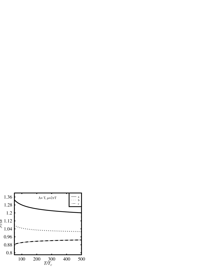
FIG. 5.: The resummed loop expansion of the SU(3) free energy: a) the 1-loop, b) 2-loop and c) the 3-loop level free energy for $m_{T}=0$.

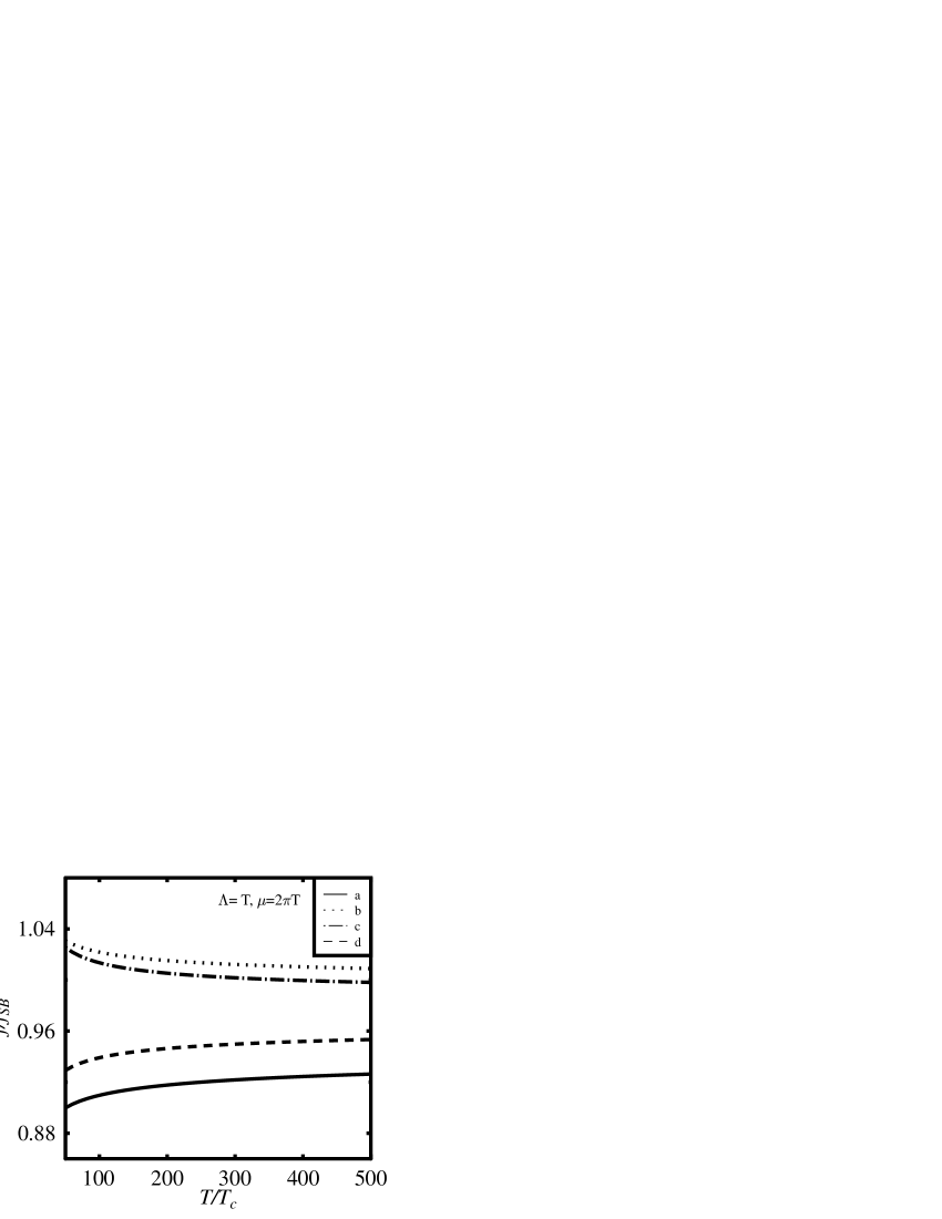
FIG. 6.: The weak coupling expansion of the SU(3) free energy: a, b, c and d are the ${\cal O}(g^{2})$, ${\cal O}(g^{3})$, ${\cal O}(g^{4})$ and ${\cal O}(g^{5})$ level results

First let us investigate the resummed loop expansion for the free energy in the case $m_{T}=0$. The numerical results of the loop expansion are shown in Figure 5. For comparison we have also plotted in Figure 6 the weak coupling expansion for the free energy calculated in [1, 3] which shows the known alternating behaviour in different orders. Compared to this in the resummed loop expansion the contribution of the static modes is larger, but the free energy decreases systematically, contrary to the alternating behaviour of the weak coupling expansion. The 3-loop level resummed free energy if compared to ${\cal O}(g^{5})$ order result differ from it by the amount of a few percent. Finally the effect of massive magnetic modes was studied at 2-loop level and it turns out that the variation of the free energy is about 1% relative to the $m_{T}=0$ case.

VI Summary

The free energy density has been shown in this paper to be rather sensitive to the actual values of the screening masses. This is probably also true for other physical quantities. This gives the motivation for the careful analytical and numerical investigation of these quantities, presented in our paper.

Both numerical Monte-Carlo simulations and investigations of the coupled gap equations show that the magnetic mass of the 3d adjoint Higgs model is very close to the magnetic mass of the pure 3d gauge theory, however, the numerical values of the magnetic mass obtained in these aproaches are different. The 1-loop gap equation approach gives the magnetic mass roughly equal to $0.28g_{3}^{2}$ for BP scheme and $0.38g_{3}^{2}$ for AN scheme, while the numerical lattice simulations give $0.46g_{3}^{2}$. The temperature dependence of the Debye mass was found very close to the leading order result both in the gap equation approach and in the numerical lattice simulations, but the numerical values are again different and equal to $(1.2-1.3)m_{D0}$ for the coupled gap equations ( for $T>100T_{c}$ ) depending on resummation scheme (see Figure 1) and $1.6m_{D0}$ for lattice simulations.

We leave the interpretation of these systematic deviations to a future publication. Acknowledgements: This work was partly supported by the TMR network Finite Temperature Phase Transitions in Particle Physics, EU contract no. ERBFMRX-CT97-0122. P.P. thanks V.P. Nair, O. Philipsen and K. Rummukainen for useful discussions and the organizers of the TFT98 workshop for financial support.

REFERENCES

- [1] C. Zhai and B. Kastening, Phys. Rev. D52 (1995) 7232
- [2] A. Rebhan, Nucl. Phys. B430 (1994) 319
- [3] E. Braaten and A. Nieto, Phys. Rev. D53 (1996) 3421
- [4] B. Kastening, Phys. Rev. D56 (1997) 8107
- [5] A. Linde, Phys. Lett. B96 (1980) 289
- [6] U.M. Heller, F. Karsch and J. Rank, Phys. Lett. B355 (1995) 511
- [7] U.M. Heller, F. Karsch and J. Rank, Phys. Rev. D57 (1998) 1438
-
[8]
W. Buchmüller, Z. Fodor, T. Helbig and D. Walliser, Ann. Phys. (N.Y.) 234 (1994) 260
W. Buchmüller and O. Philipsen, Nucl. Phys. B443 (1995) 47 - [9] G. Alexanian and V.P. Nair, Phys. Lett. B352 (1995) 435
- [10] R. Jackiw and S.-Y. Pi, Phys. Lett. B403 (1997) 297
- [11] F. Eberlein, Two-Loop Gap Equations for the Magnetic Mass, hep-ph/9804460
-
[12]
P. Ginsparg, Nucl. Phys. B170 (1980) 388;
T. Appelquist and R. Pisarski, Phys. Rev. D 23 (1981) 2305;
S. Nadkarni, Phys. Rev. D27 (1983) 917;
K. Kajantie, M. Laine, K. Rummukainen and M. Shaposhnikov, Nucl. Phys. B458 (1996) 90 - [13] P. Arnold and L.G. Yaffe, Phys. Rev. D52 (1995) 7208
- [14] K. Kajantie, M. Laine, K. Rummukainen and M. Shaposhnikov, Nucl. Phys. B503 (1997) 357
- [15] K. Kajantie, M. Laine, J. Peisa, A. Rajantie, K. Rummukainen and M. Shaposhnikov , Phys. Rev. Lett. 79 (1997) 3130
- [16] M. Laine and O. Philipsen, Nucl. Phys. B523 (1998) 267
- [17] D. Karabali and V.P. Nair, Nucl. Phys. B464 (1996) 135; Phys. Lett. (1996) B379 141; Int. J. Mod. Phys. A12 (1997) 1161
- [18] D. Karabali, C. Kim and V.P. Nair, Nucl. Phys. B524 (1998) 661; hep-th/9804132
- [19] A. Patkós, P. Petreczky and Zs. Szép, Eur. Phys. J C5 (1998) 5
- [20] F. Karsch, M. Oevers and P. Petreczky, hep-lat/9807035
- [21] F. Karsch, M. Lütgemeier, A. Patkós and J. Rank, Phys. Lett. B390 (1997) 275
- [22] F. Karsch, A. Patkós and P. Petreczky, Phys. Lett. B401 (1997) 69
- [23] I.T. Drummond, R.R. Horgan, P.V. Landshoff and A. Rebhan, Nucl.Phys. B524 (1998) 579
- [24] C. Bernard, D. Murphy, A. Soni and K. Yee, Nucl. Phys. B (Proc. Suppl.) 17 (1990) 593
- [25] L. Kärkkäinen P. Lacock, D.E. Miller, B. Peterson and T.Reisz, Nucl. Phys. B418 (1994) 3
- [26] S. Nadkarni, Nucl. Phys. B334 (1990) 559
- [27] A. Hart, O. Philipsen, J.D. Stack and M. Tepper, Phys. Lett. B396 (1997) 217
- [28] J. Polónyi and S. Vazquez, Phys. Lett. B240 (1990) 183
- [29] R. Kobes, G. Kunstatter, A. Rebhan, Phys. Rev. Lett. 64 (1990); R. Kobes, G. Kunstatter, A. Rebhan, Nucl. Phys. B355 (1991) 1