Monte Carlo Estimate of Finite Size Effects
in Quark-Gluon Plasma Formation

Abstract

Using lattice simulations of quenched QCD we estimate the finite size effects present when a gluon plasma equilibrates in a slab geometry, i.e., finite width but large transverse dimensions. Significant differences are observed in the free energy density for the slab when compared with bulk behavior. A small shift in the critical temperature is also seen. The free energy required to liberate heavy quarks relative to bulk is measured using Polyakov loops; the additional free energy required is on the order of $30-40~{}MeV$ at $2-3~{}T_{c}$.

I INTRODUCTION

The formation of a quark-gluon plasma in a central heavy ion collision is generally assumed to take place in a coin-shaped region roughly 1 fermi in width, with radius comparable to the radii of the colliding nuclei, which is to say several fermi. While lattice gauge theory has given us information about bulk thermodynamic behavior, finite size effects have up to now been studied using simplified, phenomenological models. We study via lattice gauge theory simulations the behavior of a gluon plasma restricted to a slab geometry, with the longitudinal width much smaller than the transverse directions. This inner region is heated to temperatures above the bulk deconfinement temperature, surrounded by an outer region which is kept at a temperature below the deconfinement temperature, providing confining boundary conditions for the inner region. Details of this work are given in [1].

Measurements of the equilibrium surface tension $\alpha_{0}$ of pure SU(3) lattice gauge theory (quenched lattice QCD) show that the dimensionless ratio $\alpha_{0}/T_{c}^{3}$ is small. For the case of an $N_{s}^{3}\times 4$ lattice, $\alpha_{0}/T_{c}^{3}\approx 0.0292(22)$.[2] A simple estimate of surface tension effects on the transition temperature can be obtained from a simplified model in which only volume and surface terms appear, as in the bag model.[3] Based on these simple considerations, finite size effects due to the surface tension should be small.

Other contributions to finite size effects come from a variety of sources. In the case of systems with non-abelian symmetries, global color invariance produces an additional finite volume effect which will not be considered here. [4][5][6] In general, finite size effects lead to a rounding of the transition. [7] This can be taken into account in the bag model by a Maxwell construction, leading to mixed phases and a broadened critical region. A recent treatment for the quark gluon plasma can be found in [8]. We have attempted to avoid these finite volume effects by making the transverse dimensions large.

II METHODOLOGY

In lattice calculations, finite temperature is introduced by the choice of $N_{t}$, the extent of the lattice in the (Euclidean) temporal direction. The relation of physical temperature $T$ to $N_{t}$ and the lattice spacing $a$ is simply $T=1/{N_{t}a}$. The lattice spacing $a$ implicitly depends on the gauge coupling $\beta=6/g^{2}$ in a way determined by the renormalization group equations. To lowest order in perturbation theory, the relation is given by

$$a\Lambda_{L}=\left({\beta\over{2Nb_{0}}}\right)^{b_{1}/2b_{0}^{2}}exp[-\beta/4Nb_{0}]$$ (1)

where $\Lambda_{L}$ is renormalization group invariant and the renormalization group coefficients $b_{0}$ and $b_{1}$ are given by

$$b_{0}={11N\over{48\pi^{2}}}\ \ ,\ \ b_{1}={34\over 3}\left({N\over{16\pi^{2}}}\right)^{2}$$ (2)

In analyzing our data, we used the renormalization group results given in reference [9], which are determined directly from lattice simulations, and contain non-perturbative information about the renormalization group flow.

By allowing the coupling constant $\beta$ to vary with spatial location, a spatially dependent temperature can be introduced. We have chosen the temperature interface to be sharp, in such a way that the lattice is divided into two spatial regions, one hotter and one colder. The quenched approximation simplifies the role of the cold region, because below $T_{c}$, the dominant excitation at low energies is the scalar glueball. Temperatures near $T_{c}$ are smaller than glueball masses by about a factor of four, so glueballs play no essential role in the thermodynamics, and the pressure in the hadronic phase is essentially zero. We thus expect the slab thermodynamics to be largely insensitive to the precise temperature of the region outside the slab, as long as it is sufficiently low. In full QCD, this insensitivity to the outer temperature would not hold, due to pions. Note that the role of boundary conditions here is quite different from that in bubble nucleation. In that case, both $\beta_{in}$ and $\beta_{out}$ are taken to be near $T_{c}$. [10][11]

The slab is given a fixed lattice width, $w=6a$, rather than of fixed physical width. Since $N_{t}=4$, $wT$ is fixed at $3/2$. At higher temperatures, the width in physical units is somewhat smaller than the longitudinal size of the plasma formation region expected in heavy ion collisions. While the use of equilibrium statistical mechanics to study gluon plasma properties during the early stages of plasma formation may appear suspect, a simple estimate using the Bjorken model [12] shows that when a coin-shaped region of width 1 fermi has expanded to 1.5 fermi, the variation in temperature is only from $0.8T_{0}$ at the center of the coin to $T_{0}$ at its edges.

The free energy density $f$ for the slab is obtained using the standard method [13] of integrating the lattice action with respect to $\beta$. We use a convenient convention for the sign of $f$ that is opposite the usual one. In the bulk case, $f$ is then identical to the pressure $p$.

$${f\over T^{4}}|_{\beta_{out}}^{\beta}=N_{t}^{4}\int_{\beta_{out}}^{\beta}d\beta^{\prime}\left[\langle S\rangle_{T}-\langle S\rangle_{0}\right]$$ (3)

where $S=(1/N)ReTr\ U_{p}$. As in the bulk case, it is necessary to subtract the zero-temperature expectation value from the finite temperature expectation value, in this case using the same pair of $\beta$ values. In general, quantum field theories with boundaries develop divergences that are not present in infinite volume or with periodic boundary conditions. Such divergences would require additional boundary counterterms. Symanzik [14] has shown to all orders in perturbation theory that in the case of $\phi^{4}$ with so-called Schrodinger functional boundary conditions that the theory is finite in perturbation theory after adding all possible boundary counterterms of dimension $d\leq 3$ consistent with the symmetries of the theory. It is generally believed that this result applies as well to all renormalizable field theories and general boundary conditions, but a proof is lacking. Luscher et al. [15] have shown for gauge theories that at one loop no new divergences are introduced by Schrodinger functional boundary conditions. This is consistent with the non-existence of gauge-invariant local fields of dimension $\leq 3$ in pure Yang-Mills theory.

In order to take advantage of the data on bulk thermodynamics provided by the Bielefeld group [9], we worked consistently with lattices of overall size $16^{3}\times 4$. The values used for each subtraction come from $16^{4}$ lattices with identical values of $\beta_{in}$ and $\beta_{out}$. The value of $\beta_{out}$ was held fixed at $5.6$ while $\beta_{in}$ varied from $5.6$ to $6.3$. For comparison, the bulk transition for $N_{t}=4$ occurs at $\beta_{c}(N_{t}=4,N_{s}=16)=5.6908(2)$ $\beta_{c}(N_{t}=4,N_{s}=\infty)=5.6925(5)$. [9]

III FREE ENERGY OF GLUONS

Figure 1 shows the free energy density $f/T^{4}$ versus $T/T_{c}$ compared with the bulk pressure. The free energy in the slab is lower than the bulk value by almost a factor of two at $2T_{c}$. It appears that the slab value is slowly approaching the bulk value, but other behaviors are also possible. Calculations of the finite-temperature contribution to the Casimir effect for a free Bose field contained between two plates show that $f/T^{4}$ has a non-trivial dependence on the dimensionless combination $wT$.[16] [17] It is natural to ask if the corrections to the free energy seen here can be accounted for by the conventional Casimir effect. A straightforward calculation of the free energy of a non-interacting gluon gas confined to a slab shows an increase in the free energy density over the bulk value by a factor of about 1.63 at $wT=3/2$. The Casimir effect cannot explain the reduction of the free energy observed in our simulations.

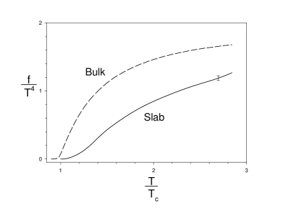
FIG. 1.: Slab free energy compared with bulk pressure.

A consistency check was performed on the surface effects.[18] The free energy density was calculated for a system at $\beta_{in}=6.0$ by performing simulations with $\beta_{in}$ fixed at $6.0$ and $\beta_{out}$ varying from $5.6$ to $6.0$. Combining these results with the bulk data of reference [9] creates a path equivalent to varying $\beta_{in}$ while holding $\beta_{out}$ fixed. For $\beta_{in}=6.0$ and $\beta_{out}=5.6$, this gives $f/T^{4}=0.65\pm 0.04$, to be compared with $f/T^{4}=0.69\pm 0.03$ for the direct calculation. The major source of systematic error lies with the choice of boundary conditions for the slab, here set by $\beta_{out}$. We have estimated the effects of varying $\beta_{out}$ by performing simulations at $\beta_{in}=6.2$ and $\beta_{out}=5.5$ on $16^{3}\times 4$ and $16^{4}$ lattices. These results suggest that lowering $\beta_{out}$ from $5.6$ to $5.5$ reduces the free energy by roughly 10 percent at $\beta_{in}=6.2$.

IV SURFACE TENSION

We define an effective surface tension $\alpha(w,T)$ by

$$f=p-2\alpha(w,T)/w$$ (4)

where the notation $\alpha(w,T)$ recognizes that the surface tension $\alpha$ does depend on the width of the slab and the internal and external temperatures. The factor of $2$ occurs because the slab has two faces. In the limits where $T$ approaches $T_{c}$ and $w$ goes to infinity, this quantity approaches $\alpha_{0}$. Figure 2 shows $\alpha(w,T)/T^{3}$ versus $T/T_{c}$ for $wT=3/2$; representative error bars are shown.

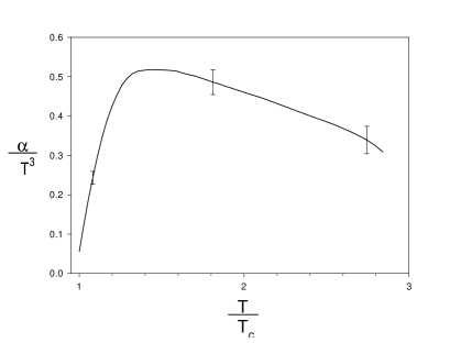
FIG. 2.: Non-equilibrium surface tension versus $T$.

The value at $\beta=5.7$, $0.056\pm 0.002$ is higher than the value $\alpha_{0}=0.0292\pm 0.0022$ given in reference [2]. We attribute this to two effects: in our case $\beta_{out}$ is fixed at 5.6, whereas for equilibrium measurements it is extrapolated to $\beta_{c}$, and our finite value of the width $w$ also acts to increase $\alpha(w,T)$ over the equilibrium value as measured in simulations at large $w$. Away from the bulk critical point, $\alpha/T^{3}$ rises quickly to a peak at about $1.4T_{c}$, and then falls slowly as $T$ increases. A large non-equilibrium surface tension has also been observed in measurements of the equilibrium surface tension, where these effects were obstacles to obtaining $\alpha_{0}$.[18]

V FREE ENERGY OF QUARKS

The Polyakov loop defined by

$$P(\vec{x})=(1/N_{c})Tr~{}{\cal P}\exp\left[i\int^{1/T}_{0}A_{0}(\vec{x},\tau)~{}d\tau\right]$$ (5)

is the order parameter for the deconfinement transition in pure (quenched) gauge theories. In the case of $SU(N)$, there is a global $Z(N)$ symmetry which ensures at low temperature that the expectation value $\langle TrP\rangle$ is $0$. At sufficiently high temperatures, this symmetry is spontaneously broken. The expectation value of the Polyakov loop can also be interpreted in terms of the free energy of an isolated, infinitely heavy quark $F_{Q}$:

$$\left<P(\vec{x})\right>=exp\left[-F_{Q}(\vec{x})/T\right]$$ (6)

In the low-temperature confined phase, $F_{Q}$ is taken to be infinite, whereas in the high temperature phase it is finite. Direct extraction of $F_{Q}$ from computer simulations is problematic, because the expectation value has a multiplicative, $\beta$-dependent ultraviolet divergence. This divergence can be eliminated when comparing bulk expectation values to those in finite geometries. We define

$$\Delta F_{Q}(\vec{x})=-T~{}ln\left[P_{slab}(\vec{x})/P_{bulk}\right]$$ (7)

as the excess free energy required to liberate a heavy quark in the slab geometry relative to bulk quark matter at the same temperature. This technique can also be used in, e.g., a spherical geometry, which is relevant for nucleation. [19][10]

In figure 3, we show the expectation value for the Polyakov loop versus z measured in lattice units for several values of $\beta$. Each curve is normalized by dividing the values of the Polyakov loop by the bulk expectation value at the corresponding value of $\beta$. Error bars are shown only for even values of z.

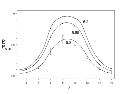
FIG. 3.: Polyakov loop versus $z$.

It is clear that a significant change occurs between $\beta=5.8~{}~{}~{}(T=1.23~{}T_{c})$ and $\beta=5.85~{}~{}~{}(T=1.36~{}T_{c})$. For larger values of $\beta$, $\Delta F_{Q}$ diminishes to a value of approximately $30-40~{}~{}MeV$ in the middle of the slab. In table 1, we list $\beta$, $T$, slab width in fermis, width of the core in fermis, and $\Delta F_{Q}$ in MeV for representative values. The width of the core is calculated by interpolating the Polyakov loop profiles and determining the region where the slab expectation value is greater than 80% of the bulk value. All conversions to physical units are performed by taking the string tension $\sigma$ to be $(425~{}MeV)^{2}$, which implies $T_{c}=254~{}MeV$.[9]

TABLE I.: $\beta$, $T$, slab width in fermis, width of the core in fermis, and $\Delta F_{Q}$ in MeV for representative values.

$\beta$	$T$ (MeV)	w (fm.)	$w_{core}$ (fm.)	$\Delta F_{Q}$ (MeV)
5.8	313	0.95	0	169
5.85	346	0.86	0.40	57
6.0	455	0.65	0.48	41
6.2	624	0.47	0.40	31

VI CONCLUSIONS

There are significant deviations in the slab geometry from bulk behavior and the ideal gas law, arising from a strong non-equilibrium surface-tension. This non-equilibrium surface tension can be an order of magnitude greater than the equilibrium value. Surface tension effects also produce a mild elevation of the apparent critical temperature. Measurement of Polyakov loop expectation values relative to bulk shows that the suppression of heavy quark production due to the slab geometry is small.

There are good reasons to call our result an estimate rather than a calculation. Although lattice gauge theory simulations of bulk behavior can be made arbitrarily accurate in principle, in this case there is some uncertainty in the precise exterior boundary conditions appropriate, and indeed in the applicability of equilibrium thermodynamics at this early stage of quark-gluon plasma formation. However, this seems like the best estimate available now, and further refinements are possible.

We have not yet explored the nature of the phase transition, which will require some care. One interesting possibility is that the order of the transition might change as the width changes. The deconfinement transition in bulk quenched finite temperature QCD is in the universality class of the three-dimensional three-state Potts model, which has a first-order phase transition. As the width of the slab becomes commensurate with the correlation length near $T_{c}$, the phase transition should cross over to the universality class of the two-dimensional three-state Potts model. The two-dimensional three-state Potts model has a second-order phase transition, so it is possible that the order of the transition may change.[20] The correlation length at the bulk transition is known to be large [21], so it is likely that the transverse correlation length in the gluonic sector is much larger in the slab geometry than in bulk, even if crossover does not take place.

The system studied here has some interesting features amenable to theoretical analysis. In the outer region, the Polyakov loop will decay away from the interface as $exp[-\sigma r/T_{out}]$, where $\sigma$ is the string tension. In the inner region, the Debye screening length sets the scale for the Polyakov loop. We are currently working on a theoretical model of this system based on perturbation theory which has these features.

REFERENCES

- [1] Andy Gopie and Michael C. Ogilvie, hep-lat/9803005.
- [2] Y. Iwasaki, K. Kanaya, Leo Kärkkäinen, K. Rummukainen and T. Yoshie, Phys.Rev. D49 , 3540 (1994).
- [3] J. Cleymans, R. Gavai and E. Suhonen, Phys. Rep. 130, 217 (1986).
- [4] K. Redlich and L. Turko, Z. Phys. C5, 201 (1980).
- [5] L. Turko, Phys. Lett. B104, 153 (1981).
- [6] B.S. Skagerstam, Phys. Lett. B133, 419 (1983).
- [7] K. Binder and D.P. Landau, Phys. Rev. B30, 1477 (1984).
- [8] C. Spieles, H. Stöcker, and C. Greiner, Phys. Rev. C57, 908 (1998).
- [9] G. Boyd, J. Engels, F. Karsch, E. Laermann, C. Legeland, M. Lutgemeier and B. Petersson, Nucl. Phys. B469, 419 (1996).
- [10] K. Kajantie, L. Kärkkäinen and K. Rummukainen, Phys. Lett. 286B , 125 (1992).
- [11] S. Huang, J. Potvin and C. Rebbi, Int. J. Mod. Phys. C3 , 931 (1992).
- [12] J. Bjorken, Phys. Rev. D49, 140 (1983).
- [13] J. Engels, J. Fingberg, F. Karsch, D. Miller and M. Weber, Phys. Lett. B252, 625 (1990).
- [14] K. Symanzik in Mathematical Problems in Theoretical Physics, R. Schrader et al., eds., Spinger, New York (1982).
- [15] M. Luscher, R. Narayanan, P. Weisz and U. Wolff, Nucl. Phys. B384, 168 (1992).
- [16] J. Mehra, Physica 37, 145 (1967).
- [17] G. Plunien, B. Müller and W. Greiner, Phys. Rep. 134, 87 (1986).
- [18] S. Huang, J. Potvin, C. Rebbi and S. Sanielevici, Phys. Rev. D42, 2864 (1990); Erratum ibid. D43, 2056 (1991).
- [19] M. Ogilvie, Nucl. Phys. B (Proc. Suppl.) 30, 354 (1993).
- [20] Y. Shnidman and E. Domany, J. Phys. C14, L773 (1981).
- [21] M. Fukugita, M. Okawa and A. Ukawa, Nucl. Phys. B337, 181 (1990).