MADPH-98-1041
NUHEP 501
hep-ph/9809403
September, 1998
Photon-Proton and Photon-Photon Scattering from Nucleon-Nucleon Forward Amplitudes

We show that the data on $\gamma p$ and $\gamma\gamma$ interactions can be derived from the $pp$ and $\bar{p}p$ forward scattering amplitudes using vector meson dominance and the additive quark model. The nucleon–nucleon data are parameterized using a model where high energy cross sections rise with energy as a consequence of the increasing numbers of soft partons populating the colliding particles. We present detailed descriptions of the data on the total and elastic cross sections, the ratio of the real to imaginary part of the forward scattering amplitude, and on the slope of the differential cross sections for $pp$, $\bar{p}p$, $\gamma p$, $\gamma\gamma$, $\gamma p\rightarrow\gamma V$ and $\gamma\gamma\rightarrow V_{i}V_{j}$ reactions, where $V=\rho,\omega,\phi$. We make a wide range of predictions for future HERA and LHC experiments and for $\gamma\gamma$ measurements at LEP.

1 Introduction

We show that the data on $\gamma p$ and $\gamma\gamma$ interactions can be derived from the $pp$ and $\bar{p}p$ forward scattering amplitudes using vector meson dominance (VMD) and the additive quark model. We first show that the data on the total cross section, the slope parameter $B$ and the ratio of the real to imaginary part of the forward scattering amplitude $\rho$ for $pp$ and $\bar{p}p$ interactions, can be nicely described by a model where high energy cross sections rise as a consequence of the increasing numbers of soft partons populating the colliding particles[1]. The differential cross sections for the Tevatron and LHC are predicted. Using this parameterization of the hadronic forward amplitudes, we calculate the photoproduction cross sections, slope and $\rho$ value from VMD and the additive quark model. We then obtain $\gamma\gamma$ cross sections which are again parameter-free, demonstrating the approximate validity of the factorization theorem.

All cross sections will be computed in an eikonal formalism guaranteeing unitarity throughout:

$$\sigma_{\rm tot}(s) = 2\int\,\left[1-e^{-\chi_{{}_{\rm I}}(b,s)}\cos(\chi_{{}_{\rm R}}(b,s))\right]\,d^{2}\vec{b},$$ (1)

Here, $\chi$ is the complex eikonal ( $\chi=\chi_{{}_{\rm R}}+i\chi_{{}_{\rm I}}$) , and $b$ the impact parameter. The even eikonal profile function $\chi^{\rm even}$ receives contributions from quark-quark, quark-gluon and gluon-gluon interactions, and therefore

$$\chi^{\rm even}(s,b) = \chi_{qq}(s,b)+\chi_{qg}(s,b)+\chi_{gg}(s,b)$$ (2)

$$= i\left[\sigma_{qq}(s)W(b;\mu_{qq})+\sigma_{qg}(s)W(b;\sqrt{\mu_{qq}\mu_{gg}})+\sigma_{gg}(s)W(b;\mu_{gg})\right]\,,$$

where $\sigma_{ij}$ is the cross sections of the colliding partons, and $W(b;\mu)$ is the overlap function in impact parameter space, parameterized as the Fourier transform of a dipole form factor. This formalism is identical to the one used in “mini-jet” models, as well as in simulation programs for minimum-bias hadronic interactions such as PYTHIA and SYBILL.

In this model hadrons asymptotically evolve into black disks of partons. The rising cross section, asymptotically associated with gluon-gluon interactions, is simply parameterized by a normalization and energy scale, and two parameters: $\mu_{gg}$ which describes the “area” occupied by gluons in the colliding hadrons, and $J(=1+\epsilon)$. Here, $J$ is defined via the gluonic structure function of the proton, which is assumed to behave as $1/x^{J}$ for small x. It therefore controls the soft gluon content of the proton, and it is meaningful that its value ($\epsilon\simeq 0.05$) is consistent with the one observed in deep inelastic scattering. The introduction of the quark-quark and quark-gluon terms allows us to adequately parameterize the data at all energies, since the “size” of quarks and gluons in the proton can be different. We obtain $\mu_{qq}=0.89$ GeV, and $\mu_{gg}=0.73$ GeV. This indicates that gluons occupy a larger area of the proton than do quarks.

The photoproduction cross sections are then calculated from this parameterization of the hadronic forward amplitudes, assuming vector meson dominance and the additive quark model. To this end , we introduce $P_{\rm had}$, the probability that the photon interacts as a hadron. We will use the value $P_{\rm had}=1/240$ which can be derived from vector meson dominance. Our results show that its value is indeed independent of energy. It is, however, uncertain by 30% because it depends on whether we relate photoproduction to $\pi$-nucleon or nucleon-nucleon data (in other words, $\pi N$ and $NN$ elastic cross sections only satisfy the additive quark model to this accuracy). Subsequently, following reference [2], we obtain $\gamma p$ cross sections from the assumption that, in the spirit of VMD, the photon is a 2 quark state, in contrast with the proton which is a 3 quark state. Using the additive quark model and quark counting, the $\gamma p$ total cross section is obtained from the even eikonal for $pp$ and $\bar{p}p$ by the substitutions:

$$\sigma_{ij} \rightarrow \textstyle\frac{2}{3}\,\sigma_{ij}\;,$$

$$\mu_{i} \rightarrow \sqrt{\textstyle\frac{3}{2}}\,\mu_{i}\,.$$

We will thus produce a parameter-free description of the total photoproduction cross section, the phase of the forward scattering amplitude and the forward slope for $\gamma p\rightarrow Vp$, where $V=\rho,\omega,\phi$. Interestingly, our results on the phase of $Vp\rightarrow Vp$ are in complete agreement with the values derived from Compton scattering results ($\gamma+p\rightarrow\gamma+p$) using dispersion relations. We also calculate the total elastic and differential cross sections for $\gamma p\rightarrow Vp$. This wealth of data is accommodated without discrepancy.

The $\gamma\gamma$ cross sections are derived following the same procedure. We now substitute

$$\sigma_{ij} \rightarrow \textstyle\frac{4}{9}\,\sigma_{ij}\;,$$

$$\mu_{i} \rightarrow \textstyle\frac{3}{2}\,\mu_{i}\;,$$

into the nucleon-nucleon even eikonal, and predict the total cross section and differential cross sections for all reactions $\gamma\gamma\rightarrow V_{i}V_{j}$ at a variety of energies, where $V=\rho,\omega,\phi$.

The high energy $\gamma\gamma$ total cross section [3] have been measured by two experiments at LEP. These measurements yield new information on its high energy behavior at center-of-mass energies in excess of $\sqrt{s}=15$ GeV. However, the two data sets unfortunately disagree. We here point out that our analysis nicely accommodates the L3 measurements. The analysis is sufficiently restrictive to exclude the preliminary OPAL results [4]. It is interesting to note that the small eikonal found in our model by fitting n-n data—as shown later— enforces naturally the validity of the factorization theorem,

$$\frac{\sigma_{pp}}{\sigma_{\gamma p}}=\frac{\sigma_{\gamma p}}{\sigma_{\gamma\gamma}},$$ (3)

a result independent of the details of our model. We find that the L3 data satisfy the factorization theorem whereas the preliminary OPAL data do not. VMD and factorization are sufficient to prevent one from adjusting $P_{\rm had}$, or any other parameters, to change this conclusion.

An interesting theoretical issue emerges when it is noticed that we applied the additive quark model to the full hadronic eikonal, not just to the quark subprocesses in Eq. 2. This was not a choice—we found that the data clearly enforced it. For example, if we do not apply the quark counting rules to the gluon-gluon subprocess, the model fails to reproduce the forward slope of the $\gamma p\rightarrow\gamma V$ reactions, as well as the ratio of the imaginary to real part of the $\gamma p\rightarrow\gamma p$ forward amplitude. It, in fact, fails dramatically. This result may suggest either a static structure of the nucleon where the gluons cluster around the original valence quarks, as in the valon model [6], or a dynamic picture in which the gluons are associated with the interaction of the valence quarks during the hadronic collision. This picture is reinforced by correlation measurements between quarks and gluons, derived from the observation of multiple parton final state in hadron collisions [7].

We further emphasize the energy-independence of $P_{\rm had}$. In other words, the shapes of the total cross sections for $\gamma p$ and $\gamma\gamma$ reactions as a function of energy are completely fixed by the shape of the nucleon-nucleon data.

2 High Energy $\bar{p}p$ and $pp$ Scattering

In this Section, we will discuss high energy $\bar{p}p$ and $pp$ scattering. In Section 2.1, we will discuss the theory of our QCD-inspired eikonal and its implementation in fitting the experimental data for $\sigma_{\rm tot},\ \rho$ and $B$ to determine the parameters of the model.

In Section 2.2, we will compare the experimental data for the elastic scattering cross section, $\sigma_{\rm elastic}$ as a function of energy with our predictions.

In Section 2.3, we will show predictions for differential elastic scattering at $\sqrt{s}=1800$ GeV, compared to experimental data, and finally, a prediction for the differential elastic scattering at the LHC.

2.1 The Fit to High Energy $\bar{p}p$ and $pp$ Scattering Data

We will fit all available high energy forward scattering data above 15 GeV, using both $\bar{p}p$ and $pp$, for

1. $\sigma_{\rm tot}$, the total cross section,

2. $\rho$, the ratio of the real to the imaginary part of the forward scattering amplitude,

3. $B$, the logarithmic slope of the differential elastic scattering cross section in the forward direction.

We insist that our QCD-inspired model satisfies:

1. crossing symmetry, i.e., be either even or odd under the transformation $E\rightarrow-E$, where E is the laboratory energy. This allows us to simultaneously describe $\bar{p}p$ and $pp$ scattering.

2. unitarity. We will use an eikonal formalism to guarantee this.

3. analyticity. We need this to calculate the phase of the forward scattering amplitude and hence, the $\rho$ value.

4. the Froissart bound. Asymptotically, we expect that the total cross section will rise as $(\log s)^{2}$.

The formalism needed to derive $\sigma_{\rm tot}$, $\rho$ and $B$ from an eikonal are given in Appendix A, in sections A.1.1, A.1.5 and A.1.6, in eqns. (A8), (A14) and (A20), respectively. Details on the analyticity are given in Ap pendices B.3.1 and B.4. The even portion (under crossing) of our QCD-inspired eikonal, as noted in eq. (2), contains quark-quark, quark-glue and glue-glue components, of which the glue-glue portion dominates at high energy. A detailed parameterization of this portion is given in Appendix B.1, sections B.1.1 and B.1.1.2. The even eikonal we finally use is given in eq. (B23).

We show in Appendix B.1.1.1 that the Froissart bound is satisfied by our glue-glue interaction, and that, asymptotically, the cross section is given by

$$\sigma_{tot}=2\pi\left(\frac{\epsilon}{\mu_{gg}}\right)^{2}\log^{2}\frac{s}{s_{0}},$$ (4)

as seen in eq. (B14). The parameter $\epsilon$ is defined via the gluonic structure of the proton, which is assumed to behave as $1/x^{1+\epsilon}$, for small $x$. The mass $\mu_{gg}$ describes the area occupied by the gluons in the colliding hadrons. Both are fitted from experiment, with $\epsilon\approx 0.05$ and $\mu_{gg}\approx 0.73$ GeV. These two parameters, along with the threshold mass $m_{0}\approx 0.6$ GeV and the strength of the glue-glue interaction, $C_{gg}$, are all that is required to specify the glue-glue interaction. These 4 parameters dominate the high energy behavior of the nucleon-nucleon cross section and are the critical elements of our fit.

The quark-quark and quark-glue portions are discussed in Appendices B.2 and B.3, and are simulated by a constant strength $C$, a Regge descending trajectory strength $C_{\rm Regge\ even}$, a strength $C_{\rm qg\ log}$ for a log term, an energy scale $\sqrt{s}_{0}$ for the log term and a quark size $\mu_{qq}$, as detailed in eq. (B22) in Appendix B.3.1. We show how to make the even eikonal analytic in section B.3.1. Details of the odd eikonal are given in Appendix B.4, and the odd eikonal, which contains two parameters, a strength $C_{\rm odd}$ and a size $\mu_{\rm odd}$, is given in eq. (B24).

In all, 11 parameters are used in the theoretical model. The low energy region, for $\sqrt{s}\raisebox{-2.58334pt}{\ $\stackrel{{\scriptstyle<}}{{\sim}}$\ }25$ GeV, where the differences between $\bar{p}p$ and $pp$ scattering are substantial, largely determine the 7 parameters necessary to fit the odd eikonal and the quark-quark and the quark-glue portions of the even eikonal. Thus, they largely decouple from the high energy behavior, which depends on only 4 of these quantities. Hence, for $\sqrt{s}\raisebox{-2.58334pt}{\ $\stackrel{{\scriptstyle>}}{{\sim}}$\ }25$ GeV, where there is little difference between $\bar{p}p$ and $pp$ scattering, we really need only 4 parameters for our model.

We use in the fit all of the highest energy cross sections available, (E710[8], CDF[9] and the unpublished Tevatron value[10]) which anchor the upper end of our cross section curves. The results of the fit are shown in Figs. 1, 2 and 3. The total cross sections $\sigma_{\rm tot}$ for $\bar{p}p$ (dotted line and circles) and for $pp$ (solid line and squares) are plotted against $\sqrt{s}$, the cms energy, in Fig. 1.

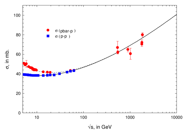
Figure 1: The total cross section $\sigma_{\rm tot}$, in mb vs. $\sqrt{s}$, in GeV, for $pp$ and $\bar{p}p$ scattering. The solid line and squares are for $pp$ and the dotted line and circles are for $\bar{p}p$.

The $\rho$ values (the ratio of the real to the imaginary portion of the forward scattering amplitude) are plotted in Fig. 2 using the same conventions,

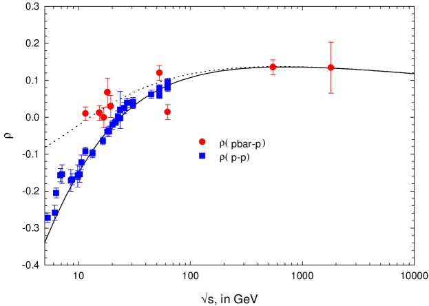
Figure 2: The ratio of the real to imaginary part of the forward scattering amplitude, $\rho$ vs. $\sqrt{s}$, in GeV, for $pp$ and $\bar{p}p$ scattering. The solid line and squares are for $pp$ and the dotted line and circles are for $\bar{p}p$.

and the nuclear slope B values are similarly plotted in Fig. 3.

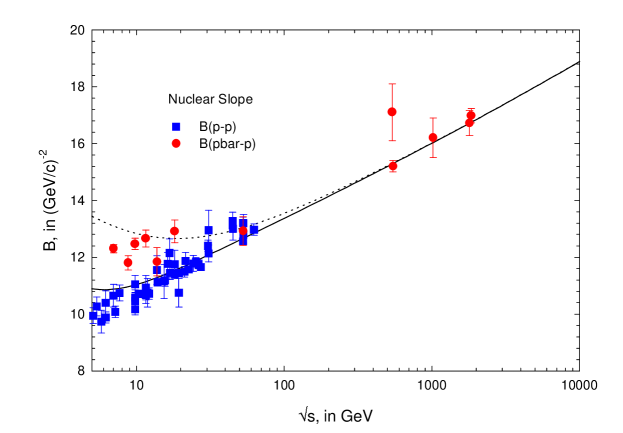
Figure 3: The nuclear slope parameter B, in (GeV/c)^-2 vs. $\sqrt{s}$, in GeV, for elastic $pp$ and $p\bar{p}$ scattering. The solid line and squares are for $pp$ and the dotted line and circles are for $\bar{p}p$.

It can be seen from these figures that we have a quite satisfactory description of all 3 quantities, for both $\bar{p}p$ and $pp$ scattering. The $\chi^{2}$ of the fit is reasonably good (considering the large spreads in the experimental data—in $B$, in particular, as well as the discrepancies in t he highest energy cross sections), giving a $\chi^{2}$ of 130.3, where 75 was expected. The cross section fit of Fig. 1 splits the difference between the values at $\sqrt{s}=1800$ GeV. From Fig. 2, we note that the fit to $\rho$ is anchored at $\sqrt{s}=550$ GeV by the very accurate measurement[12] of UA4/2 and passes through the E710 point[11].

The statistical uncertainty of the fitted parameters is such that at 25 GeV, the cross section predictions are statistically uncertain to $\approx 1.3$%, at 500 GeV are uncertain to $\approx 1.6$% and at 2000 GeV are uncertain to $\approx 2.5$% .

2.2 Predictions for Elastic Scattering Cross Sections

We now have all the parameters needed to specify our eikonal. In Fig. 4 we have plotted our prediction for the elastic cross section $\sigma_{\rm elastic}$, in mb vs. the cms energy $\sqrt{s}$, in GeV, along with the available data for both $\bar{p}p$ and $pp$. The agreement is excellent.

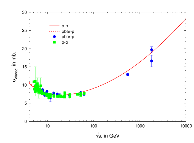
Figure 4: Elastic scattering cross sections, $\sigma_{\rm elastic}$, in mb vs. $\sqrt{s}$, in GeV, for $pp$ and $p\bar{p}$ scattering. The solid line and squares are for $pp$ and the dotted line and circles are for $\bar{p}p$.

We note that $\sigma_{\rm elastic}$ is rising more sharply with energy than does the total cross section $\sigma_{\rm to}$. Comparing Fig. 1 with Fig. 4, we see that the ratio of the elastic to total cross section is rising significantly with energy. The ratio is, of course, bounded by the value for the black disk[14, 15], i.e., 0.5, as the energy goes to infinity.

2.3 Predictions for $\bar{p}p$ Elastic Differential Scattering Cross Sections at 1800 GeV

¿From eq. (A.1.4), we can now calculate $\frac{ds}{dt}$, the elastic differential cross section as a function of $|t|$, for various values of $\sqrt{s}$. The calculated differential cross section at the Tevatron ($\sqrt{s}=1800$ GeV) is shown in Fig. 5 and compared with the experimental data from E710[13]. The agreement over 4 decades is striking.

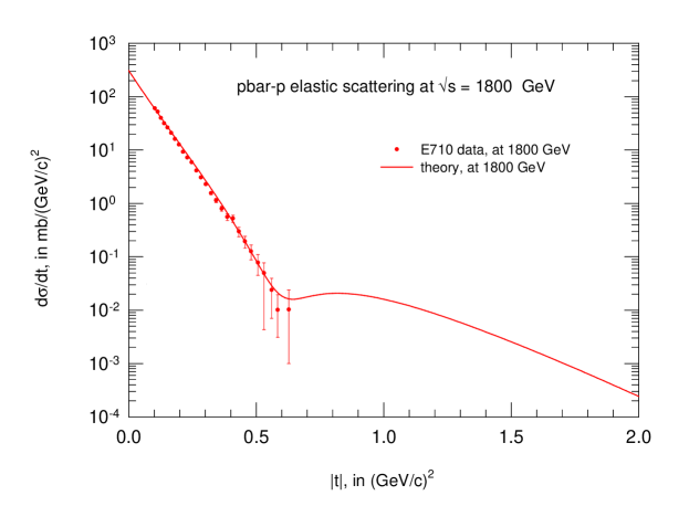
Figure 5: The elastic differential scattering cross section $\frac{d\sigma}{dt}$, in mb/(GeV/c)² vs. $|t|$, in (GeV/c)², for the reaction $\bar{p}p\rightarrow\bar{p}p$ at $\sqrt{s}=1800$ GeV. The solid curve is the prediction at the Tevatron Collider and the data points are from E710.

2.4 Predictions for $\bar{p}p$ at the LHC

With the parameters we obtained from our fit, we predict the total cross section at the LHC (14 TeV) as $\sigma_{\rm tot}=108.0\pm 3.4$ mb, where the error is due to the statistical errors of the fitting parameters.

Our prediction for the differential cross section for $\sqrt{s}=14$ TeV, the energy of the LHC, is plotted in Fig. 6.

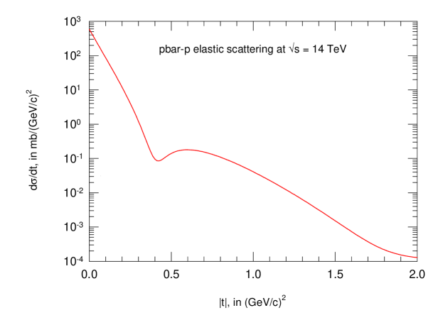
Figure 6: The predicted elastic differential scattering cross section $\frac{d\sigma}{dt}$, in mb/(GeV/c)² vs. $|t|$, in (GeV/c)², for the reaction $\bar{p}p\rightarrow\bar{p}p$ at $\sqrt{s}=14$ TeV, at the LHC.

It will be a challenge to the LHC to measure this cross section and to confirm the predicted structure in $|t|$. In particular, at small $|t|$, we predict that the curvature parameter $C$ (see Appendix A.1.7 for details) is negative. For energies much lower than 1800 GeV, the observed curvature has been measured as positive. For 1800 GeV, we see from Fig. 5 that the curvature parameter $C$ is compatible with being zero. Block and Cahn[14, 15] had pointed out that they expected the curvature to go through zero near the Tevatron energy an d that it should become negative thereafter. Basically, the argument is that experimentally, the curvature for the then available energies was positive. However, it was expected that the scattering asymptotically would approach that of a sharp disk. The curvature of a (gray) sharp disk[14, 15] is always negative, $C=-R^{4}/192$, where $R$ is the radius of the disk. Thus, the curvature had to pass through zero as the energy increased. They called ‘asymptopia’ the energy region (energies much larger than the Tevatron Collider) where the scattering approached that of a sharp disk .

3 $\gamma p$ Reactions

In our model, when the photon interacts strongly, it behaves like a two quark system. Taking the quark model literally, the eikonal for $\gamma p$ scattering is obtained by rewriting the even eikonal with the substitutions

$$\sigma_{ij} \rightarrow \textstyle\frac{2}{3}\,\sigma_{ij}\;,$$

$$\mu_{i} \rightarrow \sqrt{\textstyle\frac{3}{2}}\,\mu_{i}\,,$$ (5)

as

$$\chi^{\gamma p}(s,b) = i\left[\frac{2}{3}\sigma_{qq}(s)W\left(b;\sqrt{\frac{3}{2}}\mu_{qq}\right)+\frac{2}{3}\sigma_{qg}(s)W\left(b;\sqrt{\frac{3}{2}}\sqrt{\mu_{qq}\mu_{gg}}\right)\right.$$ (6)

$$\qquad\left.+\frac{2}{3}\sigma_{gg}(s)W\left(b;\sqrt{\frac{3}{2}}\mu_{gg}\right)\right]\,.$$

3.1 $\gamma p$ Total Cross Section Prediction

Using vector dominance and the $\gamma p$ eikonal of eq. (6), we can now write, using eq. (A8),

$$\sigma_{\rm tot}^{\gamma p}(s)= 2P_{\rm had}\int\,\left[1-e^{-{\chi_{{}_{\rm I}}}^{\gamma p}(b,s)}\cos({\chi_{{}_{\rm R}}}^{\gamma p}(b,s))\right]\,d^{2}\vec{b},$$ (7)

where $P_{\rm had}$ is the probability that a photon will interact as a hadron. We will use the value $P_{\rm had}=1/240$, which is found by fitting the low energy $\gamma p$ data. This value is very close to that derived from VDM. Using (see Table XXXV, p.393 of ref. [16]) $\frac{f_{\rho}^{2}}{4\pi}=2.2$, $\frac{f_{\omega}^{2}}{4\pi}=23.6$ and $\frac{f_{\phi}^{2}}{4\pi}=18.4$, we find $\Sigma_{V}\frac{4\pi\alpha}{f_{V}^{2}}=1/249$, where $V=\rho,\omega\phi$.

With all eikonal parameters fixed from our nucleon-nucleon fits and our choice of $P_{\rm had}=1/240$, we can now calculate $\sigma_{\rm tot}^{\gamma p}(s)$. Our prediction is given in Fig. 7,

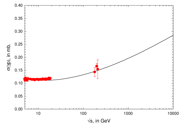
Figure 7: The total cross section, $\sigma_{\rm tot}$, in mb vs. $\sqrt{s}$, in GeV, for $\gamma p$ scattering. The solid curve is the predicted total cross section.

where $\sigma_{\rm tot}^{\gamma p}(s)$ is plotted against the cms energy. The fit reproduces the rising cross section for $\gamma p$, using parameters fixed by nucleon-nucleon scattering. We comment here that this prediction only uses the 9 parameters of the even eikonal, of which but 4 are important in the upper energy region. The accuracy of our predictions are $\approx 1.5\%$, from the statistical uncertainty in our eikonal parameters.

3.2 ‘Elastic’ $\gamma p$ Scattering

We consider as ‘elastic’ scattering the three vector reactions

$$\gamma+p \rightarrow \rho_{\rm virtual}+p\rightarrow\rho+p$$

$$\gamma+p \rightarrow \omega_{\rm virtual}+p\rightarrow\omega+p$$

$$\gamma+p \rightarrow \phi_{\rm virtual}+p\rightarrow\phi+p,$$ (8)

where the photon virtually materializes as a vector meson, which then elastically scatters off of the proton. The strengths of these reactions is $\approx\alpha$, the fine-structure constant, times a strong interaction cross section. The true elastic cross section is given by Compton scattering on the proton, $\gamma+p\rightarrow\gamma+p$, which we can visualize as

$$\gamma+p \rightarrow \rho_{\rm virtual}+p\rightarrow\rho+p\rightarrow\gamma+p$$

$$\gamma+p \rightarrow \omega_{\rm virtual}+p\rightarrow\omega+p\rightarrow\gamma+p$$

$$\gamma+p \rightarrow \phi_{\rm virtual}+p\rightarrow\phi+p\rightarrow\gamma+p,$$ (9)

is clearly $\alpha^{2}$ times a strong interaction cross section, and hence is much smaller than ‘elastic’ scattering of eq. (8). Thus, we justify using eq. (7) to calculate the total cross section which we compare with experiment, since only reactions with a photon in the final state (down by $\approx\alpha$) are neglected.

3.2.1 Predictions of $\rho$ and $B$ for ‘Elastic’ $\gamma p$ Reactions

Using the philosophy of ‘elastic’ scattering expressed in eq. (8), and eqns. (A14) and (A20), we can immediately write

$$\rho(s) = \frac{{\rm Re}\left\{i(\int 1-e^{i\chi^{\gamma p}(b,s)})\,d^{2}\vec{b}\right\}}{{\rm Im}\left\{i(\int(1-e^{i\chi^{\gamma p}(b,s)})\,d^{2}\vec{b}\right\}},$$ (10)

and

$$B=\frac{1}{2}\frac{\int\left(1-e^{i\chi^{\gamma p}(b,s)}\right)\,b^{2}\,\,d^{2}\vec{b}}{\int\left(1-e^{i\chi^{\gamma p}(b,s)}\right)\,\,d^{2}\vec{b}}.$$ (11)

We see from eqns. (10) and (11) that the predictions for both $\rho$ and the slope $B$ are free of any $P_{\rm had}$ factors and hence are independent of normalization—thus being the same for either $\rho p,\ \omega p$ or $\phi p$ final states.

In Fig. 8 the value of $\rho$ from eq. (10) is the solid curve, plotted as a function of $\sqrt{s}$. Damashek and Gilman[17] calculated the $\rho$ value for Compton scattering on the proton, using dispersion relations, i.e., the true elastic scattering reaction for photon-proton scattering. We compare this calculation, the dotted line in Fig. 8, with our prediction of $\rho$ (the solid line). The agreement is so close that we had to move the two curves apart so that they may be viewed more clearly—this gives us confidence in our approach.

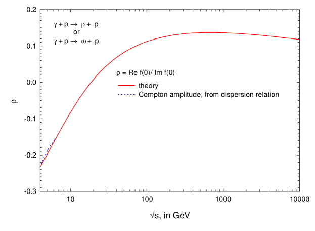
Figure 8: The solid curve is the predicted ratio of the real to imaginary part of the forward scattering amplitude for the ‘elastic’ reactions , $\gamma+p\rightarrow V_{i}+p$ scattering amplitude, where $V_{i}$ is $\rho^{0}$, $\omega^{0}$ or $\phi^{0}$ vs. $\sqrt{s}$, in GeV. The dotted curve is ratio of the real to imaginary part of the forward scattering amplitude for Compton scattering[17], $\gamma+p\rightarrow\gamma+p$, found from dispersion relations. It has been slightly displaced from the solid curve for clarity in viewing.

In Fig. 9 the solid curve is our prediction for the slope $B$ against the energy $\sqrt{s}$. The available experimental data for ‘elastic’ $\rho p$ and $\omega p$ final states are also plotted. Again, the agreement of theory and experiment is quite satisfactory.

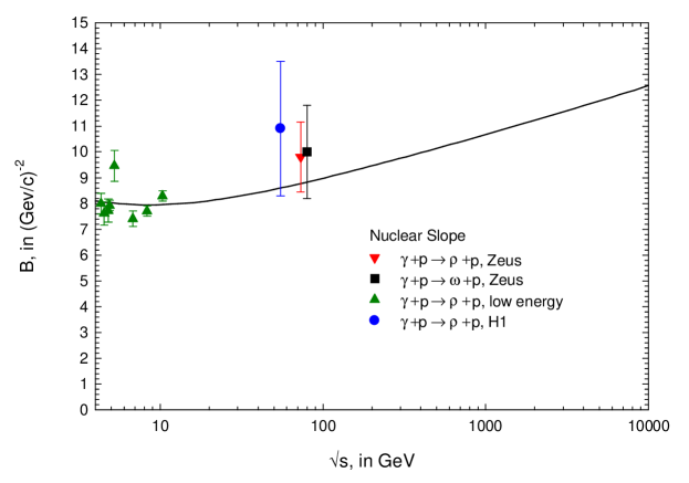
Figure 9: The predicted nuclear slope parameter B, in (GeV/c)^-2 vs. $\sqrt{s}$, in GeV, for the ‘elastic’ reaction $\gamma+p\rightarrow V_{i}+p$, where $V_{i}$ is $\rho^{0}$, $\omega$ or $\phi$ scattering. The solid curve is the prediction. For the reaction $\gamma+p\rightarrow\rho^{0}+p$, the inverted triangles are the Zeus data, the circles are the H1 data and the triangles are the low energy data. For the reaction $\gamma+p\rightarrow\omega+p$, the squares are the Zeus data.

We note that the predictions of $\rho$ and $B$ are very critical to our analysis. We have assumed that in some manner, the gluons are “attached” to the quarks—when we have a two quark system, such as the photon, the factors of 2/3 times a cross section and $\sqrt{3/2}$ times a $\mu$ of eq. (5) in the even eikonal of eq. (6) are the same for glue-glue as for quark-quark. If we relax this assumption, and only use these factors in the quark, then we get sharp disagreement with our predicted $\rho$ value—being considerably larger than the Compton value. This is further exacerbated in the predictions for $B$, with slopes from 11 (at 5 GeV) to 16 (GeV/c)^-2 (at 80 GeV), which are much larger than the experimental values. We stress that these conclusions are independent of our choice of $P_{\rm had}$. Thus, our model clearly has dynamical consequences whi ch will be discussed in detail later.

3.2.2 Predictions of $\sigma_{\rm elastic}$ and $\frac{d\sigma}{dt}$ for ‘Elastic’ $\gamma p$ Reactions

To find the elastic cross sections $\sigma_{\rm elastic}^{Vp}$ and differential cross sections $d\sigma^{Vp}/dt$ as a function of energy, using eq. (A9), we write

$$\sigma_{\rm elastic}^{Vp}(s) = P_{\rm had}^{Vp}\int\left|1-e^{i\chi^{\gamma p}(b,s)}\right|^{2}\,d^{2}\vec{b},$$ (12)

where $P_{\rm had}^{Vp}$ is the appropriate probability for a photon to turn into $V$, where $V=\rho,\ \omega$ or $\phi$, respectively.

Similarly, the differential scattering cross section is, using eq. (A13), given by

$$\frac{d\sigma^{Vp}}{dt}(s,t)=\frac{P_{\rm had}^{Vp}}{4\pi}\left|\int J_{0}(qb)(1-e^{i\chi^{\gamma p}(b,s)})\,d^{2}\vec{b}\,\right|^{2},$$ (13)

where $t=-q^{2}$. The same factors $P_{\rm had}^{Vp}$ are used in eq. (13) as in eq. (12).

Since we normalize the experimental data to the elastic cross section found with $\chi^{\gamma p}$, and not to $\frac{1}{2}(\sigma^{\pi^{+}}_{\rm elastic}+\sigma^{\pi^{-}}_{\rm elastic})$, we find that must multiply all $\frac{f_{V}^{2}}{4\pi}$ by 1.65. Hence, our effective coupling s are

$$\frac{{f_{\rho}^{2}}_{\rm eff}}{4\pi}=3.6,\quad\frac{{f_{\omega}^{2}}_{\rm eff}}{4\pi}=38.9\quad\rm{and}\quad\frac{{f_{\phi}^{2}}_{\rm eff}}{4\pi}=30.4.$$ (14)

Thus, we define the $P_{\rm had}^{Vp}$ in eq. (13) and eq. (12) as

$$P_{\rm had}^{Vp}=\frac{4\pi\alpha}{{f_{V}^{2}}_{\rm eff}}.$$ (15)

In Fig. 10, we show our prediction for the ‘elastic’ reaction $\gamma+p\rightarrow\rho^{0}+p$, where we plot the elastic cross section $\sigma_{\rm elastic}^{\rho p}(s)$ against the cms energy. The solid curve is the predicted cross section, the squares are Zeus data, the circles are H 1 data and the inverted triangles the low energy data.

     

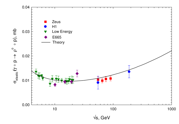
Figure 10: The ‘elastic’ photoproduction cross section, $\sigma_{\rm elastic}$, in mb vs. $\sqrt{s}$, in GeV, for the reaction $\gamma+p\rightarrow\rho^{0}+p$. The solid curve is the predicted cross section, the squares are Zeus data, the circles are H1 data and the inverted tri angles the low energy data.

In Fig. 11, we show our prediction for the ‘elastic‘ reaction $\gamma+p\rightarrow\omega+p$. The solid curve is the predicted cross section, the circles are Zeus data and the squares are the low energy data.

     

Figure 11: The ‘elastic’ photoproduction cross section, $\sigma_{\rm elastic}$, in $\mu$b vs. $\sqrt{s}$, in GeV, for the reaction $\gamma+p\rightarrow\omega+p$. The solid curve is the predicted cross section, the circles are Zeus data and the squares are the low energy data.

The agreement of Figs. (10) and (11) is very good, lending further support to the model.

The predicted differential cross sections, $d\sigma/dt$, for the ‘elastic’ reactions $\gamma+p\rightarrow\rho^{0}+p$, $\gamma+p\rightarrow\omega+p$ and $\gamma+p\rightarrow\phi+p$, for diverse energies, are plotted in Figs. 12, 13 and 14, respec tively. The agreement, in absolute normalization and shape, of the predicted differential scattering cross sections with the experimental data for all three light mesons for all available energies reinforces even more our confidence in our model of $\gamma p$ scattering.

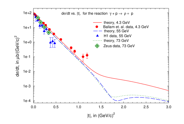
Figure 12: The predicted differential scattering cross section $\frac{d\sigma}{dt}$, in $\mu$b/(GeV/c)² vs. $|t|$, in (GeV/c)², for the ‘elastic’ reaction $\gamma+p\rightarrow\rho^{0}+p$. The solid curve and the circles (Ballam et al. data) are at $\sqrt{s}$= 4.3 GeV, the dashed curve and triangles (H1 data) are at $\sqrt{s}$= 55 GeV and the dotted curve and diamonds are at $\sqrt{s}$= 73 GeV (Zeus data).

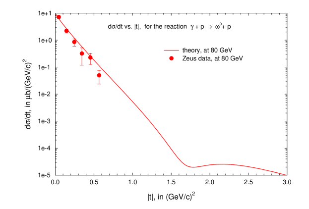
Figure 13: The predicted differential scattering cross section $\frac{d\sigma}{dt}$, in $\mu$b/(GeV/c)² vs. $|t|$, in (GeV/c)², for the ‘elastic’ reaction $\gamma+p\rightarrow\omega+p$, at $\sqrt{s}$=80 GeV. The circles are the Zeus data.

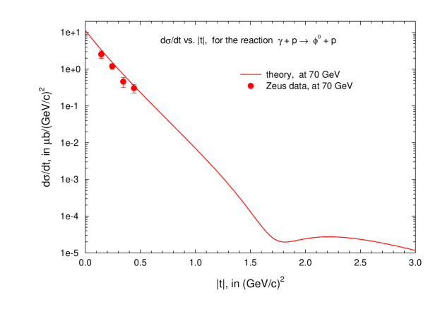
Figure 14: The predicted differential scattering cross section $\frac{d\sigma}{dt}$, in $\mu$b/(GeV/c)² vs. $|t|$, in (GeV/c)², for the ‘elastic’ reaction $\gamma+p\rightarrow\phi+p$, at $\sqrt{s}$=70 GeV. The circles are the Zeus data.

3.3 How Large is the $\rho$, $\omega$ and $\phi$ Contribution?

We sum all of our predictions for the elastic vector interactions for $\rho$, $\omega$ and $\phi$ and divide this sum by the ratio of $\sigma_{\rm elastic}/\sigma_{\rm tot}$ (obtained from $\chi^{\gamma p}$, using eq. (A8) and eq. (A9)). We call this quantity the total vector meson con tribution. In Fig. 15, we compare this to the total $\gamma p$ cross section. We find that the fraction of the total cross section for $\gamma p$ reactions that is contributed by the three light vector mesons ($\rho$, $\omega$ and $\phi$) is $\approx 0.60$. The remaining 40% could, in the spirit of VMD, be made up of heavier vector meson states, or perhaps could be continuum states, or, indeed, a mixture of both.

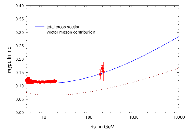
Figure 15: The dotted curve is the prediction for the total vector meson photoproduction cross section, in mb, i.e., the sum of $\gamma+p\rightarrow\rho^{0}+p$, $\gamma+p\rightarrow\omega+p$ and $\gamma+p\rightarrow\phi+p$, divided by the ratio of elastic to total cross se ction (see text). For comparison, we also show the solid line and the data which are the predicted and experimental total photoproduction cross sections on protons, in mb, vs. $\sqrt{s}$ in GeV.

4 $\gamma\gamma$ Interactions

In this Section, we consider $\gamma\gamma$ interactions. As we did for $\gamma p$ interactions, we will take the eikonal $\chi^{\gamma p}(s,b)$ and again multiply every cross section by 2/3 and multiply each $\mu$ by $\sqrt{3/2}$. Thus, we have

$$\chi^{\gamma\gamma}(s,b) = i\left[\frac{4}{9}\sigma_{qq}(s)W\left(b;\frac{3}{2}\mu_{qq}\right)+\frac{4}{9}\sigma_{qg}(s)W\left(b;\frac{3}{2}\sqrt{\mu_{qq}\mu_{gg}}\right)\right.$$ (16)

$$\qquad\left.+\frac{4}{9}\sigma_{gg}(s)W\left(b;\frac{3}{2}\mu_{gg}\right)\right]\,.$$

4.1 $\gamma\gamma$ Total Cross Section Prediction

Again, using vector dominance and the $\gamma\gamma$ eikonal of eq. (16), we can now write, using eq. (A8),

$$\sigma_{\rm tot}^{\gamma\gamma}(s)= 2\left((P_{\rm had}\right)^{2}\int\,\left[1-e^{-{\chi_{{}_{\rm I}}}^{\gamma\gamma}(b,s)}\cos({\chi_{{}_{\rm R}}}^{\gamma p}(b,s))\right]\,d^{2}\vec{b},$$ (17)

where, again, $P_{\rm had}=1/240$ is the probability that a photon will interact as a hadron. In Fig. 16 we plot our prediction for $\sigma_{\rm tot}^{\gamma\gamma}(s)$ as a function of the cms energy and compare it to the various sets of experimental data. It is clear that VMD selects the L3 and casts doubt on the preliminary OPAL results[3].

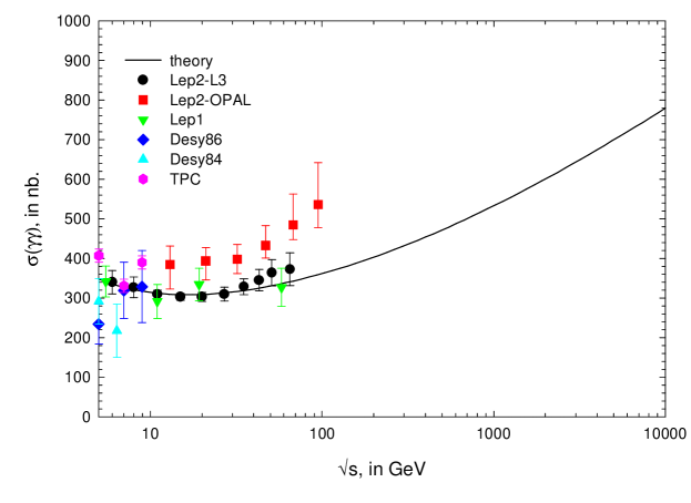
Figure 16: The predicted total cross section, $\sigma_{\rm tot}$, in nb vs. $\sqrt{s}$, in GeV, for $\gamma\gamma$ scattering. The data sources are indicated in the legend.

4.2 ‘Elastic’ $\gamma\gamma$ Reactions

In this Section, we make prediction for ‘elastic’ $\gamma\gamma$ reactions, in which both photons turn into vector mesons, and then elastically scatter off each other, i.e., $\gamma+\gamma\rightarrow V_{i}+V_{j}\rightarrow V_{i}+V_{j}$, where $V_{i},V_{j}=\rho,\,\omega,\,\phi$. We consider here the 6 reactions

$$\gamma+\gamma\rightarrow\rho^{0}+\rho^{0},$$ (18)

$$\gamma+\gamma\rightarrow\rho^{0}+\omega,$$ (19)

$$\gamma+\gamma\rightarrow\rho^{0}+\phi,$$ (20)

$$\gamma+\gamma\rightarrow\omega+\omega,$$ (21)

$$\gamma+\gamma\rightarrow\omega+\phi,$$ (22)

$$\gamma+\gamma\rightarrow\phi+\phi.$$ (23)

There currently exist no data for such reactions, but hopefully, there will be in the foreseeable future—perhaps these predictions will be useful for experimental planning.

4.2.1 ‘Elastic’ $\gamma\gamma$ Cross Sections

To find the total ‘elastic’ scattering cross sections, we invoke eq. (A9) of Appendix A.1.2, using the eikonal $\chi^{\gamma\gamma}$ of eq. (16), multiplied by the factors $P_{had}^{V_{i}}P_{had}^{V_{j}}$, i.e., $\sigma_{\rm el}(s)$ as

$$\sigma_{\rm elastic}^{\gamma\gamma}(s) = 2P_{had}^{V_{i}}P_{had}^{V_{j}}\int\left|1-e^{i\chi^{\gamma\gamma}(b,s)}\right|^{2}\,d^{2}\vec{b},\qquad{\rm if\ }i\neq j,$$ (24)

$$= \phantom{2}P_{had}^{V_{i}}P_{had}^{V_{j}}\int\left|1-e^{i\chi^{\gamma\gamma}(b,s)}\right|^{2}\,d^{2}\vec{b},\qquad{\rm if\ }i=j.$$ (25)

The factor of 2 in eq. (24), where there are unlike mesons in the final state, takes into account, for example, that either photon in eq. (19) could turn into a $\rho^{0}$. In eqns. (24) and (25), the factor $P_{\rm had}^{V_{i}}=\frac{4\pi\alpha}{{f_{V_{i}}^{2}}_{\rm eff}},\ V_{i}=\rho,\ \omega,\ \phi$, where, from eq. (14), $\frac{{f_{\rho}^{2}}_{\rm eff}}{4\pi}=3.6,\ \frac{{f_{\omega}^{2}}_{\rm eff}}{4\pi}=38.9,$ and $\frac{{f_{\phi}^{2}}_{\rm eff}}{4\pi}=30.4$.

We show in Fig. 17 the predicted cross section for reaction (18), in Fig. 18 for reactions (19) and (20) and finally, in Fig. 19, for reactions (21), (22) and (23), as a function of $\sqrt{s}$.

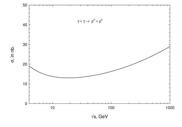
Figure 17: The predicted cross section in nb vs. $\sqrt{s}$, in GeV, for the ‘elastic’ reaction $\gamma+\gamma\rightarrow\rho^{0}+\rho^{0}$.

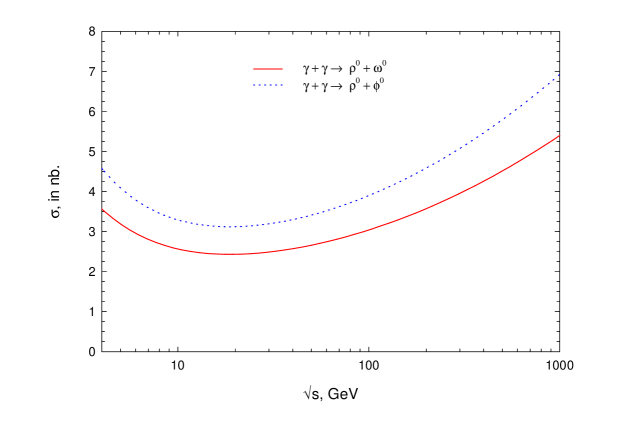
Figure 18: The predicted cross sections in nb vs. $\sqrt{s}$, in GeV, for $\gamma\gamma$ ‘elastic’ reactions. The solid curve is for the reaction $\gamma+\gamma\rightarrow\rho^{0}+\omega$ and the dotted curve for $\gamma+\gamma\rightarrow\rho^{0}+\phi$.

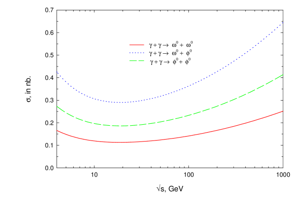
Figure 19: The predicted cross sections in nb vs. $\sqrt{s}$, in GeV, for $\gamma\gamma$ ‘elastic’ reactions. The solid curve is for the reaction $\gamma+\gamma\rightarrow\omega+\omega$, the dotted curve for $\gamma+\gamma\rightarrow\omega+\phi$ and the dashed curve is f or $\gamma+\gamma\rightarrow\phi+\phi$.

4.2.2 Slope Parameters $B$

Using eq. (A20) and the eikonal $\chi^{\gamma\gamma}$, we predict the nuclear slope parameter for the ‘elastic’ reaction of eqns. (18)–(23), as a function of energy. Of course, the slopes are the same for all elastic $\gamma\gamma$ reactions. The predicted slopes B, a s a function of $\sqrt{s}$, are shown in Fig. 20.

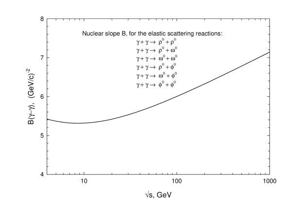
Figure 20: The predicted nuclear slope parameter B, in (GeV/c)^-2 vs. $\sqrt{s}$, in GeV, for the ‘elastic ’ $\gamma\gamma$ reactions $\gamma+\gamma\rightarrow\rho^{0}+\rho^{0}$, $\gamma+\gamma\rightarrow\rho^{0}+\omega$, $\gamma+\gamma\rightarrow\omega^{0}+\omega^{0}$, $\gamma+\gamma\rightarrow\rho^{0}+\phi$, $\gamma+\gamma\rightarrow\omega+\phi$ and$\gamma+\gamma\rightarrow\phi+\phi$.

4.2.3 Differential Cross Sections

Using eq. (A13) and $\chi^{\gamma\gamma}$ of eq. (16), we can write

$$\frac{d\sigma}{dt}(s,t) = 2P_{had}^{V_{i}}P_{had}^{V_{j}}\frac{1}{4\pi}\left|\int J_{0}(qb)(1-e^{i\chi^{\gamma\gamma}(b,s)})\,d^{2}\vec{b}\,\right|^{2},\qquad{\rm if\ }i\neq j,$$ (26)

$$= \phantom{2}P_{had}^{V_{i}}P_{had}^{V_{j}}\frac{1}{4\pi}\left|\int J_{0}(qb)(1-e^{i\chi^{\gamma\gamma}(b,s)})\,d^{2}\vec{b}\,\right|^{2},\qquad{\rm if\ }i=j,$$ (27)

where $t=-q^{2}$. The factor of 2 in eq. (26), where there are unlike mesons in the final state, again takes into account, for example, that either photon in eq. (19) could turn into a $\rho^{0}$. In eqns. (26) and (27), the factor $P_{\rm had}^{V_{i}}=\frac{4\pi\ alpha}{{f_{V_{i}}^{2}}_{\rm eff}},\ V_{i}=\rho,\ \omega,\ \phi$, where, from eq. (14), $\frac{{f_{\rho}^{2}}_{\rm eff}}{4\pi}=3.6,\ \frac{{f_{\omega}^{2}}_{\rm eff}}{4\pi}=38.9,$ and $\frac{{f_{\phi}^{2}}_{\rm eff}}{4\pi}=30.4$.

In Fig. 21 we show the predicted differential scattering cross section $\frac{d\sigma}{dt}$ as a function of $|t|$ for the ‘elastic’ $\gamma\gamma$ reactions of eqns. (18), (19), and (21), at $\sqrt{s}$=5 GeV. The solid curve is for the reaction $\gamma+\gamma\rightarrow\rho^{0}+\rho^{0}$, the dotted curve for $\gamma+\gamma\rightarrow\rho^{0}+\omega$ and the dashed curve for $\gamma+\gamma\rightarrow\omega+\omega$.

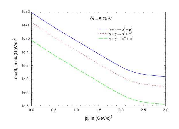
Figure 21: The predicted differential scattering cross section $\frac{d\sigma}{dt}$, in nb/(GeV/c)² vs. $|t|$, in (GeV/c)², for the ‘elastic’ $\gamma\gamma$ reactions, at $\sqrt{s}$=5 GeV. The solid curve is for the reaction $\gamma+\gamma\rightarrow\rho^{0}+\rho^{0}$, the d otted curve for $\gamma+\gamma\rightarrow\rho+\omega$ and the dashed curve for $\gamma+\gamma\rightarrow\omega+\omega$.

In Fig. 22 we show the predicted differential scattering cross section $\frac{d\sigma}{dt}$ for the ‘elastic’ $\gamma\gamma$ reactions of eqns. (20), (22), and (23), at $\sqrt{s}$=5 GeV. The solid curve is for the reaction $\gamma+\gamma\rightarrow\rho^{0}+\rho^{0}$, the dotted curve for $\gamma+\gamma\rightarrow\rho^{0}+\omega$ and the dashed curve for $\gamma+\gamma\rightarrow\omega+\omega$.

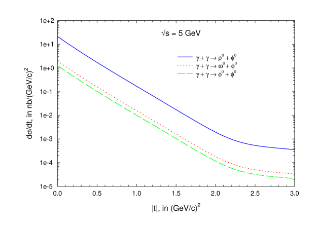
Figure 22: The predicted differential scattering cross section $\frac{d\sigma}{dt}$, in nb/(GeV/c)² vs. $|t|$, in (GeV/c)², for the ‘elastic’ $\gamma\gamma$ reactions, at $\sqrt{s}$=5 GeV. The solid curve is for the reaction $\gamma+\gamma\rightarrow\rho^{0}+\phi$, the dot ted curve for $\gamma+\gamma\rightarrow\omega+\phi$ and the dashed curve for $\gamma+\gamma\rightarrow\phi+\phi$.

In Fig. 23 we show the predicted differential scattering cross section $\frac{d\sigma}{dt}$ for the ‘elastic’ $\gamma\gamma$ reactions of eqns. (18), (19), and (21), at $\sqrt{s}$=20 GeV. The solid curve is for the reaction $\gamma+\gamma\rightarrow\rho^{0}+\rho^{0}$, the dotted curve for $\gamma+\gamma\rightarrow\rho^{0}+\omega$ and the dashed curve for $\gamma+\gamma\rightarrow\omega+\omega$.

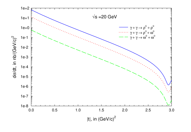
Figure 23: The predicted differential scattering cross section $\frac{d\sigma}{dt}$, in nb/(GeV/c)² vs. $|t|$, in (GeV/c)², for the ‘elastic’ $\gamma\gamma$ reactions, at $\sqrt{s}$=20 GeV. The solid curve is for the reaction $\gamma+\gamma\rightarrow\rho^{0}+\rho^{0}$, the dotted curve for $\gamma+\gamma\rightarrow\rho^{0}+\omega$ and the dashed curve for $\gamma+\gamma\rightarrow\omega+\omega$.

In Fig. 24 we show the predicted differential scattering cross section $\frac{d\sigma}{dt}$ for the ‘elastic’ $\gamma\gamma$ reactions of eqns. (20), (22), and (23), at $\sqrt{s}$=20 GeV. The solid curve is for the reaction $\gamma+\gamma\rightarrow\rho^{0}+\rho^{0}$, the dotted curve for $\gamma+\gamma\rightarrow\rho^{0}+\omega$ and the dashed curve for $\gamma+\gamma\rightarrow\omega+\omega$.

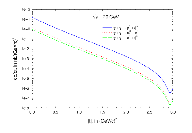
Figure 24: The predicted differential scattering cross section $\frac{d\sigma}{dt}$, in nb/(GeV/c)² vs. $|t|$, in (GeV/c)², for the ‘elastic’ $\gamma\gamma$ reactions, at $\sqrt{s}$=20 GeV. The solid curve is for the reaction $\gamma+\gamma\rightarrow\rho^{0}+\phi^{0}$, the dotted curve for $\gamma+\gamma\rightarrow\omega^{0}+\phi^{0}$ and the dashed curve for $\gamma+\gamma\rightarrow\phi^{0}+\phi^{0}$.

In Fig. 25 we show the predicted differential scattering cross section $\frac{d\sigma}{dt}$ for the ‘elastic’ $\gamma\gamma$ reactions of eqns. (18), (19), and (21), at $\sqrt{s}$=70 GeV. The solid curve is for the reaction $\gamma+\gamma\rightarrow\rho^{0}+\rho^{0}$, the dotted curve for $\gamma+\gamma\rightarrow\rho^{0}+\omega^{0}$ and the dashed curve for $\gamma+\gamma\rightarrow\omega^{0}+\omega^{0}$.

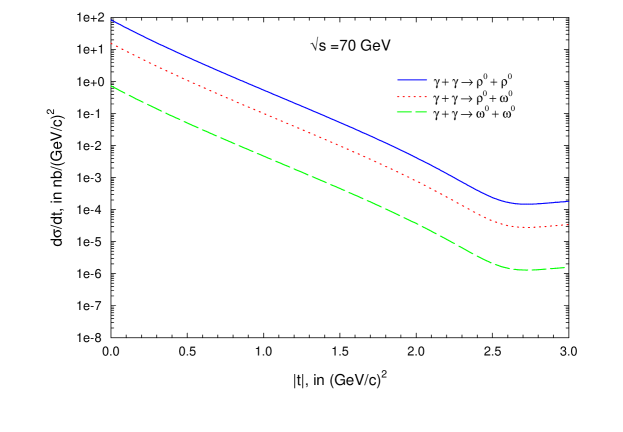
Figure 25: The predicted differential scattering cross section $\frac{d\sigma}{dt}$, in nb/(GeV/c)² vs. $|t|$, in (GeV/c)², for the ‘elastic’ $\gamma\gamma$ reactions, at $\sqrt{s}$=70 GeV. The solid curve is for the reaction $\gamma+\gamma\rightarrow\rho^{0}+\rho^{0}$, the dotted curve for $\gamma+\gamma\rightarrow\rho^{0}+\omega^{0}$ and the dashed curve for $\gamma+\gamma\rightarrow\omega^{0}+\omega^{0}$.

In Fig. 26 we show the predicted differential scattering cross section $\frac{d\sigma}{dt}$ for the ‘elastic’ $\gamma\gamma$ reactions of eqns. (20), (22), and (23), at $\sqrt{s}$=20 GeV. The solid curve is for the reaction $\gamma+\gamma\rightarrow\rho^{0}+\rho^{0}$, the dotted curve for $\gamma+\gamma\rightarrow\rho^{0}+\omega$ and the dashed curve for $\gamma+\gamma\rightarrow\omega+\omega$.

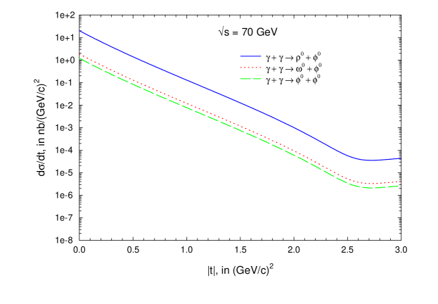
Figure 26: The predicted differential scattering cross section $\frac{d\sigma}{dt}$, in nb/(GeV/c)² vs. $|t|$, in (GeV/c)², for the ‘elastic’ $\gamma\gamma$ reactions, at $\sqrt{s}$=70 GeV. The solid curve is for the reaction $\gamma+\gamma\rightarrow\rho^{0}+\phi$, the dotted curve for $\gamma+\gamma\rightarrow\omega+\phi$ and the dashed curve for $\gamma+\gamma\rightarrow\phi+\phi$.

It would be most interesting to be able to measure the predicted $|t|$ structure shown in these differential cross section curves.

5 Summary and Conclusions

Our conclusions for the total cross section for $\gamma p$ and $\gamma\gamma$ are summarized in Fig. 27. In order to scale nucleon-nucleon, $\gamma p$ and $\gamma\gamma$ cross sections to a common curve, we have multiplied the $\gamma p$ cross sections by $1/P_{\rm had}$ (=240) and the $\gamma\gamma$ cross sections by $(1/P_{\rm had})^{2}$ (=240²). The nucleon-nucleon calculation is made using the even eikonal. For clarity, we have not included the Opal $\gamma\gamma$ experimental data. Basically, both the data and our theory approximately satisfy factorization, with

$$\frac{\sigma_{\rm tot}^{\rm nn-even}}{\sigma_{\rm tot}^{\gamma p}}=\frac{\sigma_{\rm tot}^{\gamma p}}{\sigma_{\rm tot}^{\gamma\gamma}},$$ (28)

an immediate consequence of the eikonal being small in the energy region considered (up to $\approx 2$ TeV). The small eikonal we find is consistent with the Tevatron energy not yet being in ‘asymptopia’.

All data are in agreement with our QCD-inspired eikonal model, which requires that we use the even eikonal. When appropriate factors of 2/3 (for quark counting) are introduced, and an energy independent factor $P_{\rm had}=1/240$ is introduced, we have a natural explanation of $\gamma p$ interacti ons. Finally, when we again introduce another factor of 2/3, and the factor $P_{\rm had}^{2}=\frac{1}{(240^{2})}$, we can explain the total $\gamma\gamma$ cross section, agreeing with the L3 data and disagreeing the Opal results. We stress that the $\gamma p$ and the $\gamma\gamma$ experimental data are consistent with both $P_{\rm had}$ being energy independent and the factorization theorem of eq. (28).

We show that VMD, combined with quark counting, fits all available ‘elastic’ $\gamma p$ data. It even predicts correctly the phase of the forward scattering amplitude for true Compton scattering, $\gamma+p\rightarrow\gamma+p$. Our theory allows us to calculate that the three light vector meson s, $\rho$, $\omega$ and $\phi$, account for about 60% of the total $\gamma p$ cross section.

Finally, there are also dynamical consequences of our phenomenological model. We see that the gluons are carried along with the quarks, since when we link our 2/3 factors exclusively to the quark composition of our eikonal, we get strong disagreement with the measured nuclear slope parameters $B$ for $\gamma p$ ‘elastic’ interactions, as well as disagreement between the $\rho$ values that we predict for ‘elastic’ scattering (such as $\gamma+p\rightarrow\rho^{0}+p$) and the dispersion relation calculation[17] for Compton scattering on a proton, $\gamma+p\rightarrow\gamma+p$.

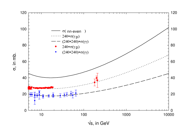
Figure 27: The solid curve is the fitted total cross section for nucleon-nucleon scattering, using the even eikonal . The dotted curve is the predicted total cross section for $\gamma p$ scattering multiplied by $1/P_{\rm had}$ (=240). The circles are the $\gamma p$ data multiplied by $1/P_{\rm had}$. The dashed curve is the predicted total cross section for $\gamma\gamma$ scattering multiplied by $(1/P_{\rm had})^{2}$ (=240*240). The squares are $\gamma\gamma$ total cross section data multiplied by $(1/P_{\rm had})^{2}$.

Appendix A Eikonal Formulation

In order to ensure unitarity, we utilize an eikonal formalism, evaluating the eikonal in the two-dimensional transverse impact parameter space $\vec{b}$. We introduce two eikonals, $\chi^{\rm even}(b,s)$ and $\chi^{\rm odd}(b,s)$, even and odd under crossing, respectively (where the proton labora tory energy ${\rm E}\rightarrow-{\rm E}$), which are both complex and real analytic. In terms of the even and odd eikonals, the eikonals we require for $pp$ and $\bar{p}p$ scattering are given by

$$\chi_{pp}(b,s) = \chi^{\rm even}(b,s)-\chi^{\rm odd}(b,s)$$

$$\chi_{\bar{p}p}(b,s) = \chi^{\rm even}(b,s)+\chi^{\rm odd}(b,s).$$ (A1)

This work largely follows the procedures and conventions used by Block and Cahn[14]. In terms of the c.m. scattering amplitude $f_{\rm c.m.}$, the c.m. differential elastic scattering cross section $\frac{d\sigma}{d\Omega_{\rm c.m.}}(\theta)$, the invariant differential elastic scattering distribution $\frac{d\sigma}{dt}$ and the total cross section $\sigma_{\rm tot}$ are given by

$$\frac{d\sigma}{d\Omega_{\rm c.m.}}(\theta) = \left|f_{\rm c.m.}\right|^{2},$$ (A2)

$$\frac{d\sigma}{dt} = \frac{\pi}{k^{2}}\left|f_{\rm c.m.}\right|^{2},$$ (A3)

$$\sigma_{\rm tot} = \frac{4\pi}{k}{\rm Im}f_{\rm c.m.}(\theta=0),$$ (A4)

where $k$ is the c.m. system momentum, $\theta$ is the c.m. system scattering angle and $t=-2k^{2}(1-\cos\theta)$ is the invariant four-momentum transfer. Let $a(b,s)$ be the scattering amplitude in impact parameter space. The c.m. scattering amplitude[14] is given by

$$f_{\rm c.m.}(s,t)=\frac{k}{\pi}\int\,e^{i\vec{q}\cdot\vec{b}}a(b,s)\,d^{2}\vec{b},$$ (A5)

where $d^{2}\vec{b}=2\pi b\,db$, and $\vec{q}$ is a two-dimensional vector in impact parameter space $\vec{b}$ such that $q^{2}=-t$. Let the eikonal $\chi(b,s)$ be complex, such that

$$\chi(b,s)=\chi_{{}_{\rm R}}(b,s)+i\chi_{{}_{\rm I}}(b,s).$$ (A6)

We define our eikonal $\chi(b,s)$ so that $a(b,s)$, the (complex) scattering amplitude in impact parameter space $b$, is given by

$$a(b,s) = \frac{i}{2}\left(1-e^{i\chi(b,s)}\right)$$ (A7)

$$= \frac{i}{2}\left(1-e^{-\chi_{{}_{\rm I}}(b,s)+i\chi_{{}_{\rm R}}(b,s)}\right).$$

A.1 Forward Scattering Parameters and Cross Sections

We now calculate the forward scattering parameters and various cross sections, using the above eikonal formulation in impact parameter space.

A.1.1 Total Cross Section $\sigma_{\rm tot}(s)$

Using the optical theorem, the total cross section $\sigma_{\rm tot}(s)$ is given by

$$\sigma_{\rm tot}(s) = \frac{4\pi}{k}{\rm Im}\,f_{\rm c.m.}(s,0)$$ (A8)

$$= 4\int\,{\rm Im}\,a(b,s)\,d^{2}\vec{b}$$

$$= 2\int\,\left[1-e^{-\chi_{{}_{\rm I}}(b,s)}\cos(\chi_{{}_{\rm R}}(b,s))\right]\,d^{2}\vec{b},$$

where in eq. (A8), we used eq. (A5) evaluated in the forward direction ($t=0$) and substituted eq. (A7) to evaluate the total cross section in terms of the eikonal $\chi(b,s)$.

A.1.2 Elastic Scattering Cross Section $\sigma_{\rm el}(s)$

¿From eq. (A3), we can evaluate the elastic scattering cross section $\sigma_{\rm el}(s)$ as

$$\sigma_{\rm elastic}(s) = \frac{\pi}{k^{2}}\int\,|f_{\rm c.m.}(s,t)|^{2}\,dt$$ (A9)

$$= \frac{1}{k^{2}}\int\,|f_{\rm c.m.}(s,t)|^{2}\,d^{2}\vec{q}$$

$$= \frac{1}{\pi^{2}}\int\int\int e^{i\vec{q}\cdot(\vec{b}-\vec{b^{\prime}})}a(b,s)a^{*}(b^{\prime},s)\,d^{2}\vec{q}\,d^{2}\vec{b}\,d^{2}\vec{b^{\prime}}$$

$$= \frac{(2\pi)^{2}}{\pi^{2}}\int\int a(b,s)a^{*}(b^{\prime},s)\delta^{2}(\vec{b}-\vec{b^{\prime}})\,d^{2}\vec{q}\,d^{2}\vec{b}$$

$$= 4\int|a(b,s)|^{2}\,d^{2}\vec{b}$$

$$= \int\left|1-e^{-\chi_{{}_{\rm I}}(b,s)+i\chi_{{}_{\rm R}}(b,s)}\right|^{2}\,d^{2}\vec{b}.$$

A.1.3 Inelastic Cross Section $\sigma_{\rm in}(s)$

Thus, using eq. (A8) and eq. (A9), the inelastic cross section, defined as $\sigma_{\rm tot}(s)-\sigma_{\rm elastic}(s)$, is given by

$$\sigma_{\rm inelastic}(s)=\int\,\left\{1-e^{-2\chi_{{}_{\rm I}}(b,s)}\right\}\,d^{2}\vec{b}.$$ (A10)

A.1.4 Differential Elastic Scattering Cross Section $\frac{d\sigma}{dt}(s,t)$

A convenient way of calculating the differential elastic scattering cross section of eq. (A.1.4) is to note that an alternative way to write eq. (A5) is to introduce an integral representation of $J_{0}$ (see eq. (9.1.18), ref. [19]),

$$J_{0}(z)=\frac{1}{2\pi}\int_{0}^{2\pi}\,e^{iz\cos\phi}\,d\phi.$$ (A11)

We can then rewrite eq. (A5) as

$$f_{\rm c.m.}(s,t)=2k\int_{0}^{\infty}\,J_{0}(qb)\,a(b,s)b\,db=\frac{k}{\pi}\int\,J_{0}(qb)\,a(b,s)\,d^{2}\vec{b}.$$ (A12)

Finally, using eq. (A12) and eq. (A3), we now write the differential scattering cross section as

$$\frac{d\sigma}{dt}(s,t)=\frac{1}{4\pi}\left|\int J_{0}(qb)(1-e^{-\chi_{{}_{\rm I}}(b,s)+i\chi_{{}_{\rm R}}(b,s)})\,d^{2}\vec{b}\,\right|^{2},$$ (A13)

a more convenient computational form.

A.1.5 $\rho(s)$

To calculate $\rho$, the ratio of the real to the imaginary portion of the forward nuclear scattering amplitude, we write

$$\rho(s) = \frac{{\rm Re}f_{\rm c.m.}(s,0)}{{\rm Im}f_{\rm c.m.}(s,0)}$$ (A14)

$$= \frac{{\rm Re}\left\{i(\int 1-e^{-\chi_{{}_{\rm I}}(b,s)+i\chi_{{}_{\rm R}}(b,s)})\,d^{2}\vec{b}\right\}}{{\rm Im}\left\{i(\int(1-e^{-\chi_{{}_{\rm I}}(b,s)+i\chi_{{}_{\rm R}}(b,s)})\,d^{2}\vec{b}\right\}}.$$

A.1.6 Nuclear Slope Parameter $B$

The nuclear slope parameter $B$ is defined as

$$B(s)=\frac{d}{dt}\left[\ln\frac{d\sigma}{dt}(s,t)\right]_{t=0}.$$ (A15)

Beginning with eq. (A5),

$$f_{\rm c.m.}(s,t)\propto\int\,e^{i\vec{q}\cdot\vec{b}}a(b,s)\,d^{2}\vec{b},$$ (A16)

we expand the exponential about $q=0$ to get

$$f_{\rm c.m.}(s,t)\propto\int[1+i\vec{q}\cdot\vec{b}-\frac{1}{2}(\vec{q}\cdot\vec{b})^{2}+\cdots]a(b,s)\,d^{2}\vec{b}$$ (A17)

With this expansion and the definition of $B$ in eq. (A15), we can eventually write the general expression for $B$ as

$$B=\frac{{\rm Re}\left\{\int_{0}^{\infty}\,db\,b\,a(b,s)\int_{0}^{\infty}\,db\,b^{3}a^{*}(b,s)\right\}}{2\left|\int_{0}^{\infty}\,db\,b\,a(b,s)\right|^{2}}.$$ (A18)

If the phase of $a(b,s)$ is independent of b (this is the case when we either have a factorizable eikonal or an eikonal with a constant phase), eq. (A18) reduces to the more tractable expression

$$B=\frac{\int_{0}^{\infty}\,db\,b^{3}a(b,s)}{2\int_{0}^{\infty}\,db\,b\,a(b,s)}=\frac{\int\,b^{2}a(b,s)\,d^{2}\vec{b}}{2\int\,a(b,s)\,d^{2}\vec{b}}.$$ (A19)

We note from eq. (A19) that $B$ measures the size of the proton, i.e., $B$ is one-half the average value of the square of the impact parameter $b$, weighted by $a(b,s).$ Again, introducing the eikonal into eq. (A19), we find

$$B=\frac{1}{2}\frac{\int\left(1-e^{-\chi_{{}_{\rm I}}(b,s)+i\chi_{{}_{\rm R}}(b,s)}\right)\,b^{2}\,\,d^{2}\vec{b}}{\int\left(1-e^{-\chi_{{}_{\rm I}}(b,s)+i\chi_{{}_{\rm R}}(b,s)}\right)\,\,d^{2}\vec{b}},$$ (A20)

which we use to compute $B$.

A.1.7 The Curvature Parameter $C$

The $t$ dependence of the elastic differential cross section is described at small $|t|$ as

$$\frac{d\sigma}{dt}(s,t) = \left|\frac{d\sigma}{dt}(s,t)\right|_{t=0}e^{Bt+Ct^{2}+\cdots}$$ (A21)

$$= \left|\frac{d\sigma}{dt}(s,t)\right|_{t=0}\left[1+Bt+\left(\frac{B^{2}}{2}+C\right)t^{2}+\cdots\right].$$

We state, without proof, that the curvature parameter $C$ is given[14] by

$$C(s) = \frac{1}{32}\frac{\int\left(1-e^{-\chi_{{}_{\rm I}}(b,s)+i\chi_{{}_{\rm R}}(b,s)}\right)b^{4}\,d^{2}\vec{b}}{\int\left(1-e^{-\chi_{{}_{\rm I}}(b,s)+i\chi_{{}_{\rm R}}(b,s)}\right)\,d^{2}\vec{b}}$$ (A22)

$$\qquad-\frac{1}{16}\left[\frac{\int\left(1-e^{-\chi_{{}_{\rm I}}(b,s)+i\chi_{{}_{\rm R}}(b,s)}\right)b^{2}\,d^{2}\vec{b}}{\int\left(1-e^{-\chi_{{}_{\rm I}}(b,s)+i\chi_{{}_{\rm R}}(b,s)}\right)\,d^{2}\vec{b}}\right]^{2},$$

where it was again assumed that the phase of the eikonal is independent of $b$ (see eq. (4.45) of ref. [14]). From eq. (A22), we see that the curvature $C$ can be positive, negative or zero, whereas the nuclear slope parameter, from eq. (A20), must be positive.

Appendix B QCD-Inspired Eikonal

B.1 Even Eikonal

The even QCD-Inspired eikonal $\chi_{\rm even}$ is given by the sum of three contributions, glue-glue, quark-glue and quark-quark, which are individually factorizable into a product of a cross section $\sigma(s)$ times an impact parameter space distribution function $W(b\,;\mu)$, i.e.,:

$$\chi^{\rm even}(s,b) = \chi_{\rm gg}(s,b)+\chi_{\rm qg}(s,b)+\chi_{\rm qq}(s,b)$$ (B1)

$$= i\left[\sigma_{\rm gg}(s)W(b\,;\mu_{\rm gg})+\sigma_{\rm qg}(s)W(b\,;\sqrt{\mu_{\rm qq}\mu_{\rm gg}})+\sigma_{\rm qq}(s)W(b\,;\mu_{\rm qq})\right],$$

where the impact parameter space distribution function

$$W(b\,;\mu)=\frac{\mu^{2}}{96\pi}(\mu b)^{3}K_{3}(\mu b)$$ (B2)

is normalized so that

$$\int W(b\,;\mu)d^{2}\vec{b}=1.$$ (B3)

Hence, the $\sigma$’s in eq. (B1) have the dimensions of a cross section.

The factor $i$ is inserted in eq. (B1) since the high energy eikonal is largely imaginary (the $\rho$ value for nucleon-nucleon scattering is rather small).

As a consequence of both factorization and the normalization chosen for the $W(b\,;\mu)$, it should be noted that

$$\int\chi^{\rm even}(s,b)\,d^{2}\vec{b}=i\left[\sigma_{\rm gg}(s)+\sigma_{\rm qg}(s)+\sigma_{\rm qq}(s)\right],$$ (B4)

so that, using eq. (A8) for small $\chi$,

$$\sigma_{\rm tot}^{\rm even}(s)=2\,{\rm Im}\left\{i\left[\sigma_{\rm gg}(s)+\sigma_{\rm qg}(s)+\sigma_{\rm qq}(s)\right]\right\}.$$ (B5)

In eq. (B1), the inverse sizes (in impact parameter space) $\mu_{\rm gg}$ and $\mu_{\rm gg}$ are to be fit by experiment, whereas the quark-gluon inverse size is taken as $\sqrt{\mu_{\rm qq}\mu_{\rm gg}}$.

B.1.1 The $\sigma_{\rm gg}$ Contribution

Modeling the glue-glue interaction after QCD, we write the cross section $\sigma_{\rm gg}(s)$ in eq. (B1) as

$$\sigma_{\rm gg}(s)=C_{\rm gg}N_{\rm g}^{2}\int\Sigma_{\rm gg}\theta(\hat{s}-m_{0}^{2})F_{\rm gg}\left(x_{1}x_{2}=\frac{\hat{s}}{s}\right)\,d\left(\frac{\hat{s}}{s}\right),$$ (B6)

where

$$\Sigma_{\rm gg}=\frac{9\pi\alpha_{s}^{2}}{m_{0}^{2}}.$$ (B7)

The normalization constant $C_{\rm gg}$ and the threshold $m_{0}$ are to be fitted by experiment (in practice, the threshold is taken as $m_{0}=0.6$ GeV and the strong coupling constant $\alpha_{s}$ is fixed at 0.5). The constant $N_{\rm g}$ in eq. (B6) is given by $N_{\rm g}=\frac{3}{2}\frac{(5-\epsilon)(4-\epsilon)(3-\epsilon)(2-\epsilon)(1-\epsilon)}{5!}$. Using the gluon structure function

$$f_{\rm g}(x)=3\frac{(1-x)^{5}}{x^{1+\epsilon}},$$ (B8)

we can now write the function $F_{\rm gg}$ in eq. (B6) as

$$F_{\rm gg}=\int\int f_{\rm g}(x_{1})f_{\rm g}(x_{2})\delta(x_{1}x_{2}=\tau)\,dx_{1}\,dx_{2}.$$ (B9)

After carrying out the integrations, we can now explicitly express $\sigma_{\rm gg}(s)$ as a function of $s$. The parameter $\epsilon$ in eq. (B8) is to be fitted by experiment (in practice, we fix it at 0.05).

B.1.1.1 High Energy Behavior of $\sigma_{\rm gg}(s)$—the Froissart Bound

We note that the high energy behavior of $\sigma_{\rm gg}(s)$ is controlled by

$$\lim_{s\rightarrow\infty}\mbox{ }\int^{1}_{m^{2}_{0}/s}d\tau F_{gg}(\tau) \sim \int^{1}_{m^{2}_{0}/s}d\tau\frac{{}-\log\tau}{\tau^{1+\epsilon}}$$ (B10)

$$\sim \left(\frac{s}{m^{2}_{0}}\right)^{\epsilon}\log\left(\frac{s}{m^{2}_{0}}\right),$$

where $\epsilon>0$. The cut-off impact parameter $b_{c}$ is given by

$$cW_{gg}(b_{c};\mu_{gg})s^{\epsilon}\log(s)\sim 1,$$ (B11)

where $c$ is a constant. For large values of $\mu b$, we can now write eq. (B11) as

$$c^{\prime}(\mu_{gg}b_{c})^{3/2}e^{-\mu_{gg}b_{c}}s^{\epsilon}\log(s)\sim 1$$ (B12)

with $c^{\prime}$ another constant, and therefore,

$$b_{c}=\frac{\epsilon}{\mu_{gg}}\log\frac{s}{s_{0}}+O\left(\log\log\frac{s}{s^{\prime}_{0}}\right).$$ (B13)

We reproduce the Froissart bound from QCD arguments,

$$\sigma_{tot}=2\pi\left(\frac{\epsilon}{\mu_{gg}}\right)^{2}\log^{2}\frac{s}{s_{0}},$$ (B14)

as we go to very high energies, as long as $\epsilon>0.$ The usual Froissart bound coefficient of the $\log^{2}\frac{s}{s_{0}}$ term, $1/m^{2}_{\pi}=20$ mb, is now replaced by $\left(\epsilon/\mu_{gg}\right)^{2}\sim 0.002$ mb. Note that $\mu_{gg}$ controls the size of the area occupied by the gluons inside the nucleon.

B.1.1.2 Evaluation of the $\sigma_{\rm gg}$ Contribution

In the following, we set the matrices $a(0)=-a(5)=-411/10$, $a(1)=-a(4)=-975/2,$ $a(2)=-a(3)=-600$ and $b(0)=b(5)=-9,$ $b(1)=b(4)=-225,$ $b(2)=b(3)=-900$. The result is

$$\sigma_{\rm gg}(s) = C_{\rm gg}\Sigma_{\rm gg}N_{\rm g}^{2}\int_{\tau_{0}}^{1}{F_{\rm gg}\,d\tau}$$ (B15)

$$= C_{\rm gg}\Sigma_{\rm gg}N_{\rm g}^{2}\times$$

$$\sum_{i=0}^{5}\left\{\frac{a(i)-\frac{b(i)}{i-\epsilon}}{i-\epsilon}-\tau_{0}^{i-\epsilon}\left(\frac{a(i)-\frac{b(i)}{i-\epsilon}}{i-\epsilon}+\frac{b(i)}{i-\epsilon}\log(\tau_{0})\right)\right\}$$

$$= C_{\rm gg}\Sigma_{\rm gg}N_{\rm g}^{2}\times$$

$$\!\!\!\!\!\!\!\!\left\{\quad\frac{\frac{411}{10}+\frac{9}{\epsilon}}{\epsilon}\ \quad-\tau_{0}^{-\epsilon}\left(\frac{\frac{411}{10}+\frac{9}{\epsilon}}{\epsilon}+\frac{9\log(\tau_{0})}{\epsilon}\right)\right.$$

$$+ \frac{\frac{-975}{2}+\frac{225}{1-\epsilon}}{1-\epsilon}-\tau_{0}^{1-\epsilon}\left(\frac{\frac{-975}{2}+\frac{225}{1-\epsilon}}{1-\epsilon}-\frac{225\log(\tau_{0})}{1-\epsilon}\right)$$

$$+ \frac{-600+\frac{900}{2-\epsilon}}{2-\epsilon}-\tau_{0}^{2-\epsilon}\left(\frac{-600+\frac{900}{2-\epsilon}}{2-\epsilon}-\frac{900\log(\tau_{0})}{2-\epsilon}\right)$$

$$+ \frac{600+\frac{900}{3-\epsilon}}{3-\epsilon}-\tau_{0}^{3-\epsilon}\left(\frac{600+\frac{900}{3-\epsilon}}{3-\epsilon}-\frac{900\log(\tau_{0})}{3-\epsilon}\right)$$

$$+ \frac{\frac{975}{2}+\frac{225}{4-\epsilon}}{4-\epsilon}-\tau_{0}^{4-\epsilon}\left(\frac{\frac{975}{2}+\frac{225}{4-\epsilon}}{4-\epsilon}-\frac{225\log(\tau_{0})}{4-\epsilon}\right)$$

$$+ \left.\frac{\frac{411}{10}+\frac{9}{5-\epsilon}}{5-\epsilon}-\tau_{0}^{5-\epsilon}\left(\frac{\frac{411}{10}+\frac{9}{5-\epsilon}}{5-\epsilon}-\frac{9\log(\tau_{0})}{5-\epsilon}\right)\right\},\qquad{\rm where\ }\tau_{0}=\frac{{m_{0}}^{2}}{s}.$$

We note that we must fit the following 3 constants in order to specify $\sigma_{\rm gg}$:

1. the normalization constant $C_{\rm gg}$.

2. the threshold mass $m_{0}$.

3. $\epsilon$, the parameter in the gluon structure function which determines the behavior at low x ($\propto 1/x^{1+\epsilon}$).

B.2 The $\sigma_{\rm qq}$ Contribution

If we use the toy structure function

$$f_{\rm q}(x)=\frac{(1-x)^{3}}{\sqrt{x}},$$ (B16)

we can write

$$\sigma_{\rm qq}(s) \propto \frac{m_{0}}{\sqrt{s}}\log\frac{s}{s_{0}}+{\cal P}\left(\frac{m_{0}}{\sqrt{s}}\right)$$ (B17)

$$\approx {\rm constant}+\frac{m_{0}}{\sqrt{s}},$$

where $\cal P$ is a polynomial in $m_{0}/{\sqrt{s}}$.

Thus, we approximate the quark-quark term by

$$\sigma_{\rm qq}(s)=\Sigma_{\rm gg}\left(C+C_{\rm Regge\ even}\frac{m_{0}}{\sqrt{s}}\right),$$ (B18)

where $C$ and $C_{\rm Regge\ even}$ are constants. Thus, $\sigma_{\rm qq}(s)$ simulates quark-quark interactions with a constant cross section plus a Regge-even falling cross section.

We must fit the following 2 constants in order to specify $\sigma_{\rm qq}$:

1. the normalization constant $C$.

2. the normalization constant $C_{\rm Regge\ even}$.

B.3 The $\sigma_{\rm qg}$ Contribution

If we use the toy structure function

$$f_{\rm g}(x)=\frac{(1-x)^{5}}{x},$$ (B19)

and the toy structure function $f_{\rm q}(x)$ of eq. (B16) we can write

$$\sigma_{\rm qg}(s) \propto C^{\prime\prime}\log\frac{s}{s_{0}}+C^{\prime}{\cal P^{\prime}}\left(\frac{m_{0}}{\sqrt{s}}\right)$$ (B20)

$$\approx C^{\prime\prime}\log\frac{s}{s_{0}}+C^{\prime},$$

where $C^{\prime}$ and $C^{\prime\prime}$ are constants and $\cal P^{\prime}$ is a polynomial in $m_{0}/{\sqrt{s}}$.

Thus, if we absorb the constant piece $C^{\prime}$ into the quark-quark term, we can approximate the quark-gluon term by

$$\sigma_{\rm qg}(s)=\Sigma_{\rm gg}C_{\rm qg\ log}\log\frac{s}{s_{0}},$$ (B21)

where $C_{\rm qg\ log}$ is a constant. Hence, we attempt to simulate diffraction with the logarithmic term $\sigma_{\rm qg}(s)$.

We must fit the following 2 constants in order to specify $\sigma_{\rm qg}$:

1. the normalization constant $C_{\rm qg\ log}$.

2. $s_{0}$, the square of the energy scale in the log term of eq. (B21).

B.3.1 Making the Even Contribution Analytic

The total even contribution, which is not yet analytic, can be written as the sum of equations B15, B18 and B21, i.e.,

$$\chi_{\rm even} = i\left\{\vphantom{\left.\Sigma_{\rm gg}\left[\left(C+C_{\rm Regge\ even}\frac{m_{0}}{\sqrt{s}}\right)W(b\,;\mu_{\rm qq})+C_{\rm qg\ log}\log\frac{s}{s_{0}}W(b\,;\sqrt{\mu_{qq}\mu_{gg}})\right]\right\}}\sigma_{\rm gg}(s)W(b\,;\mu_{\rm gg})\right.$$ (B22)

$$\quad+\Sigma_{\rm gg}\left(C+C_{\rm Regge\ even}\frac{m_{0}}{\sqrt{s}}\right)W(b\,;\mu_{\rm qq})$$

$$\,\,\,\quad+\left.\Sigma_{\rm gg}C_{\rm qg\ log}\log\frac{s}{s_{0}}W(b\,;\sqrt{\mu_{qq}\mu_{gg}})\right\}.$$

For large $s$, the even amplitude in eq. (B22) can be made analytic by the substitution (see the table on p. 580 of reference [14], along with reference [18])

$$s\rightarrow se^{-i\pi/2}.$$

Thus, we finally rewrite the even contribution of eq. (B22), which is now analytic, as

$$\chi_{\rm even} = i\left\{\vphantom{\left.\Sigma_{\rm gg}\left[\left(C+C_{\rm Regge\ even}\frac{m_{0}}{\sqrt{s}}\right)W(b\,;\mu_{\rm qq})+C_{\rm qg\ log}\log\frac{s}{s_{0}}W(b\,;\sqrt{\mu_{qq}\mu_{gg}})\right]\right\}}\sigma_{\rm gg}(se^{-i\pi/2})W(b\,;\mu_{\rm gg})\right.$$ (B23)

$$\quad+\Sigma_{\rm gg}\left(C+C_{\rm Regge\ even}\frac{m_{0}}{\sqrt{s}}e^{i\pi/4}\right)W(b\,;\mu_{\rm qq})$$

$$\,\,\,\quad+\left.\Sigma_{\rm gg}C_{\rm qg\log}\left(\log\frac{s}{s_{0}}-i\frac{\pi}{2}\right)W(b\,;\sqrt{\mu_{qq}\mu_{gg}})\right\}.$$

To determine the impact parameter profiles in $b$ space, we also must fit the mass parameters $\mu_{\rm gg}$ and $\mu_{\rm qq}$ to the data. We find masses $\mu_{\rm gg}\approx 0.73$ GeV and $\mu_{\rm qq}\approx 0.89$ GeV.

B.4 The Odd Eikonal

It can be shown that a high energy analytic odd amplitude (for its structure in $s$, see eq. (5.5b) of reference [14], with $\alpha=0.5$) that fits the data is given by

$$\chi_{{}_{\rm I}}^{\rm odd}(b,s) = -\sigma_{\rm odd}\,W(b;\mu_{\rm odd})$$ (B24)

$$= -C_{\rm odd}\Sigma_{\rm gg}\frac{m_{0}}{\sqrt{s}}e^{i\pi/4}\,W(b;\mu_{\rm odd}),$$

with

$$W(b,\mu_{\rm odd})=\frac{\mu_{\rm odd}^{2}}{96\pi}(\mu_{\rm odd}b)^{3}\,K_{3}(\mu_{\rm odd}b),$$ (B25)

normalized so that

$$\int W(b\,;\mu)d^{2}\vec{b}=1.$$ (B26)

Hence, the $\sigma_{\rm odd}$ in eq. (B24) has the dimensions of a cross section.

In order for $C_{\rm odd}$ to be positive, a minus sign has been inserted in eq. (B24).

With the normalization (eq. (B25) and eq. (B26)) chosen for $W(b,\mu_{\rm odd})$, we see that

$$\int\chi^{\rm odd}(s,b)\,d^{2}\vec{b}=\sigma_{\rm odd}(s),$$ (B27)

so that, using eq. (A8) for small $\chi$,

$$\sigma_{\rm tot}^{\rm odd}(s)=2\,{\rm Im}\,\sigma_{\rm odd}(s).$$ (B28)

In order to determine the cross section $\sigma_{\rm odd}$, we must fit the normalization constant $C_{\rm odd}$. To determine the impact parameter profile in $b$ space, we also must fit the mass parameter $\mu_{\rm odd}$ to the data. We find a mass $\mu_{\rm odd}\approx 0.53$ GeV.

We again reiterate that the odd eikonal, which we see (from eq. (B24)) vanishes like $\frac{1}{\sqrt{s}}$, accounts for the difference between $pp$ and $\bar{p}p$. Thus, at high energies, the odd term vanishes, and we can neglect the difference between $pp$ and $\bar{p}p$ interactions .

References

- [1] M. M. Block, R. Fletcher, F. Halzen, B. Margolis and P. Valin, Phys. Rev. D41, 978 (1990).
- [2] R. S. Fletcher, T. K. Gaisser and F. Halzen, Phys. Rev. D45, 377 (1992); Phys. Rev. D45, 3279 (1992) (E); Phys. Lett. B298, 442 (1993).
- [3] PLUTO Collaboration, Ch. Berger et al., Phys. Lett. B149, 421 (1984); TPC/2 Collaboration, H. Aihara et al., Phys. Rev. D41, 2667 (1990); MD-1 Collaboration, S. E. Baru et al., Z. Phys. C53, 219 (1992); L3 Collaboration, M. Acciarri et al., Phys. Lett. B408, 450 (1997); F. Wäckerle, “Total Hadronic Cross-Section for Photon-Photon Interactions at LEP”, to be published in the Proceedings of the XXVII International Symposium on Multiparticle Dynamics, Frascati, September 1997, and Nucl. Phys. B, Proc. Suppl.
- [4] M. M. Block et al., Phys. Rev. D., in press.
- [5] D. Cline, F. Halzen and J. Luthe, Phys. Rev. Lett. 31, 491 (1973); P. l’Hereux, B. Margolis and P. Valin, Phys. Rev. D32, 1681 (1985); L. Durand and H. Pi, Phys. Rev. Lett. 58, 303 (1987); Phys. Rev. D40, 1436 (1989); V. Innocente, A. Capella and J. T. T. Van, Phys. Lett. B213, 81 (1988); B. Margolis et al., Phys. Lett. B213, 221 (1988); B. Z. Kopeliovich, N. N. Nikolaev and I. K. Potashnikova, Phys. Rev. D39, 769 (1989); J. C. Collins and G. A. Ladinsky, Phys. Rev. D43, 2847 (1991).
- [6] R. C. Hwa and M. S. Zahir, Phys. Rev. D23, 2539 (1981).
- [7] O.J.P. Eboli, F. Halzen and J.K. Mizukoshi, Phys. Rev. D57, 1730 (1998).
- [8] E710 Collaboration—N. Amos et al., Phys. Rev. Lett. 63, 2784 (1989)
- [9] CDF Collaboration—F. Abe et al., Phys. Rev. D50, 5550 (1994).
- [10] J. Orear, to be published in the Proceedings of the International Conference ( Blois Workshop) on Elastic and Diffractive Scattering - Recent Advances in Hadron Physics, Seoul, Korea, June 1997.
- [11] E710 Collaboration—N. Amos et al., Phys. Rev. Lett. 68, 2433 (1992).
- [12] UA4 Collaboration, C. Augier et al., Phys. Lett. B316, 448 (1993).
- [13] E710 Collaboration—N. Amos et al., Phys. Rev. Lett. 61, 525 (1988).
- [14] M. M. Block and R. N. Cahn, Rev. Mod. Phys. 57, 563 (1985).
- [15] M. M. Block, R. N. Cahn, Phys. Lett. B149, (1984).
- [16] T. H. Bauer et al., Rev. Mod. Phys. 50, 261 (1978).
- [17] M. Damashek and F. J. Gilman, Phys. Rev. D1,1319 (1970).
- [18] Eden, R. J., “High Energy Collisions of Elementary Particles”, Cambridge University Press, Cambridge (1967).
- [19] M. Abromowitz and J. A. Stegun, Eds. “Handbook of Mathematical Functions”, Natl. Bur. Stand., U.S. GPO, Washington, D.C. (1964)