Hyperon Non-leptonic Weak Decays in the Chiral Perturbation Theory I

Abstract

Hyperon non-leptonic weak decay amplitudes are studied in the chiral perturbation theory. We employ the low energy effective weak Hamiltonian which contains the perturbative QCD correction. To include the non-perturbative QCD effect, quark currents of the effective Hamiltonian are substituted with hadronic currents which are color singlet and are derived by the chiral perturbation theory. We find that the amplitudes caused by the product of hadronic currents are small. It reproduce the small amplitudes of $\Delta I=3/2$, which are derived by the strong interaction correction.

1 Introduction

Hyperon non-leptonic decay amplitudes have been studied very well experimentally[1]; but the corresponding theory is not yet satisfactory[2, 3, 4, 5]. The difficulty comes from that the S- and P-wave amplitudes are not reproduced simultaneously, and that the enhancement mechanism of the $\Delta I=1/2$ amplitudes is not understood. It is expected that the hyperon decay amplitudes reflect the internal structure of the hyperon and, therefore, QCD corrections to the standard theory must play important roles there. Especially it is difficult to take into account the non-perturbative QCD effect. In order to estimate the amplitudes, low energy effective theories of the hadron are used in the previous study[3].

Chiral perturbation theory is one of the effective theories for the low energy hadron phenomena. The chiral perturbation theory has systematic perturbation on the meson momentum, and is expected to reproduce the low energy hadron phenomena fairly well. But it is known that the chiral perturbation theory cannot reproduce the hyperon non-leptonic weak decay amplitudes. There may remain following questions.

• 1. What makes it impossible to reproduce the weak interaction in the chiral perturbation theory?

  2. Is the chiral perturbation theory enough to describe the strong interaction correction for the weak interaction?

Since the chiral perturbation theory is very useful, it will be applied to more complicated hadron phenomena, for example $Y+N\rightarrow N+N$. It is, therefore, very important to solve above questions.

To consider the role of the chiral perturbation theory, we derive the correction of the weak interaction into two parts, the perturbative QCD corrections and the non-perturbative QCD corrections. The perturbative corrections are taken into account with the one-loop correction to the standard theory, and the low energy effective weak Hamiltonian is derived by using renormalization group method. The effective weak Hamiltonian consists of the products of two quark currents. The non-perturbative QCD corrections are introduced by the chiral perturbation theory. The hyperon and its interaction with pseudo-scalar meson are presented by the heavy baryon formalism of the chiral perturbation theory. In this study, quark currents in the effective weak Hamiltonian are replaced by the hadron currents which are derived from the chiral perturbation theory. The effective weak Hamiltonian is, then, given in terms of the hadron operators. Previously the chiral perturbation theory needs many low energy constants to describe the hyperon non-leptonic weak decay[6]. The parameter fitting with the experimental data is the problem. But, in our method, low energy constants in the effective weak Hamiltonian are derived from the Lagrangian in the strong interaction. This effective weak Hamiltonian demand fewer number of low energy constants. And this Hamiltonian makes it possible to estimate the $\Delta I=3/2$ and the $\Delta I=1/2$ amplitudes separately.

The rest of the paper is organized as follows. Section 2 introduces the effective weak Hamiltonian which includes the perturbative QCD corrections. The effective Hamiltonian described by the hadron operators is constructed in section 3. Section 4 presents the numerical analysis and discussion on the hyperon weak decay amplitudes. Section 5 concludes the paper with the comments on the chiral perturbation theory and the hyperon non-leptonic weak decay amplitudes.

2 The Perturbative QCD Corrections to the Effective Weak Hamiltonian

The hadronic weak interaction is described by the standard theory where the weak bosons are exchanged between quarks[7, 8]. The Hamiltonian density of the weak interaction with quarks and weak gauge bosons becomes

$${\cal H}_{I}(x)=\frac{g}{2\sqrt{2}}J^{+}_{\mu}(x)W^{-}_{\mu}(x)+\mbox{H.C.}{{}}$$ (2.1)

where $W^{\pm}$ is the charged $W$-boson field, $J^{\pm}_{\mu}$ is the charged left-handed current and $g$ is the coupling constant. Eq.(eqn:weak1) is applied to the hyperon non-leptonic weak decay. Because the gauge bosons are very heavy, the Hamiltonian for the non-leptonic decay is composed of four quark vertices, which include the QCD correction on the weak vertex. The weak Hamiltonian for the hyperon decay changes the strangeness. The weak transition matrix for $|\Delta S|=1$ process is defined by[9, 10, 11]

$$\bigl{<}|{\cal H}^{\Delta S=1}_{eff}|\bigr{>}=-\frac{i}{2}\int d^{4}x\bigl{<}\mbox{Tr}{\cal H}_{I}(x){\cal H}_{I}(0)\bigr{>}{{}}$$ (2.2)

Using the operator product expansion, it is possible to write the effective Hamiltonian as a sum of four quark operators. The coefficients of the operator depend on the mass scale. At the scale $\mu=M_{W}$ the QCD running coupling constant $\alpha_{s}$ is small, the coefficients can be expanded perturbatively in $\alpha_{s}$. Paschos et al.[11] deduced the following effective Hamiltonian at $\mu=M_{W}$:

$${\cal H}^{\Delta S=1}_{eff}\left|{}_{\mu=M_{W}}\right.=\frac{G_{f}}{\sqrt{2}}\left[\xi_{u}\left(\bar{d}_{\alpha}u_{\alpha}\right)\left(\bar{u}_{\beta}s_{\beta}\right)+\xi_{c}\left(\bar{d}_{\alpha}c_{\alpha}\right)\left(\bar{c}_{\beta}s_{\beta}\right)\right]+{\cal H}^{top}_{pengin},{{}}$$ (2.3)

where $\alpha$, $\beta$ denote the color index. $\xi_{q}$ satisfies $\xi_{q}\equiv V^{*}_{qd}V_{qs}$ where $V$ is the Cabibbo-Kobayashi-Maskawa matrix[13]. The first term is the pure weak interaction where the transferred momentum is lower than the $W$-boson mass scale. This term has the $\Delta I=3/2$ component as well as the $\Delta I=1/2$ component. The second term represents the one-loop QCD correction caused by the top quark in the internal line, which is called as penguin diagram. Since the top quark is heavier than the $W$-boson, this second term is treated separately. The scale $\mu$ in eq. (eqn:weak3) is changed with the renormalization group method, and the effective Hamiltonian for the low mass scale are obtained, where one-loop QCD correction are taken into account perturbatively. In this calculation, the renormalization scale $\mu$ is changed to $\mu^{2}\simeq\mu^{2}_{0}$ where $\alpha(\mu^{2}_{0})=1$ is satisfied, as is prescribed in Bardeen et al.[14]. The effective weak Hamiltonian becomes

$$H^{\Delta S=1}_{eff}(\mu^{2}\approx\mu^{2}_{0})=-\frac{G_{f}}{\sqrt{2}}\sum^{6}_{r=1}K_{r}O_{r},{{}}$$ (2.4)

where the operators $O_{r}$ are given by

$$\begin{array}[]{lcl}&&O_{1}=(\bar{d}_{\alpha}s_{\alpha})_{V-A}(\bar{u}_{\beta}u_{\beta})_{V-A}-(\bar{u}_{\alpha}s_{\alpha})_{V-A}(\bar{d}_{\beta}u_{\beta})_{V-A}\\ &&O_{2}=(\bar{d}_{\alpha}s_{\alpha})_{V-A}(\bar{u}_{\beta}u_{\beta})_{V-A}+(\bar{u}_{\alpha}s_{\alpha})_{V-A}(\bar{d}_{\beta}u_{\beta})_{V-A}\\ &&\qquad\qquad+2(\bar{d}_{\alpha}s_{\alpha})_{V-A}(\bar{d}_{\beta}d_{\beta})_{V-A}+2(\bar{d}_{\alpha}s_{\alpha})_{V-A}(\bar{s}_{\beta}s_{\beta})_{V-A}\\ &&O_{3}\left(\Delta I=\frac{1}{2}\right)=\frac{1}{3}\left[(\bar{d}_{\alpha}s_{\alpha})_{V-A}(\bar{u}_{\beta}u_{\beta})_{V-A}+(\bar{u}_{\alpha}s_{\alpha})_{V-A}(\bar{d}_{\beta}u_{\beta})_{V-A}\right.\\ &&\qquad\qquad\qquad\qquad\qquad\left.+2(\bar{d}_{\alpha}s_{\alpha})_{V-A}(\bar{d}_{\beta}d_{\beta})_{V-A}-3(\bar{d}_{\alpha}s_{\alpha})_{V-A}(\bar{s}_{\beta}s_{\beta})_{V-A}\right]\\ &&O_{4}\left(\Delta I=\frac{3}{2}\right)=\frac{5}{3}\left[(\bar{d}_{\alpha}s_{\alpha})_{V-A}(\bar{u}_{\beta}u_{\beta})_{V-A}+(\bar{u}_{\alpha}s_{\alpha})_{V-A}(\bar{d}_{\beta}u_{\beta})_{V-A}\right.\\ &&\left.\qquad\qquad\qquad\qquad\qquad-(\bar{d}_{\alpha}s_{\alpha})_{V-A}(\bar{d}_{\beta}d_{\beta})_{V-A}\right]\\ &&O_{5}=(\bar{d}_{\alpha}s_{\alpha})_{V-A}(\bar{u}_{\beta}u_{\beta}+\bar{d}_{\beta}d_{\beta}+\bar{s}_{\beta}s_{\beta})_{V+A}\\ &&O_{6}=(\bar{d}_{\alpha}s_{\beta})_{V-A}(\bar{u}_{\beta}u_{\alpha}+\bar{d}_{\beta}d_{\alpha}+\bar{s}_{\beta}s_{\alpha})_{V+A}.\end{array}{{}}$$ (2.5)

The coefficients $K_{r}(r=1,\cdots,6)$ are obtained form the calculation of the Wilson coefficients and the Cabibbo-Kobayashi-Maskawa matrix elements. Two types of the Wilson coefficients are adopted for the comparison, whose conditions are $m_{t}=200\mbox{[GeV]}$, $\mu_{0}=0.24\mbox{[GeV]}$, $\Lambda^{(4)}=0.10\mbox{[GeV]}$ and $m_{t}=200\mbox{[GeV]}$, $\mu_{0}=0.71\mbox{[GeV]}$, $\Lambda^{(4)}=0.316\mbox{[GeV]}$. The coefficients are listed in Table 2.1. In both cases, $\mu_{0}$ is defined so as to satisfy $\alpha_{s}(\mu^{2})=1$. The operators are described as a sum of products of the $SU(3)_{f}$ currents. Since each current belongs to the $SU(3)_{f}$ octet representation, the effective weak Hamiltonian belongs to the 8 or 27 dimensional representation. In eq.(eqn:operator1) the operator $O_{3}$ and $O_{4}$ belong to the 27 representation. Only the operator $O_{4}$ has the $\Delta I=3/2$ component, and other operators have only $\Delta I=1/2$ component. The Wilson coefficients in eq.(eqn:weak4) suggest the enhancement of the $\Delta I=1/2$ amplitudes, but it is known that this perturbative enhancement is not enough[12]. The correction using the renormalization group method does not contain full effect of the QCD correction to calculate the amplitudes of non-leptonic weak decays of hyperons. At the low momentum, the soft gluons are exchanged between quarks, which causes the non-perturbative effect. The estimation of the non-perturbative effect is very important for the hyperon weak decay. It is, therefore, necessary to introduce a low energy effective model which includes non-perturbative effects of QCD.

3 Chiral Effective Weak Hamiltonian for Hyperon Decays

3.1 Chiral perturbation theory in heavy baryon formalism

Chiral perturbation theory treats hadrons as elementary fields[15, 16]. The hadron properties can be calculated by perturbative expansions with respect to hadron momenta, quark masses and baryon mass differences[17, 18]. The chiral perturbation is valid if the momentum $k$ is sufficiently smaller than the chiral symmetry breaking scale $\Lambda_{\chi}\sim 1\mbox{[GeV]}$. In the same way the quark mass matrix $M=diag(m_{u},m_{d},m_{s})$ is suppressed by a factor $m/\Lambda_{\chi}$.

The chiral Lagrangian is constructed with these expansions, requiring the chiral invariance, Lorentz invariance and parity conservation. The lowest and next order chiral Lagrangians for meson fields are given by

$${\cal L}_{2} = \frac{f_{\pi}^{2}}{4}\mbox{Tr}\{({\cal D}_{\mu}\Sigma)({\cal D}^{\mu}\Sigma^{{\dagger}})+\chi\Sigma^{{\dagger}}+\Sigma\chi^{{\dagger}}\},$$ (3.1)

$${\cal L}_{4} = L_{1}(\mbox{Tr}\{{\cal D}_{\mu}\Sigma{\cal D}^{\mu}\Sigma^{{\dagger}}\})^{2}+L_{2}(\mbox{Tr}\{{\cal D}_{\mu}\Sigma D_{\nu}\Sigma^{{\dagger}}\}\mbox{Tr}\{{\cal D}^{\mu}\Sigma D^{\nu}\Sigma^{{\dagger}}\})$$ (3.2)

$$+L_{3}\mbox{Tr}\{{\cal D}_{\mu}\Sigma{\cal D}^{\mu}\Sigma^{{\dagger}}D_{\nu}\Sigma D^{\nu}\Sigma^{{\dagger}}\}+L_{4}(\mbox{Tr}\{{\cal D}_{\mu}\Sigma{\cal D}^{\mu}\Sigma^{{\dagger}}\}\mbox{Tr}\{\chi\Sigma^{{\dagger}}+\Sigma\chi^{{\dagger}}\})$$

$$+L_{5}\mbox{Tr}\{{\cal D}_{\mu}\Sigma{\cal D}^{\mu}\Sigma^{{\dagger}}(\chi\Sigma^{{\dagger}}+\Sigma\chi^{{\dagger}})\}+L_{6}(\mbox{Tr}\{\chi\Sigma^{{\dagger}}+\Sigma\chi^{{\dagger}}\})^{2}$$

$$+L_{7}(\mbox{Tr}\{\chi\Sigma^{{\dagger}}-\Sigma\chi^{{\dagger}}\})^{2}+L_{8}\mbox{Tr}\{\Sigma\chi^{{\dagger}}\Sigma\chi^{{\dagger}}+\chi\Sigma^{{\dagger}}\chi\Sigma^{{\dagger}}\}$$

$$-iL_{9}\mbox{Tr}\{F^{\mu\nu}_{R}{\cal D}_{\mu}\Sigma D_{\nu}\Sigma^{{\dagger}}+F^{\mu\nu}_{L}{\cal D}_{\mu}\Sigma^{{\dagger}}D_{\nu}\Sigma\}+L_{10}\mbox{Tr}\{\Sigma F^{\mu\nu}_{R}\Sigma^{{\dagger}}F^{L}_{\mu\nu}\}$$

$$+H_{1}\mbox{Tr}\{F^{\mu\nu}_{R}F^{R}_{\mu\nu}+F^{\mu\nu}_{L}F^{L}_{\mu\nu}\}+H_{2}\mbox{Tr}\{\chi\chi^{{\dagger}}\},$$

where $L_{1}\sim L_{10}$ are the coupling constants. These values are determined phenomenologically and are shown in Table 3.1. The meson field $\Sigma(x)$ is given by

$$\Sigma(x)=\xi^{2}(x)=e^{2i\pi(x)/f_{\pi}},\qquad\qquad\xi(x)=e^{i\pi(x)/f_{\pi}}.{{}}$$ (3.3)

This field is transformed under $SU(3)_{L}\times SU(3)_{R}$ as $\Sigma\longrightarrow L\Sigma R^{\dagger}$. In order to preserve the local chiral invariance, the external gauge fields ${\cal V}_{\mu}$ and ${\cal A}_{\mu}$ appear through covariant derivative of mesons

$$\begin{array}[]{lcl}{\cal D}_{\mu}\Sigma&=&\partial_{\mu}\Sigma-i({\cal V}_{\mu}+{\cal A}_{\mu})\Sigma+i\Sigma({\cal V}_{\mu}-{\cal A}_{\mu})\\ {\cal D}_{\mu}\Sigma^{{\dagger}}&=&\partial_{\mu}\Sigma^{{\dagger}}+i\Sigma^{{\dagger}}({\cal V}_{\mu}+{\cal A}_{\mu})-i({\cal V}_{\mu}-{\cal A}_{\mu})\Sigma^{{\dagger}},\end{array}{{}}$$ (3.4)

and through the field strength tensors

$$\begin{array}[]{lcl}F^{\mu\nu}_{L}&=&\partial_{\mu}({\cal V}_{\mu}-{\cal A}_{\mu})-\partial_{\nu}({\cal V}_{\mu}-{\cal A}_{\mu})-i\left[({\cal V}_{\mu}-{\cal A}_{\mu}),({\cal V}_{\mu}-{\cal A}_{\mu})\right]\\ F^{\mu\nu}_{R}&=&\partial_{\mu}({\cal V}_{\mu}+{\cal A}_{\mu})-\partial_{\nu}({\cal V}_{\mu}+{\cal A}_{\mu})-i\left[({\cal V}_{\mu}+{\cal A}_{\mu}),({\cal V}_{\mu}+{\cal A}_{\mu})\right].\end{array}{{}}$$ (3.5)

The external scalar and pseudo-scalar fields, ${\cal S}$ and ${\cal P}$ respectively, are introduced as $\chi=2B_{0}({\cal S}-i{\cal P})$ and $\chi^{\dagger}=2B_{0}({\cal S}+i{\cal P})$, where the quark mass matrix $M$ is included in $S$. Under the $SU(3)_{L}\times SU(3)_{R}$ chiral symmetry, these external fields have the following transformations,

$$\begin{array}[]{lcl}&&({\cal S}+i{\cal P})\longrightarrow R({\cal S}+i{\cal P})L^{{\dagger}}\\ &&({\cal S}-i{\cal P})\longrightarrow L({\cal S}-i{\cal P})R^{{\dagger}}\\ &&\left({\cal V}_{\mu}-{\cal A}_{\mu}\right)\longrightarrow L\left({\cal V}_{\mu}-{\cal A}_{\mu}\right)L^{{\dagger}}+iL(\partial_{\mu}L^{{\dagger}})\\ &&\left({\cal V}_{\mu}+{\cal A}_{\mu}\right)\longrightarrow R\left({\cal V}_{\mu}+{\cal A}_{\mu}\right)R^{{\dagger}}+iR(\partial_{\mu}R^{{\dagger}}).\end{array}{{}}$$ (3.6)

We follow the heavy baryon formulation for the octet and decuplet baryons. Introducing the four-velocity $v_{\mu}$, the momentum $p_{\mu}$ of the baryon becomes[17]

$$p_{\mu}=m_{B}v_{\mu}+k_{\mu}{{}}$$ (3.7)

where $m_{B}$ is the average octet baryon mass and $k_{\mu}$ represents the residual off-shell momentum of the baryon interacting with Goldstone bosons. In the heavy baryon formalism, the first term in eq.(eqn:momentum) is removed and momentum expansion can be treated in the same way as the Goldstone bosons. The mass term expansion gives power series of $1/m_{B}$.

Using the expansions, the lowest order chiral Lagrangian for baryon fields is given by[18]

$${\cal L}^{(1)}_{v} = i\mbox{Tr}\bar{B}_{v}(v\cdot{\cal D})B_{v}+2D\mbox{Tr}\bar{B}_{v}S^{\mu}_{v}\{A_{\mu},B_{v}\}+2F\mbox{Tr}\bar{B}_{v}S^{\mu}_{v}[A_{\mu},B_{v}]$$

$$-i\bar{T}^{\mu}_{v}(v\cdot{\cal D})T_{v\mu}+{\cal C}\left(\bar{T}^{\mu}_{v}A_{\mu}B_{v}+\bar{B}_{v}A_{\mu}T^{\mu}_{v}\right)+2{\cal H}\bar{T}^{\mu}_{v}S_{v\nu}A^{\nu}T_{v\mu}$$

$$+\Delta m\bar{T}^{\mu}_{v}T_{v\mu},$$

where $D$, $F$, ${\cal H}$ and ${\cal C}$ are the coupling constants determined phenomenologically. The decuplet-octet mass difference is $\Delta m=m_{T}-m_{B}$. The lowest order Lagrangian coupled to the scalar and pseudo-scalar external fields is given by

$$\begin{array}[]{lcl}{\cal L}^{(2)}_{v}&=&a_{1}\mbox{Tr}\bar{B}_{v}\left\{(\xi^{{\dagger}}\chi\xi^{{\dagger}}+\xi\chi^{{\dagger}}\xi),B_{v}\right\}+a_{2}\mbox{Tr}\bar{B}_{v}\left[(\xi^{{\dagger}}\chi\xi^{{\dagger}}+\xi\chi^{{\dagger}}\xi),B_{v}\right]\\ &&+a_{3}\mbox{Tr}\bar{B}_{v}B_{v}\mbox{Tr}(\xi^{{\dagger}}\chi\xi^{{\dagger}}+\xi\chi^{{\dagger}}\xi)\\ &&+c_{1}\bar{T}^{\mu}_{v}(\xi^{{\dagger}}\chi\xi^{{\dagger}}+\xi\chi^{{\dagger}}\xi)T_{v\mu}+c_{2}\bar{T}^{\mu}_{v}T_{v\mu}\mbox{Tr}(\xi^{{\dagger}}\chi\xi^{{\dagger}}+\xi\chi^{{\dagger}}\xi).\end{array}{{}}$$ (3.9)

The velocity dependent baryon fields are defined by

$$\begin{array}[]{lcl}B_{v}(x)&=&\frac{1+v/}{2}e^{im_{B}v/v\cdot x}B(x),\\ T^{\mu}_{v}(x)&=&\frac{1+v/}{2}e^{im_{B}v/v\cdot x}T^{\mu}(x),\end{array}{{}}$$ (3.10)

where $B$ and $T$ correspond to the octet and decuplet baryon fields, respectively. The decuplet baryon fields are represented by the Rarita-Schwinger field $T^{abc}_{\mu}$ which contains both Lorentz index $\mu$ and spinor indices $a$, $b$, $c$. This field satisfies a constraint $v^{\mu}\cdot T^{abc}_{v\mu}=0$. The velocity dependent field have the two component spinors which are derived from the four component spinors by the projection. The Dirac gamma matrix $\gamma^{\mu}$ of the baryon-pion couplings in the Lagrangian is replaced by the velocity vector $v_{\mu}$ and $\gamma^{\mu}\gamma^{5}$ by the velocity dependent spinor operator $S^{\mu}_{v}$[17, 18].

The fields are transformed under $SU(3)_{L}\times SU(3)_{R}$ symmetry as

$$\begin{array}[]{lcl}B&\longrightarrow&U(x)BU(x)^{{\dagger}}\\ T^{\mu}_{abc}&\longrightarrow&U^{d}_{a}U^{e}_{b}U^{f}_{c}T^{\mu}_{def},\end{array}{{}}$$ (3.11)

where $U(x)$ is defined by $\xi(x)\longrightarrow L\xi(x)U^{\dagger}(x)=U(x)\xi(x)R^{\dagger}$. The Lagrangian ${\cal L}^{(1)}$ represents the pions derivatively coupled to the octet and decuplet baryons through the vector and axial-vector fields,

$$\bar{V}^{\mu}=\frac{1}{2}\left(\xi\partial^{\mu}\xi^{{\dagger}}+\xi^{{\dagger}}\partial^{\mu}\xi\right),\qquad\qquad\bar{A}^{\mu}=\frac{i}{2}\left(\xi\partial^{\mu}\xi^{{\dagger}}-\xi^{{\dagger}}\partial^{\mu}\xi\right).{{}}$$ (3.12)

In order to preserve the local chiral invariance, the external gauge fields ${\cal V}^{\mu}$ appears through covariant derivative

$$\begin{array}[]{lcl}{\cal D}^{\mu}B_{v}&=&\partial^{\mu}B_{v}+\left[V^{\mu},B_{v}\right]\\ {\cal D}^{\mu}T^{\nu}_{v}&=&\partial^{\mu}T^{\nu}_{abc}+\left(V^{\mu}\right)^{d}_{a}T^{\nu}_{dbc}+\left(V^{\mu}\right)^{d}_{b}T^{\nu}_{adc}+\left(V^{\mu}\right)^{d}_{c}T^{\nu}_{abd},\end{array}$$ (3.13)

where $V^{\mu}$ is defined by

$$V^{\mu}\equiv\bar{V}^{\mu}-\frac{i}{2}\xi^{{\dagger}}\left({\cal V}^{\mu}-{\cal A}^{\mu}\right)\xi-\frac{i}{2}\xi\left({\cal V}^{\mu}+{\cal A}^{\mu}\right)\xi^{{\dagger}}.{{}}$$ (3.14)

And the external gauge field ${\cal A}^{\mu}$ appears through the interaction term

$$\begin{array}[]{lcl}{\cal L}^{(1)}_{v\;int}&=&2D\mbox{Tr}\bar{B}_{v}S^{\mu}_{v}\left\{A_{\mu},B_{v}\right\}+2F\mbox{Tr}\bar{B}_{v}S^{\mu}_{v}\left[A_{\mu},B_{v}\right]\\ &&+{\cal C}\left(\bar{T}^{\mu}_{v}A_{\mu}B_{v}+\bar{B}_{v}A_{\mu}T^{\mu}_{v}\right)+2{\cal H}\bar{T}^{\mu}_{v}S_{v\nu}A^{\nu}T_{v\mu}\end{array}$$ (3.15)

where $A^{\mu}$ is defined by

$$A^{\mu}\equiv\bar{A}^{\mu}-\frac{i}{2}\xi^{{\dagger}}\left({\cal V}^{\mu}-{\cal A}^{\mu}\right)\xi-\frac{i}{2}\xi\left({\cal V}^{\mu}+{\cal A}^{\mu}\right)\xi^{{\dagger}}.{{}}$$ (3.16)

We apply the chiral Lagrangian (eqn:mesonlag1), (eqn:mesonlag2), (eqn:baryonlag1) and (eqn:baryonlag2) to derive the effective weak Hamiltonian for the hyperon decay.

3.2 Chiral effective Hamiltonian for weak interaction

The low energy effective weak Hamiltonian (eqn:weak4) is given as a sum of products of two quark currents. Hence, it is natural to construct an effective hadronic weak Hamiltonian by substituting the quark currents by hadron currents, term by term. But the quark operators can not be replaced by the hadronic operators directly, since the hadronic operators do not have the same property as the quark operators. As the effective weak Hamiltonian includes all the hyperon decay processes, we,therefore, introduce the following three ansatz.

• 1. Fierz transformation is applied to the four quark operators, and the form of the four quark operators are changed.

  2. The effective weak Hamiltonian is constructed by summing up all the weak operators which are derived by the Fierz transformation.

  3. The quark currents are replaced by the hadronic currents which have the same symmetry under the chiral transformation.

For the first ansatz, the Fierz transformation is applied to the quark currents and they become

$$\begin{array}[]{lcl}\left(\bar{d}_{\alpha}u_{\alpha}\right)_{V-A}\left(\bar{u}_{\beta}s_{\beta}\right)_{V-A}&\longrightarrow&\frac{1}{3}\left(\bar{u}_{\alpha}u_{\alpha}\right)_{V-A}\left(\bar{d}_{\beta}s_{\beta}\right)_{V-A}\\ \left(\bar{d}_{\alpha}s_{\beta}\right)_{V-A}\left(\bar{u}_{\beta}u_{\alpha}\right)_{V+A}&\longrightarrow&-\frac{32}{9}\left(\bar{d}_{\alpha}u_{\alpha}\right)_{S-iP}\left(\bar{u}_{\beta}s_{\beta}\right)_{S+iP}.\end{array}{{}}$$ (3.17)

Summing up all the operators, eq.(eqn:operator1) becomes

$$\begin{array}[]{lcl}&&O_{1}=\frac{2}{3}\left[(\bar{d}_{\alpha}s_{\alpha})_{V-A}(\bar{u}_{\beta}u_{\beta})_{V-A}-(\bar{u}_{\alpha}s_{\alpha})_{V-A}(\bar{d}_{\beta}u_{\beta})_{V-A}\right]\\ &&O_{2}=\frac{4}{3}\left[(\bar{d}_{\alpha}s_{\alpha})_{V-A}(\bar{u}_{\beta}u_{\beta})_{V-A}+(\bar{u}_{\alpha}s_{\alpha})_{V-A}(\bar{d}_{\beta}u_{\beta})_{V-A}\right.\\ &&\qquad\qquad\left.+2(\bar{d}_{\alpha}s_{\alpha})_{V-A}(\bar{d}_{\beta}d_{\beta})_{V-A}+2(\bar{d}_{\alpha}s_{\alpha})_{V-A}(\bar{s}_{\beta}s_{\beta})_{V-A}\right]\\ &&O_{3}\left(\Delta I=\frac{1}{2}\right)=\frac{4}{9}\left[(\bar{d}_{\alpha}s_{\alpha})_{V-A}(\bar{u}_{\beta}u_{\beta})_{V-A}+(\bar{u}_{\alpha}s_{\alpha})_{V-A}(\bar{d}_{\beta}u_{\beta})_{V-A}\right.\\ &&\qquad\qquad\qquad\qquad\qquad\left.+2(\bar{d}_{\alpha}s_{\alpha})_{V-A}(\bar{d}_{\beta}d_{\beta})_{V-A}-3(\bar{d}_{\alpha}s_{\alpha})_{V-A}(\bar{s}_{\beta}s_{\beta})_{V-A}\right]\\ &&O_{4}\left(\Delta I=\frac{3}{2}\right)=\frac{20}{9}\left[(\bar{d}_{\alpha}s_{\alpha})_{V-A}(\bar{u}_{\beta}u_{\beta})_{V-A}+(\bar{u}_{\alpha}s_{\alpha})_{V-A}(\bar{d}_{\beta}u_{\beta})_{V-A}\right.\\ &&\left.\qquad\qquad\qquad\qquad\qquad-(\bar{d}_{\alpha}s_{\alpha})_{V-A}(\bar{d}_{\beta}d_{\beta})_{V-A}\right]\\ &&O_{5}=O_{51}+O_{52}\\ &&\qquad O_{51}=(\bar{d}_{\alpha}s_{\alpha})_{V-A}(\bar{u}_{\beta}u_{\beta}+\bar{d}_{\beta}d_{\beta}+\bar{s}_{\beta}s_{\beta})_{V+A}\\ &&\qquad O_{52}=-\frac{2}{3}\left[(\bar{d}_{\alpha}u_{\alpha})_{S+iP}(\bar{u}_{\beta}u_{\beta})_{S-iP}+(\bar{d}_{\alpha}d_{\alpha})_{S+iP}(\bar{d}_{\beta}s_{\beta})_{S-iP}\right.\\ &&\left.\qquad\qquad\qquad\qquad\qquad+(\bar{d}_{\alpha}s_{\alpha})_{S+iP}(\bar{s}_{\beta}s_{\beta})_{S-iP}\right]\\ &&O_{6}=O_{60}+O_{61}\\ &&\qquad O_{60}=(\bar{d}_{\alpha}s_{\beta})_{V-A}(\bar{u}_{\beta}u_{\alpha}+\bar{d}_{\beta}d_{\alpha}+\bar{s}_{\beta}s_{\alpha})_{V+A}\\ &&\qquad O_{61}=-\frac{32}{9}\left[(\bar{d}_{\alpha}u_{\alpha})_{S+iP}(\bar{u}_{\beta}s_{\beta})_{S-iP}+(\bar{d}_{\alpha}d_{\alpha})_{S+iP}(\bar{d}_{\beta}s_{\beta})_{S-iP}\right.\\ &&\left.\qquad\qquad\qquad\qquad\qquad+(\bar{d}_{\alpha}s_{\alpha})_{S+iP}(\bar{s}_{\beta}s_{\beta})_{S-iP}\right].\end{array}{{}}$$ (3.18)

The operator $O_{52}$ and $O_{61}$ include $S\pm iP$ currents. The operator $O_{60}$ have the color non-singlet current. Therefore the operator $O_{60}$ cannot be replaced by the product of the hadronic currents.

Next we derive the hadronic currents for the third ansatz. Consider an extended QCD Lagrangian coupling to external Hermitian matrix valued fields ${\cal V}_{\mu}$, ${\cal A}_{\mu}$, ${\cal S}_{\mu}$ and ${\cal P}_{\mu}$;

$${\cal L}_{QCD}={\cal L}_{QCD}^{0}+\bar{q}\gamma^{\mu}({\cal V}_{\mu}+\gamma_{5}{\cal A}_{\mu})q-\bar{q}_{R}({\cal S}-i{\cal P})q_{L}-\bar{q}_{L}({\cal S}+i{\cal P})q_{R}.{{}}$$ (3.19)

The chiral Lagrangian and the QCD Lagrangian which can describe the same hadron phenomena are connected via the external fields. We derive the hadron operator currents by taking appropriate derivertives with respect to the external fields;

$$\begin{array}[]{lcl}{\cal J}^{ij}_{L\mu}=\frac{\partial{\cal L}}{\partial({\cal V}_{\mu}-{\cal A}_{\mu})}&=&\bar{q}_{i}\gamma_{\mu}(1-\gamma_{5})q_{j}\\ &=&\mbox{Tr}v_{\mu}\bar{B}_{v}\left[\xi^{{\dagger}}h_{ij}\xi,B_{v}\right]-2D\mbox{Tr}\bar{B}_{v}S_{v\mu}\left\{\xi^{{\dagger}}h_{ij}\xi,B_{v}\right\}\\ &&-2F\mbox{Tr}\bar{B}_{v}S_{v\mu}\left[\xi^{{\dagger}}h_{ij}\xi,B_{v}\right]\\ &&-v_{\mu}\bar{T}^{\nu}_{v}\left(\xi^{{\dagger}}h_{ij}\xi\right)T_{v\nu}-2{\cal H}\bar{T}^{\nu}_{v}S_{v\mu}\left(\xi^{{\dagger}}h_{ij}\xi\right)T_{v\nu}\\ &&-2{\cal C}\left(\bar{T}_{v\mu}\left(\xi^{{\dagger}}h_{ij}\xi\right)B_{v}+\bar{B}_{v}\left(\xi^{{\dagger}}h_{ij}\xi\right)T_{v\mu}\right)\\ &&+if^{2}_{\pi}\mbox{Tr}\left(h_{ij}(\partial_{\mu}\Sigma)\Sigma^{{\dagger}}\right),\end{array}{{}}$$ (3.20)

$$\begin{array}[]{lcl}{\cal J}^{ij}_{R\mu}=\frac{\partial{\cal L}}{\partial({\cal V}_{\mu}+{\cal A}_{\mu})}&=&\bar{q}_{i}\gamma_{\mu}(1+\gamma_{5})q_{j}\\ &=&\mbox{Tr}v_{\mu}\bar{B}_{v}\left[\xi h_{ij}\xi^{{\dagger}},B_{v}\right]+2D\mbox{Tr}\bar{B}_{v}S_{v\mu}\left\{\xi h_{ij}\xi^{{\dagger}},B_{v}\right\}\\ &&+2F\mbox{Tr}\bar{B}_{v}S_{v\mu}\left[\xi h_{ij}\xi^{{\dagger}},B_{v}\right]\\ &&-v_{\mu}\bar{T}^{\nu}_{v}\left(\xi h_{ij}\xi^{{\dagger}}\right)T_{v\nu}+2{\cal H}\bar{T}^{\nu}_{v}S_{v\mu}\left(\xi h_{ij}\xi^{{\dagger}}\right)T_{v\nu}\\ &&+2{\cal C}\left(\bar{T}_{v\mu}\left(\xi h_{ij}\xi^{{\dagger}}\right)B_{v}+\bar{B}_{v}\left(\xi h_{ij}\xi^{{\dagger}}\right)T_{v\mu}\right)\\ &&+if^{2}_{\pi}\mbox{Tr}\left(h_{ij}(\partial_{\mu}\Sigma^{{\dagger}})\Sigma\right),\end{array}{{}}$$ (3.21)

$${\cal J}_{(S+iP)}^{ij}={\cal J}_{0(S+iP)}^{ij} + {\cal J}_{2(S+iP)}^{ij}=\frac{\partial{\cal L}}{\partial({\cal S}+i{\cal P})}=\bar{q}_{i}(1+\gamma_{5})q_{j}$$ (3.22)

$${\cal J}_{0(S+iP)}^{ij} = a_{1}\mbox{Tr}\bar{B}_{v}\left\{\xi^{{\dagger}}h_{ij}\xi^{{\dagger}},B_{v}\right\}+a_{2}\mbox{Tr}\bar{B}_{v}\left[\xi^{{\dagger}}h_{ij}\xi^{{\dagger}},B_{v}\right]$$

$$+a_{3}\mbox{Tr}\left(\bar{B}_{v}B_{v}\right)\mbox{Tr}\left(\xi^{{\dagger}}h_{ij}\xi^{{\dagger}}\right)$$

$$+c_{1}\bar{T}^{\mu}_{v}\left(\xi^{{\dagger}}h_{ij}\xi^{{\dagger}}\right)T_{v\mu}+c_{2}\bar{T}^{\mu}_{v}T_{v\mu}\mbox{Tr}\left(\xi^{{\dagger}}h_{ij}\xi^{{\dagger}}\right)$$

$$+\frac{f^{2}_{\pi}}{2}B_{0}\mbox{Tr}\left(h_{ij}\Sigma^{{\dagger}}\right)$$

$${\cal J}_{2(S+iP)}^{ij} = 2B_{0}L_{4}\mbox{Tr}\left({\cal D}_{\mu}\Sigma{\cal D}^{\mu}\Sigma^{{\dagger}}\right)\mbox{Tr}\left(h_{ij}\Sigma^{{\dagger}}\right)$$ (3.24)

$$+2B_{0}L_{5}\mbox{Tr}\left(h_{ij}{\cal D}_{\mu}\Sigma{\cal D}^{\mu}\Sigma^{{\dagger}}\Sigma^{{\dagger}}\right),$$

$${\cal J}_{(S-iP)}^{ij}={\cal J}_{0(S-iP)}^{ij} + {\cal J}_{2(S-iP)}^{ij}=\frac{\partial{\cal L}}{\partial({\cal S}-i{\cal P})}=\bar{q}_{i}(1-\gamma_{5})q_{j}$$ (3.25)

$${\cal J}_{0(S-iP)}^{ij} = a_{1}\mbox{Tr}\bar{B}_{v}\bigg{\{}\xi h_{ij}\xi,B_{v}\bigg{\}}+a_{2}\mbox{Tr}\bar{B}_{v}\bigg{[}\xi h_{ij}\xi,B_{v}\bigg{]}$$

$$+a_{3}\mbox{Tr}\bigg{(}\bar{B}_{v}B_{v}\bigg{)}\mbox{Tr}\bigg{(}\xi h_{ij}\xi\bigg{)}$$

$$+c_{1}\bar{T}^{\mu}_{v}\bigg{(}\xi h_{ij}\xi\bigg{)}T_{v\mu}+c_{2}\bar{T}^{\mu}_{v}T_{v\mu}\mbox{Tr}\bigg{(}\xi h_{ij}\xi\bigg{)}$$

$$+\frac{f^{2}_{\pi}}{2}B_{0}\mbox{Tr}\left(h_{ij}\Sigma\right)$$

$${\cal J}_{2(S-iP)}^{ij} = 2B_{0}L_{4}\mbox{Tr}\left({\cal D}_{\mu}\Sigma{\cal D}^{\mu}\Sigma^{{\dagger}}\right)\mbox{Tr}\left(h_{ij}\Sigma\right)$$ (3.27)

$$+2B_{0}L_{5}\mbox{Tr}\left(h_{ij}{\cal D}_{\mu}\Sigma{\cal D}^{\mu}\Sigma^{{\dagger}}\Sigma\right),$$

where $h$ is the $3\times 3$ matrix satisfying the relation

$$\left(h_{ij}\right)_{ab}=\left\{\begin{array}[]{ll}1&a=i\;\mbox{and}\;b=j\\ 0&\mbox{others.}\end{array}\right.{{}}$$ (3.28)

These currents are transformed under chiral transform as follows,

$${\cal J}_{L} : h_{ij}\longrightarrow Lh_{ij}L^{{\dagger}}\qquad(8_{L},1_{R})$$

$${\cal J}_{R} : h_{ij}\longrightarrow Rh_{ij}R^{{\dagger}}\qquad(1_{L},8_{R})$$

$${\cal J}_{(S+iP)} : h_{ij}\longrightarrow Lh_{ij}R^{{\dagger}}\qquad(3_{L},\bar{3}_{R})$$

$${\cal J}_{(S-iP)} : h_{ij}\longrightarrow Rh_{ij}L^{{\dagger}}\qquad(\bar{3}_{L},3_{R}).$$

Because ${\cal J}^{ij}_{L\mu}$ and ${\cal J}^{ij}_{R\mu}$ are the Noether currents, which are conserved, they are not renormalized, while the scalar and pseudo-scalar currents, which are not conserved, may be renormalized.

Substituting the quark bilinears in the operators (eqn:operator2) by hadronic currents, we obtain a hadronic representation of the weak Hamiltonian,

$${\cal H}^{\Delta S=1}_{eff}=-\frac{G_{f}}{\sqrt{2}}\sum_{r=1}^{6}K_{r}O_{r}.{{}}$$ (3.29)

The effective weak operators are given by

$$\begin{array}[]{lcl}O_{1}&=&\frac{2}{3}\left({\cal J}^{23}_{L\mu}{\cal J}^{11\mu}_{L}-{\cal J}^{13}_{L\mu}{\cal J}^{21\mu}_{L}\right)\\ O_{2}&=&\frac{4}{3}\left({\cal J}^{23}_{L\mu}{\cal J}^{11\mu}_{L}+{\cal J}^{13}_{L\mu}{\cal J}^{21\mu}_{L}+2{\cal J}^{23}_{L\mu}{\cal J}^{22\mu}_{L}+2{\cal J}^{23}_{L\mu}{\cal J}^{33\mu}_{L}\right)\\ O_{3}&=&O_{3}\left(\Delta I=1/2\right)\\ &=&\frac{4}{9}\left({\cal J}^{23}_{L\mu}{\cal J}^{11\mu}_{L}+{\cal J}^{13}_{L\mu}{\cal J}^{21\mu}_{L}+2{\cal J}^{23}_{L\mu}{\cal J}^{22\mu}_{L}-3{\cal J}^{23}_{L\mu}{\cal J}^{33\mu}_{L}\right)\\ O_{4}&=&O_{3}\left(\Delta I=3/2\right)\\ &=&\frac{20}{9}\left({\cal J}^{23}_{L\mu}{\cal J}^{11\mu}_{L}+{\cal J}^{13}_{L\mu}{\cal J}^{21\mu}_{L}-{\cal J}^{21}_{L\mu}{\cal J}^{22\mu}_{L}\right)\\ O_{5}&=&O_{51}+O_{52}+O_{53}\\ &&O_{51}=\left({\cal J}^{23}_{L\mu}{\cal J}^{11\mu}_{R}+{\cal J}^{23}_{L\mu}{\cal J}^{22\mu}_{R}+{\cal J}^{23}_{L\mu}{\cal J}^{33\mu}_{R}\right)\\ &&O_{52}=-\frac{2}{3}\left({\cal J}^{21}_{0(S+iP)}{\cal J}^{13}_{0(S-iP)}+{\cal J}^{22}_{0(S+iP)}{\cal J}^{23}_{0(S-iP)}+{\cal J}^{23}_{0(S+iP)}{\cal J}^{33}_{0(S-iP)}\right)\\ &&O_{53}=-\frac{2}{3}\left({\cal J}^{21}_{2(S+iP)}{\cal J}^{13}_{0(S-iP)}+{\cal J}^{21}_{0(S+iP)}{\cal J}^{13}_{2(S-iP)}+{\cal J}^{22}_{2(S+iP)}{\cal J}^{23}_{0(S-iP)}\right.\\ &&\left.\qquad\quad+{\cal J}^{22}_{0(S+iP)}{\cal J}^{23}_{2(S-iP)}+{\cal J}^{23}_{2(S+iP)}{\cal J}^{33}_{0(S-iP)}+{\cal J}^{23}_{0(S+iP)}{\cal J}^{33}_{2(S-iP)}\right)\\ O_{6}&=&O_{61}+O_{62}\\ &&O_{61}=-\frac{32}{9}\left({\cal J}^{21}_{0(S+iP)}{\cal J}^{13}_{0(S-iP)}+{\cal J}^{22}_{0(S+iP)}{\cal J}^{23}_{0(S-iP)}+{\cal J}^{23}_{0(S+iP)}{\cal J}^{33}_{0(S-iP)}\right)\\ &&O_{62}=-\frac{32}{9}\left({\cal J}^{21}_{2(S+iP)}{\cal J}^{13}_{0(S-iP)}+{\cal J}^{21}_{0(S+iP)}{\cal J}^{13}_{2(S-iP)}+{\cal J}^{22}_{2(S+iP)}{\cal J}^{23}_{0(S-iP)}\right.\\ &&\left.\qquad\quad+{\cal J}^{22}_{0(S+iP)}{\cal J}^{23}_{2(S-iP)}+{\cal J}^{23}_{2(S+iP)}{\cal J}^{33}_{0(S-iP)}+{\cal J}^{23}_{0(S+iP)}{\cal J}^{33}_{2(S-iP)}\right)\end{array}{{}}$$

The coefficients $K_{r}$ are given in Table 2.1.

In this study the effective Hamiltonian is constructed within chiral order ${\cal O}(p^{2})$. The quark condensation term has chiral order ${\cal O}(p^{0})$. In order to have the consistent chiral ordering to the effective Hamiltonian, the next-to leading order ${\cal O}(p^{2})$ of the scalar and pseudo-scalar currents are needed. Therefore, the currents ${\cal J}^{ij}_{(S+iP)}$, ${\cal J}^{ij}_{(S-iP)}$ are divided into ${\cal J}^{ij}_{0(S+iP)}$, ${\cal J}^{ij}_{2(S+iP)}$ and ${\cal J}^{ij}_{0(S-iP)}$, ${\cal J}^{ij}_{2(S-iP)}$, respectively. The operators $O_{5}$ and $O_{6}$ in eq.(eqn:operator2) are represented by $O_{51}+O_{52}+O_{53}$ and $O_{61}+O_{62}$, respectively. The constants $a_{1}$, $a_{2}$, $a_{3}$, $c_{1}$ and $c_{2}$ are determined by the comparison between the computation of the chiral perturbation theory and experimental data.

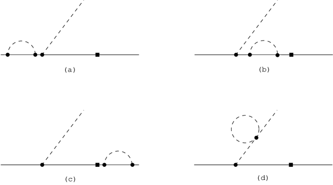
The above effective weak Hamiltonian includes only the interaction between color singlet hadron currents which is shown in Fig. 3.1(a). There is a weak interaction that four quark vertex appears in the hyperon, which is shown in Fig. 3.1(b). It corresponds to the two point vertex of the baryon operator in chiral perturbation theory. It is not enough to extract all the effects of this interaction by the factorization method from eq. (eqn:trans7). Therefore other terms have to be introduced to the effective weak Hamiltonian. These terms have the many coupling constants which are determined by the experimental data. In order to clear the hadronic currents effect of the weak Hamiltonian, we adopt the simple effective weak Hamiltonian (eqn:weak5). The effect of the two point vertex of the baryon operator in the chiral perturbation theory is discussed in ref.[23, 24]. It is also noted that the weak interaction shown in Fig. 3.1(b) do not affect the $\Delta I=3/2$ amplitudes according to the Pati and Woo theorem[21]. Hence the $\Delta I=3/2$ amplitudes are appear only in the operator $O_{4}$ and we can analyze them. In the following, we calculate the hyperon non-leptonic weak decay amplitudes with the effective Hamiltonian (eqn:weak5).

4 Hyperon Non-leptonic Weak Decays

4.1 Numerical analysis

Non-leptonic weak decay amplitude is conventionally defined by the following formula[1].

$${\cal M}(B_{i}\longrightarrow B_{f}+\pi)=G_{F}m_{{\pi}^{+}}^{2}\bar{u}_{f}(A+B\gamma_{5})u_{i},{{}}$$ (4.1)

where $A$ is the S-wave amplitude and $B$ is the P-wave one. In the heavy baryon formalism the decay amplitude is given by

$${\cal M}(B_{i}\longrightarrow B_{f}+\pi)=\frac{G_{f}}{\sqrt{2}}\bar{U}_{f}({\cal A}+(q\cdot S_{v}){\cal B})U_{i},{{}}$$ (4.2)

where $q$ is the momentum of outgoing pion. Note that $G_{F}$ and $G_{f}$ are the Fermi coupling constants but have different values: $G_{F}=10^{-5}m_{p}^{-2}$, $G_{f}=1.166\times 10^{-11}[\mbox{MeV}^{-2}]$. In the heavy baryon formalism, the baryons have the two component spinors, while baryons in eq. (eqn:ampform1) are described by four component spinors. In the rest frame of the initial baryon, the two component spinors are extracted from eq. (eqn:ampform1), and we obtain the following relations between decay amplitudes,

$$\begin{array}[]{lcl}A&=&\frac{-iG_{f}}{\sqrt{2}G_{F}m_{{\pi}^{+}}^{2}}f_{\pi}{\cal A}\\ B&=&\frac{iG_{f}}{2\sqrt{2}G_{F}m_{{\pi}^{+}}^{2}}(E_{f}+m_{f})f_{\pi}{\cal B},\end{array}{{}}$$ (4.3)

where $E_{f}$ is the energy of the final baryon and $m_{f}$ is the final state baryon mass. The hyperon non-leptonic weak decays are measured for the following seven processes:
$\Sigma^{-}\longrightarrow n+\pi^{-}\;\;\left(\Sigma^{-}_{-}\right),\;\;\;\Sigma^{+}\longrightarrow n+\pi^{+}\;\;\left(\Sigma^{+}_{+}\right),\;\;\;\Sigma^{+}\longrightarrow p+\pi^{0}\;\;\left(\Sigma^{+}_{0}\right),$
$\Lambda\longrightarrow n+\pi^{0}\;\;\left(\Lambda^{0}_{0}\right),\;\;\;\Lambda\longrightarrow p+\pi^{-}\;\;\left(\Lambda^{0}_{-}\right),\;\;\;\Xi^{-}\longrightarrow\Lambda+\pi^{-}\;\;\left(\Xi^{-}_{-}\right),\;\;\;\Xi^{0}\longrightarrow\Lambda+\pi^{0}\;\;\left(\Xi^{0}_{0}\right)$.
There are 14 measured amplitudes since each 7 decay process have the S- and P-wave amplitudes.

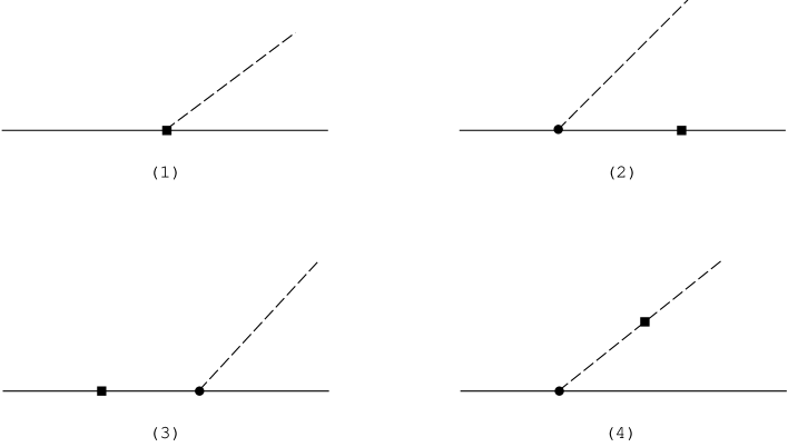
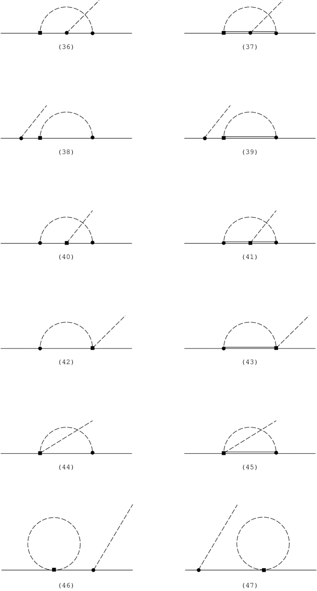
Using the strong interaction Lagrangian (eqn:mesonlag1), (eqn:mesonlag2), (eqn:baryonlag1) and the effective weak Hamiltonian (eqn:weak5), the S- and P-wave hyperon non-leptonic decay amplitudes are calculated. The tree level amplitudes are obtained from the calculation of Feynman diagrams in Fig. 4.1. Since the diagrams (2), (3) and (4) have a strong interaction vertex $(q\cdot S_{v})$, these diagrams cause only P-wave decay amplitudes. 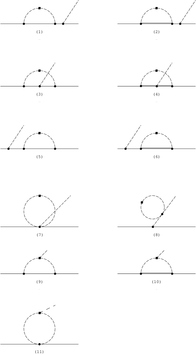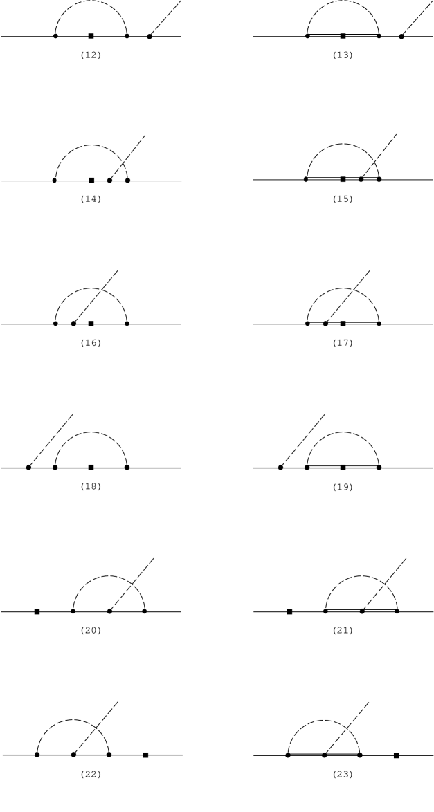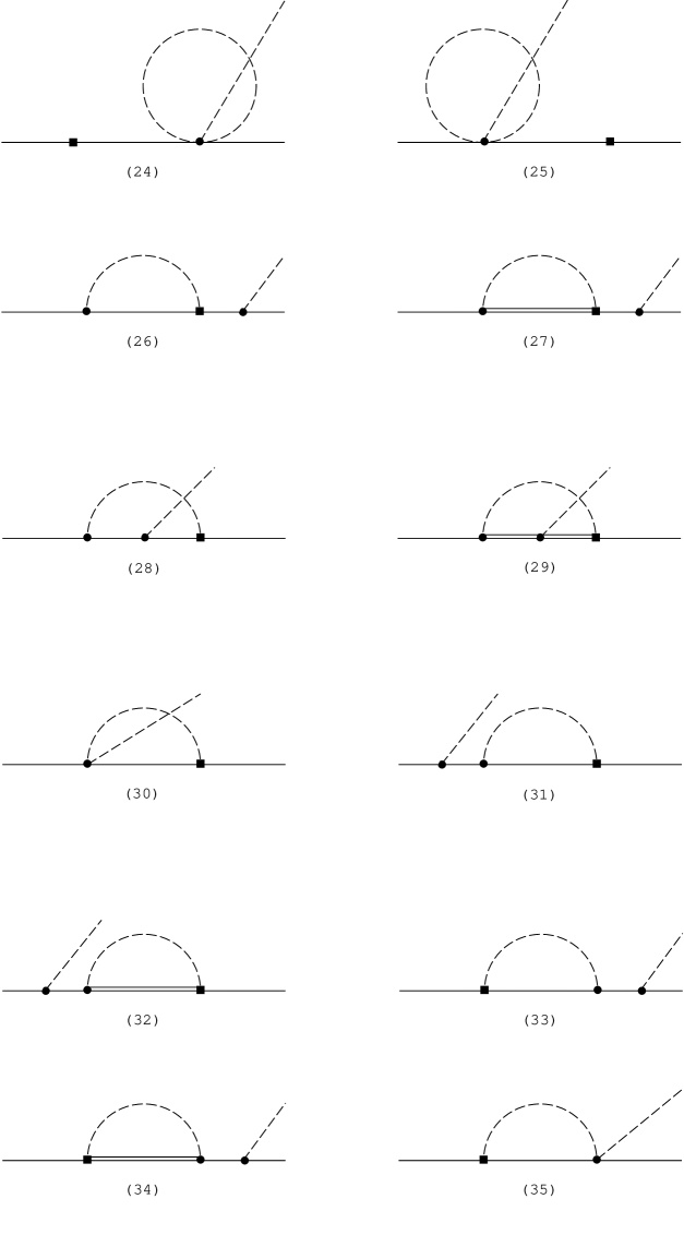The chiral logarithmic terms in the one-loop correction are obtained from the calculation of Feynman diagrams in Fig. 4.2. The S-wave amplitudes are obtained from Fig. 4.2 (9), (10), (11), (30), (35), (40), (41), (42), (43), (44), (45), (48). The rest of diagrams and (40), (41), (42), (43), (44), (45) contribute to the chiral logarithmic terms of the P-wave amplitudes. The wave function renormalization is applied to the internal and external lines of hadrons. Examples of the wave function renormalization are shown in Fig. 4.3. The amplitudes are given by the summation of these diagrams. In our study the wave function renormalization for the intermediate baryon and meson are taken into account. The tree level amplitudes are given by
S-wave:

$$\begin{array}[]{lcl}A(\Sigma^{-}_{-})&=&3.0705\times 10^{-1}-2.3337\times 10^{-1}a_{1}+2.3337\times 10^{-1}a_{2}\\ A(\Sigma^{+}_{+})&=&0\\ A(\Sigma^{+}_{0})&=&-7.0563\times 10^{-2}+1.6502\times 10^{-1}a_{1}-1.6502\times 10^{-1}a_{2}\\ A(\Lambda^{0}_{0})&=&-6.3084\times 10^{-2}-6.7368\times 10^{-2}a_{1}-2.0210\times 10^{-1}a_{2}\\ A(\Lambda^{-}_{-})&=&2.7450\times 10^{-1}+9.5273\times 10^{-2}a_{1}+2.8582\times 10^{-1}a_{2}\\ A(\Xi^{-}_{-})&=&-3.1012\times 10^{-1}+9.5273\times 10^{-2}a_{1}-2.8582\times 10^{-1}a_{2}\\ A(\Xi^{0}_{0})&=&7.1268\times 10^{-2}-6.7368\times 10^{-2}a_{1}+2.0210\times 10^{-1}a_{2}\end{array}{{}}$$ (4.4)

P-wave:

$$\begin{array}[]{lcl}B(\Sigma^{-}_{-})&=&2.2212+1.2058a_{1}+8.2856\times 10^{-1}a_{2}\\ B(\Sigma^{+}_{+})&=&-1.9490a_{1}+3.9833a_{2}\\ B(\Sigma^{+}_{0})&=&-1.2804-2.2308a_{1}+2.2308a_{2}\\ B(\Lambda^{0}_{0})&=&4.4732-1.1459\times 10^{-1}a_{1}-2.7816a_{2}\\ B(\Lambda^{0}_{-})&=&-7.7599+1.6205\times 10^{-1}a_{1}+3.9338a_{2}\\ B(\Xi^{-}_{-})&=&3.0086-1.8612a_{1}-2.7488a_{2}\\ B(\Xi^{0}_{0})&=&-1.7343+1.3161a_{1}+1.9437a_{2}\end{array}{{}}$$ (4.5)

The tree level amplitudes and the chiral logarithmic terms in the one-loop correction are given by
S-wave:

$$\begin{array}[]{lcl}A(\Sigma^{-}_{-})&=&3.2554\times 10^{1}+3.0862\times 10^{1}a_{1}-3.1032\times 10^{1}a_{2}-2.5229\times 10^{-2}c_{1}\\ A(\Sigma^{+}_{+})&=&-6.0803-1.0944\times 10^{-4}a_{1}+6.7828\times 10^{-3}a_{2}\\ A(\Sigma^{+}_{0})&=&-1.5360\times 10^{1}-2.1816\times 10^{1}a_{1}+2.1951\times 10^{1}a_{2}+1.7840\times 10^{-2}c_{1}\\ A(\Lambda^{0}_{0})&=&-3.1614\times 10^{-1}+8.8775a_{1}+2.6754\times 10^{1}a_{2}+1.0109\times 10^{-1}c_{1}\\ A(\Lambda^{0}_{-})&=&2.5155-1.2557\times 10^{1}a_{1}-3.7855\times 10^{1}a_{2}-1.4297\times 10^{-1}c_{1}\\ A(\Xi^{-}_{-})&=&-2.4018\times 10^{1}-1.2758\times 10^{1}a_{1}+3.7914\times 10^{1}a_{2}+5.3009\times 10^{-2}c_{1}\\ A(\Xi^{0}_{0})&=&1.1550\times 10^{1}+9.0225a_{1}-2.6800\times 10^{1}a_{2}-3.7483\times 10^{-2}c_{1}\end{array}{{}}$$ (4.6)

P-wave:

$$\begin{array}[]{lcl}B(\Sigma^{-}_{-})&=&6.9622\times 10^{2}+2.2896\times 10^{1}a_{1}+2.3957\times 10^{1}a_{2}+8.3649a_{3}-5.4327\times 10^{-1}c_{1}\\ B(\Sigma^{+}_{+})&=&1.4794\times 10^{2}-3.2295\times 10^{2}a_{1}+2.8974\times 10^{2}a_{2}-7.2823\times 10^{-1}c_{1}\\ B(\Sigma^{+}_{0})&=&-3.8548\times 10^{2}-2.4455\times 10^{2}a_{1}+1.8794\times 10^{2}a_{2}-5.9149a_{3}-1.3079\times 10^{-1}c_{1}\\ B(\Lambda^{0}_{0})&=&1.7307\times 10^{3}-7.6621\times 10^{1}a_{1}-3.2130\times 10^{2}a_{2}+1.6514\times 10^{1}a_{3}-5.3588\times 10^{-1}c_{1}\\ B(\Lambda^{0}_{-})&=&-2.4466\times 10^{3}+1.0836\times 10^{2}a_{1}+4.5438\times 10^{2}a_{2}-2.3354\times 10^{1}a_{3}+7.5786\times 10^{-1}c_{1}\\ B(\Xi^{-}_{-})&=&9.6124\times 10^{2}-2.9146\times 10^{2}a_{1}-3.0700\times 10^{2}a_{2}+9.9536a_{3}-3.8293\times 10^{-1}c_{1}\\ B(\Xi^{0}_{0})&=&-6.8022\times 10^{2}+2.0609\times 10^{2}a_{1}+2.1708\times 10^{2}a_{2}-7.0383a_{3}+2.7077\times 10^{-1}c_{1}\end{array}{{}}$$ (4.7)

In this computation, following hadron masses and constants are used:

$$\begin{array}[]{ccccccccc}m_{n}&=&939\mbox{[MeV]},&m_{\Sigma}&=&1193\mbox{[MeV]},&m_{\Lambda}&=&1116\mbox{[MeV]}\\ m_{\Xi}&=&1318\mbox{[MeV]},&m_{\Delta}&=&1232\mbox{[MeV]},&m_{\Sigma^{*}}&=&1385\mbox{[MeV]}\\ m_{\Xi^{*}}&=&1533\mbox{[MeV]},&m_{\Omega}&=&1672\mbox{[MeV]}&&&\\ M_{\pi}&=&138\mbox{[MeV]},&M_{K}&=&496\mbox{[MeV]},&M_{\eta}&=&547\mbox{[MeV]}\\ D&=&0.61,&F&=&0.40,&{\cal C}&=&1.6\\ {\cal H}&=&-1.9,&f_{\pi}&=&93\mbox{[Mev]},&L_{4}&=&-0.3003\\ L_{5}&=&1.399,&B_{0}&=&1391.4\mbox{[MeV]},&&&\\ \mbox{data set 2.}&&&&&&&&\\ \end{array}{{}}$$ (4.8)

And for the chiral logarithmic terms, the renormalization scale $4\pi\mu^{2}=1.0\times 10^{6}[\mbox{Mev}^{2}]$ is used. The amplitudes have 4 unknown parameters, $a_{1}$, $a_{2}$, $a_{3}$ and $c_{1}$. The constants $a_{1}$ and $a_{2}$ that appear in the scalar current are determined as $a_{1}=29.1/m_{s}$ and $a_{2}=-94.8/m_{s}$ where $m_{s}$ is the strange quark mass. They are derived from the baryon mass difference with the chiral perturbation theory[22]. The remaining two parameters are fitted with 14 experimental data. The amplitudes derived from fitted parameters are shown in Table 4.1. The fitted parameters are shown in Table 4.2. Constant terms in eq. (eqn:sloop) and (eqn:ploop) have large values, which are caused by the quark condensation value $B_{0}$. The decay amplitudes depend on the quark condensation value strongly. To reproduce the experimental data, the quark condensation value is changed as $B_{0}=1.3914\times 10^{3}\mbox{[MeV]}$, $1.3914\times 10^{2}\mbox{[MeV]}$, $0.0\mbox{[MeV]}$. Since the Table 4.1 shows that amplitudes extracted with data set 2 and $B_{0}=1.3914\times 10^{2}\mbox{[MeV]}$ have better fitting with experimental data, we adopt these parameters in the following analysis. From the Table 2.1, the difference between data set 1 and 2 are large in $K_{5}$ and $K_{6}$. This difference is responsible for the amplitudes caused by the operators $O_{5}$ and $O_{6}$. The components of the predicted amplitudes are shown in Table 4.3. The operators $O_{52}$, $O_{53}$, $O_{61}$ and $O_{62}$ which include the scalar and pseudo-scalar currents are proportional to the quark condensation value $B_{0}$. If we adopt the condition $B_{0}=0.0\mbox{[MeV]}$, The amplitudes do not depend on the parameters $a_{1}$, $a_{2}$, $a_{3}$ and $c_{1}$. The components of these amplitudes are shown in Table 4.4. These tables suggest that the contributions of the chiral logarithmic correction are large. The tree level amplitudes caused by each operator in eq. (eqn:operator3) are shown in Table 4.5 and the chiral logarithmic amplitudes caused by each operator are shown in Table 4.6.

4.2 Discussion

Table 4.1 shows that the amplitudes derived by the hadronic current interaction do not reproduce the experimental data well. It is caused by the lack of two point vertex of the baryon operator and by uncertainties of the quark condensation in scalar and pseudo-scalar currents. If we choose the condition $B_{0}=0.0\mbox{[MeV]}$, the contributions of the scalar and pseudo-scalar currents become zero. The amplitudes are, therefore, caused by the $V\pm A$ current interaction in the operator $O_{1}$, $O_{2}$, $O_{3}$, $O_{4}$ and $O_{51}$. Table 4.1 shows that the S-wave amplitudes $\Sigma^{-}_{-}$, $\Lambda^{0}_{-}$ and $\Xi^{-}_{-}$ are almost caused by the $V\pm A$ currents. In the other amplitudes the contributions of the scalar, pseudo-scalar currents and two point vertex of the baryon operator are large.

Table 4.3 and 4.4 show the large amplitudes caused by the chiral logarithmic correction. In the chiral order analysis, the logarithmic correction of the one-loop diagram has the order of magnitude, $\frac{M^{2}_{K}}{16\pi^{2}f_{\pi}^{2}}\ln\left(\frac{M^{2}_{K}}{4\pi\mu^{2}}\right)\approx 0.20$ The effect of the one-loop calculation expected to be $25\%$ correction to tree level amplitudes. But there are many loop diagrams which have many internal baryon states. Since the amplitudes are obtained by the summation of all diagrams, the amplitudes caused by the loop correction become large.

Let us considering the contribution of the each operator. In the tree level the operator $O_{1}$ is most important for the amplitudes, which is shown in Table 4.5. Since the tree level amplitudes do not depend on the free parameters $a_{3}$ and $c_{1}$, these amplitudes depend on $B_{0}$ value and they are small. The amplitudes caused by the two point vertex of the baryon operator must be large. But in the chiral logarithmic correction, the operators composed of the scalar and pseudo-scalar currents become important. Especially the weak Hamiltonian caused by meson currents, which is shown in Fig.fig:loop (9), (10) etc., is important since these terms are proportional to $B^{2}_{0}$ and sensitive to the $B_{0}$ value. In order to reproduce the experimental data by the chiral perturbation theory, it is important to construct the $O_{5}$ and $O_{6}$ operators exactly.

In our method $\Delta I=3/2$ amplitudes are derived from the operator $O_{4}$ and it does not depend on the unknown coupling constant in the chiral perturbation theory. In the tree level, the S-wave $\Delta I=3/2$ amplitudes are given by the diagram (1) in Fig.fig:tree and the P-wave amplitudes are given by the diagrams (1) and (4) in Fig.fig:tree. The chiral logarithmic corrections of the S-wave $\Delta I=3/2$ amplitudes are obtained from the diagrams (9), (10), (11), (30), (35), (40), (41) and (48) in Fig.fig:loop, and the P-wave amplitudes are obtained from the diagrams (1)$\sim$(8), (26)$\sim$(29), (31)$\sim$(34), (36)$\sim$(41) and (48) in Fig.fig:loop. The comparison between the experimental data and the calculated data with our method are shown in Table 4.7. In the tree level, the absolute values of the $\Delta I=3/2$ amplitudes become small. It is consistent to the $\Delta I=1/2$ rule. These small amplitudes are caused by the small coupling constants $F,\;D<1$ in the chiral perturbation theory. But including the chiral logarithmic correction of the one-loop diagrams, the amplitudes become large. These amplitudes are caused by the summation of the many logarithmic term in loop diagrams and by the large coupling constants $|{\cal H}|,\;{\cal C}>1$ of the decuplet fields.

5 Conclusion

Hyperon non-leptonic weak decay amplitudes are studied by the chiral perturbation theory. Applying the renormalization method to the weak interaction, the effective weak Hamiltonian which has perturbative QCD correction is obtained. The effective weak Hamiltonian is described by the qurak bilinear form. These quark currents are substituted by the hadronic currents derived by the chiral perturbation theory.

Our results suggest that the color singlet $V\pm A$ current interaction has the small contribution to the decay amplitudes. The weak interaction caused by the scalar, pseudo-scalar currents and by the two point vertex of the baryon operator have the large contribution. The $\Delta I=3/2$ amplitudes are suppressed. Using the chiral perturbation theory as the strong interaction correction for the weak interaction, it is consistent to the experimental data. Our method have no parameters for the $\Delta I=3/2$ amplitudes. Applying our method to the more complicated decay process, like $Y+N\longrightarrow N+N$, it is possible to predict the characteristic of the $\Delta I=3/2$ amplitudes.

In order to reproduce the experimental data quite well, it is necessary to study the two point vertex of the baryon operator, the quark condensation value $B_{0}$ for the weak interaction and the relation between the renormalization scale $\mu$ of the perturbative QCD correction and the chiral perturbation theory.

Table 2.1     The values of the coefficients in the effective weak Hamiltonian (eqn:weak4). The values are taken from Ref. [11]. The data set 1 corresponds to the choices $m_{t}=200$[GeV] and $\mu_{0}=0.24$[GeV], $\Lambda_{QCD}=0.10$. The data set 2 corresponds to the choices $m_{t}=200$[GeV] and $\mu_{0}=0.71$[GeV], $\Lambda_{QCD}=0.316$. In both cases, $\mu_{0}$ is defined so as to satisfy $\alpha_{s}(\mu^{2})=1$.

	data set 1	data set 2
$\mu$(GeV)	0.24	0.71
$\Lambda^{(4)}$(GeV)	0.10	0.316
$K_{1}$	-0.284	-0.270
$K_{2}$	0.009	0.011
$K_{3}$	0.026	0.027
$K_{4}$	0.026	0.027
$K_{5}$	0.004	0.002
$K_{6}$	0.004	0.002

Table 3.1     Phenomenological values of the renormalized couplings $L_{i}^{r}(M_{\rho})$. $L^{r}_{i}(i=4,\cdots,8)$ are from ref. [15], $L^{r}_{9,10}$ from ref. [19] and $L^{r}_{1,2,3}$ from ref. [20].

i	$L_{i}^{r}(M_{\rho})$
1	0.7$\pm$0.5
2	1.2$\pm$0.4
3	-3.6$\pm$1.3
4	-0.3$\pm$0.5
5	1.4$\pm$0.5
6	-0.2$\pm$0.3
7	-0.4$\pm$0.15
8	0.9$\pm$0.3
9	6.9$\pm$0.2
10	-5.2$\pm$0.3

Table 4.1     The tree and one-loop level amplitudes. First column corresponds to the experimental data. The quark condensation value $B_{0}$ is varied as $B_{0}=1.3914\times 10^{3}\mbox{[MeV]}$, $B_{0}=1.3914\times 10^{2}\mbox{[MeV]}$ and $B_{0}=0.0\mbox{[MeV]}$.

S-wave:
decay		data set 1			data set 2
mode	exp.	$1.3941\times 10^{3}$	$1.3941\times 10^{2}$	$0.0$	$1.3941\times 10^{3}$	$1.3941\times 10^{2}$	$0.0$
$\Sigma^{-}_{-}$	$1.93\pm 0.01$	93.06	6.157	1.732	45.32	4.016	1.717
$\Sigma^{+}_{+}$	$0.06\pm 0.01$	-12.75	-0.1616	-0.03402	-6.082	-0.09894	-0.03831
$\Sigma^{+}_{0}$	$-1.48\pm 0.05$	-50.80	-3.278	-0.2901	-24.39	-1.805	-0.2463
$\Lambda^{0}_{0}$	$-1.07\pm 0.02$	-14.24	-6.484	-0.5509	-7.790	-4.1018	-0.4985
$\Lambda^{0}_{-}$	$1.47\pm 0.01$	23.13	10.35	1.938	13.09	7.012	1.907
$\Xi^{-}_{-}$	$-2.04\pm 0.01$	-75.01	-7.689	-2.173	-37.17	-5.175	-2.142
$\Xi^{0}_{0}$	$1.54\pm 0.03$	42.63	4.480	0.6749	20.85	2.719	0.6203

P-wave:
decay		data set 1			data set 2
mode	exp.	$1.3941\times 10^{3}$	$1.3941\times 10^{2}$	$0.0$	$1.3941\times 10^{3}$	$1.3941\times 10^{2}$	$0.0$
$\Sigma^{-}_{-}$	$-0.65\pm 0.07$	-433.8	-3.070	2.304	-204.2	0.5967	2.316
$\Sigma^{+}_{+}$	$19.07\pm 0.07$	31.33	15.84	7.479	24.19	16.83	7.216
$\Sigma^{+}_{0}$	$12.04\pm 0.58$	330.8	15.75	6.038	163.7	13.95	5.935
$\Lambda^{0}_{0}$	$-7.14\pm 0.56$	128.9	-4.52	-0.5050	58.51	-4.901	-0.4810
$\Lambda^{0}_{-}$	$9.98\pm 0.24$	-179.9	6.079	0.3647	-81.83	6.581	0.3174
$\Xi^{-}_{-}$	$6.93\pm 0.31$	-71.30	1.399	0.4604	-34.72	-0.1677	0.4341
$\Xi^{0}_{0}$	$-6.43\pm 0.66$	49.51	-1.167	-0.4958	24.02	-0.06164	-0.4837

Table 4.2     The parameters of scalar and pseudo-scalar currents. Two types of data set are used. Fixing the $B_{0}$ value, we obtain eq. (eqn:stree), (eqn:ptree), (eqn:sloop) and (eqn:ploop). The parameters are fitted with least square method.

parameter	dataset 1
$B_{0}$	$1.3914\times 10^{3}$	$1.3914\times 10^{2}$	0.0
$a_{1}$	$1.9400\times 10^{-1}$	$1.9400\times 10^{-1}$	-
$a_{2}$	$-6.3200\times 10^{-1}$	$-6.3200\times 10^{-1}$	-
$a_{3}$	$-1.0652\times 10^{2}$	$-2.3960\times 10^{1}$	-
$c_{1}$	$8.9337$	$-2.0402\times 10^{2}$	-

parameter	dataset 2
$B_{0}$	$1.3914\times 10^{3}$	$1.3914\times 10^{2}$	0.0
$a_{1}$	$1.9400\times 10^{-1}$	$1.9400\times 10^{-1}$	-
$a_{2}$	$-6.3200\times 10^{-1}$	$-6.3200\times 10^{-1}$	-
$a_{3}$	$-1.0692\times 10^{2}$	$-2.7993\times 10^{1}$	-
$c_{1}$	$1.1855$	$-2.8150\times 10^{2}$	-

Table 4.3    The predicted amplitudes with $B_{0}=1.3941\times 10^{2}\mbox{[MeV]}$, data set 2 and the parameters in Table 4.2. $A_{exp}$ and $B_{exp}$ correspond to the experimental data. $A_{tree}$ and $B_{tree}$ are the tree level amplitudes. $\Delta A_{loop}$ and $\Delta B_{loop}$ are the summation of the chiral logarithmic correction of the one-loop graphs. They are represented with $\Delta A_{loop}=\Delta A_{octet}+\Delta A_{decuplet}$ and $\Delta B_{loop}=\Delta B_{octet}+\Delta B_{decuplet}$. $A_{theory}$ and $B_{theory}$ are the total amplitude of the chiral perturbation theory, which are represented with $A_{theory}=A_{tree}+\Delta A_{loop}$ and $B_{theory}=B_{tree}+\Delta B_{loop}$.

S-wave:
decay mode	$A_{exp.}$	$A_{theory}$	$A_{tree}$	$\Delta A_{loop}$	$\Delta A_{octet}$	$\Delta A_{decuplet}$
$\Sigma_{-}^{-}$	$1.93\pm 0.01$	4.016	0.2974	3.719	1.739	1.980
$\Sigma_{+}^{+}$	$0.06\pm 0.01$	-0.09894	0.0	-0.09894	-0.04420	-0.05474
$\Sigma^{+}_{0}$	$-1.48\pm 0.05$	-1.805	-0.06375	-1.741	-1.149	-0.5920
$\Lambda_{0}^{0}$	$-1.07\pm 0.02$	-4.102	-0.05735	-4.044	-0.6702	-3.374
$\Lambda^{0}_{-}$	$1.47\pm 0.01$	7.012	0.2664	6.746	1.619	5.127
$\Xi^{-}_{-}$	$-2.04\pm 0.01$	-5.175	-0.3002	-4.875	-1.880	-2.995
$\Xi^{-}_{0}$	$1.54\pm 0.03$	2.719	0.06423	2.655	1.109	1.546

P-wave:
decay mode	$B_{exp.}$	$B_{theory}$	$B_{tree}$	$\Delta B_{loop}$	$\Delta B_{octet}$	$\Delta B_{decuplet}$
$\Sigma_{-}^{-}$	$-0.65\pm 0.07$	0.5967	0.6097	-0.01300	-17.31	17.29
$\Sigma_{+}^{+}$	$19.07\pm 0.07$	16.83	-0.1448	16.98	-11.31	28.29
$\Sigma^{+}_{0}$	$12.04\pm 0.58$	13.95	-0.2433	14.19	4.578	9.615
$\Lambda_{0}^{0}$	$-7.14\pm 0.56$	-4.901	0.6148	-5.516	-19.30	13.79
$\Lambda^{0}_{-}$	$9.98\pm 0.24$	6.581	-2.303	8.885	26.22	-17.34
$\Xi^{-}_{-}$	$6.93\pm 0.31$	-0.1677	0.9142	-1.081	-10.93	9.851
$\Xi^{-}_{0}$	$-6.43\pm 0.66$	-0.06164	-0.2534	0.1917	8.392	-8.200

Table 4.4    The predicted amplitudes with $B_{0}=0.0\mbox{[MeV]}$, data set 2. $A_{exp}$ and $B_{exp}$ correspond to the experimental data. $A_{tree}$ and $B_{tree}$ are the tree level amplitudes. $\Delta A_{loop}$ and $\Delta B_{loop}$ are the summation of the chiral logarithmic correction of the one-loop graphs. They are represented with $\Delta A_{loop}=\Delta A_{octet}+\Delta A_{decuplet}$ and $\Delta B_{loop}=\Delta B_{octet}+\Delta B_{decuplet}$. $A_{theory}$ and $B_{theory}$ are the total amplitude of the chiral perturbation theory, which are represented with $A_{theory}=A_{tree}+\Delta A_{loop}$ and $B_{theory}=B_{tree}+\Delta B_{loop}$.

S-wave:
decay mode	$A_{exp.}$	$A_{theory}$	$A_{tree}$	$\Delta A_{loop}$	$\Delta A_{octet}$	$\Delta A_{decuplet}$
$\Sigma_{-}^{-}$	$1.93\pm 0.01$	1.717	0.3071	1.410	0.3558	1.054
$\Sigma_{+}^{+}$	$0.06\pm 0.01$	-0.03831	0.0	-0.03831	-0.04977	0.01146
$\Sigma^{+}_{0}$	$-1.48\pm 0.05$	-0.2463	-0.07056	-0.1757	-0.2162	0.04050
$\Lambda_{0}^{0}$	$-1.07\pm 0.02$	-0.4985	-0.06308	-0.4354	0.07263	-0.5080
$\Lambda^{0}_{-}$	$1.47\pm 0.01$	1.907	0.2745	1.633	0.5580	1.075
$\Xi^{-}_{-}$	$-2.04\pm 0.01$	-2.142	-0.3101	-1.832	-0.4793	-1.353
$\Xi^{-}_{0}$	$1.54\pm 0.03$	0.6203	0.07127	0.5490	0.1440	0.4050

P-wave:
decay mode	$B_{exp.}$	$B_{theory}$	$B_{tree}$	$\Delta B_{loop}$	$\Delta B_{octet}$	$\Delta B_{decuplet}$
$\Sigma_{-}^{-}$	$-0.65\pm 0.07$	2.316	0.6080	1.708	-0.6232	2.331
$\Sigma_{+}^{+}$	$19.07\pm 0.07$	7.216	0.0	7.216	-0.02100	7.237
$\Sigma^{+}_{0}$	$12.04\pm 0.58$	5.935	-0.1397	6.075	0.7635	5.312
$\Lambda_{0}^{0}$	$-7.14\pm 0.56$	-0.4810	0.4882	-0.9692	0.06545	-1.035
$\Lambda^{0}_{-}$	$9.98\pm 0.24$	0.3174	-2.124	2.442	-1.179	3.621
$\Xi^{-}_{-}$	$6.93\pm 0.31$	0.4341	0.8236	-0.3894	0.6008	-0.9902
$\Xi^{-}_{0}$	$-6.43\pm 0.66$	-0.4837	-0.1893	-0.2945	0.2395	-0.5340

Table 4.5    The amplitudes for each operator in the tree level calculation with data set 2 and $B_{0}=1.3914\times 10^{2}\mbox{[MeV]}$. The first column corresponds to the operator number of the effective Hamiltonian (eqn:weak5) and (eqn:operator3). The second row shows the observed data.

S-wave:
vertex	$\Sigma_{-}^{-}$	$\Sigma_{+}^{+}$	$\Sigma^{+}_{0}$	$\Lambda_{0}^{0}$	$\Lambda^{0}_{-}$	$\Xi^{-}_{-}$	$\Xi^{-}_{0}$
exp.	1.93	0.06	-1.48	-1.07	1.47	-2.04	-1.54
$O_{1}$	0.2073	0	-0.1466	-0.1310	0.1853	-0.2093	0.1480
$O_{2}$	0.01689	0	-0.01194	-0.01068	0.01510	-0.01706	0.01206
$O_{3}$	0.01382	0	-0.009770	-0.008735	0.01235	-0.01396	0.009868
$O_{4}$	0.06909	0	0.09770	0.08735	0.06176	-0.06978	-0.09868
$O_{51}$	0	0	0	0	0	0	0
$O_{52}$	3.755E-4	0	-2.655E-4	-2.234E-4	3.159E-4	-3.879E-4	2.743E-4
$O_{53}$	0	0	0	0	0	0	0
$O_{61}$	-0.01001	0	0.007081	0.005956	-0.008424	0.01034	-0.007314
$O_{62}$	0	0	0	0	0	0	0

P-wave:
vertex	$\Sigma_{-}^{-}$	$\Sigma_{+}^{+}$	$\Sigma^{+}_{0}$	$\Lambda_{0}^{0}$	$\Lambda^{0}_{-}$	$\Xi^{-}_{-}$	$\Xi^{-}_{0}$
exp.	-0.65	19.07	12.04	-7.14	9.98	6.93	-6.43
$O_{1}$	0.4104	0	-0.2902	1.01387	-1.434	0.5559	-0.3931
$O_{2}$	0.03344	0	-0.02365	0.08261	-0.1168	0.04530	-0.03203
$O_{3}$	0.02736	0	-0.01935	0.06759	-0.09559	0.03706	-0.02621
$O_{4}$	0.1368	0	0.1935	-0.6759	-0.4779	0.1853	0.2621
$O_{51}$	0	0	0	0	0	0	0
$O_{52}$	6.199E-4	0.005641	0.003550	-0.003244	0.004588	-0.002606	0.001842
$O_{53}$	-6.840E-4	0	4.837E-4	-0.001690	0.002390	-9.265E-4	6.551E-4
$O_{61}$	-0.01653	-0.1504	-0.09467	0.08651	-0.1223	0.06948	-0.04913
$O_{62}$	0.01824	0	-0.01290	0.04506	-0.06373	0.02471	-0.01747

Table 4.6    The amplitudes for each operator, which are derived from the one-loop calculation with data set 2 and $B_{0}=1.3914\times 10^{2}\mbox{[MeV]}$. The first column corresponds to the operator number of the effective Hamiltonian (eqn:weak5) and (eqn:operator3). The second row shows the observed data.

S-wave:
vertex	$\Sigma_{-}^{-}$	$\Sigma_{+}^{+}$	$\Sigma^{+}_{0}$	$\Lambda_{0}^{0}$	$\Lambda^{0}_{-}$	$\Xi^{-}_{-}$	$\Xi^{-}_{0}$
exp.	1.93	0.06	-1.48	-1.07	1.47	-2.04	-1.54
$O_{1}$	0.8109	0.03720	-0.5395	-0.7886	1.124	-1.212	0.8587
$O_{2}$	0.06608	0.003031	-0.04396	-0.06425	0.09157	-0.09876	0.06996
$O_{3}$	0.1346	0.004306	-0.09025	-0.06023	0.08568	-0.1685	0.1178
$O_{4}$	0.3988	-0.08284	0.4980	0.4776	0.3318	-0.3530	-0.4974
$O_{51}$	0	0	0	0	0	0	0
$O_{52}$	-0.02663	0	0.01884	0.1102	-0.1558	0.05705	-0.04033
$O_{53}$	-0.06330	0.002354	0.04215	0.03044	-0.04338	0.06150	-0.04172
$O_{61}$	0.7101	-0.0002238	-0.5023	-2.938	4.156	-1.521	1.075
$O_{62}$	1.688	-0.06277	-1.124	-0.8116	1.157	-1.640	1.113

P-wave:
vertex	$\Sigma_{-}^{-}$	$\Sigma_{+}^{+}$	$\Sigma^{+}_{0}$	$\Lambda_{0}^{0}$	$\Lambda^{0}_{-}$	$\Xi^{-}_{-}$	$\Xi^{-}_{0}$
exp.	-0.65	19.07	12.04	-7.14	9.98	6.93	-6.43
$O_{1}$	0.5634	6.890	4.473	-1.549	2.191	0.007857	-0.005556
$O_{2}$	0.05174	0.5680	0.3650	-0.1240	0.1753	0.005649	-0.003995
$O_{3}$	0.06527	-0.2370	-0.2137	0.1996	-0.2822	-0.1340	0.09473
$O_{4}$	1.028	-0.004212	1.450	0.5049	0.3570	-0.2686	-0.3799
$O_{51}$	-3.976E-4	-4.487E-4	-3.612E-5	-1.561E-4	2.207E-4	-3.415E-4	2.415E-4
$O_{52}$	-0.8817	-0.7550	0.08955	-1.337	1.892	-0.8356	0.5909
$O_{53}$	0.9487	0.3746	-0.4058	1.515	-2.143	0.8626	-0.6098
$O_{61}$	23.51	20.13	-2.388	35.67	-50.44	22.28	-15.76
$O_{62}$	-25.30	-9.990	10.82	-40.39	57.13	-23.00	16.26

Table 4.7    The S- and P-wave $\Delta I=3/2$ amplitudes of each decay mode. The second column shows the experimentally obtained ratio of $\Delta I=3/2$ and $\Delta I=1/2$ amplitudes. The third column represents the $\Delta I=3/2$ amplitudes which are calculated with the total decay amplitude and the ratio of the second column. The fourth and fifth column show the $\Delta I=3/2$ amplitude obtained by the effective weak Hamiltonian (eqn:weak5).

S-wave
decay mode	$A^{3/2}/A^{1/2}$	$A^{3/2}_{exp.}$	$A^{3/2}_{tree}$	$A^{3/2}_{tree+loop}$
$\Sigma^{-}_{-}$	$-0.061\pm 0.024$	-0.1254	0.06909	0.4679
$\Sigma^{+}_{+}$	$-0.061\pm 0.024$	-0.003898	0.0	-0.08284
$\Sigma^{+}_{0}$	$-0.061\pm 0.024$	0.09614	0.09770	0.5957
$\Lambda^{0}_{0}$	$0.027\pm 0.008$	-0.02813	0.08735	0.5650
$\Lambda^{0}_{-}$	$0.027\pm 0.008$	0.03865	0.06176	0.3936
$\Xi^{-}_{-}$	$-0.038\pm 0.014$	0.08058	-0.06978	-0.4228
$\Xi^{0}_{0}$	$-0.038\pm 0.014$	-0.06083	-0.09868	-0.5961

P-wave
decay mode	$B^{3/2}/B^{1/2}$	$B^{3/2}_{exp.}$	$B^{3/2}_{tree}$	$B^{3/2}_{tree+loop}$
$\Sigma^{-}_{-}$	$-0.074\pm 0.027$	0.05194	0.1368	1.165
$\Sigma^{+}_{+}$	$-0.074\pm 0.027$	-1.524	0.0	-0.004212
$\Sigma^{+}_{0}$	$-0.074\pm 0.027$	-0.9622	0.1935	1.644
$\Lambda^{0}_{0}$	$0.030\pm 0.037$	-0.2080	-0.6759	-0.1710
$\Lambda^{0}_{-}$	$0.030\pm 0.037$	0.2907	-0.4779	-0.1209
$\Xi^{-}_{-}$	$-0.17\pm 0.09$	-1.419	0.1853	-0.0833
$\Xi^{0}_{0}$	$-0.17\pm 0.09$	1.317	0.2621	-0.1178

Figure 3.1: $\Delta S=1$ hyperon non-leptonic weak decay of quark currents. (a) corresponds to the weak interaction between two hadronic currents which are color singlet. (b) corresponds to the weak interaction inside the hyperon.

Figure 4.1: Tree graph for hyperon non-leptonic decay. Single solid lines represent octet baryon fields and dots lines represent meson fields. The solid square denotes $\Delta S=1$ weak interaction vertices and the solid dot denotes strong interaction vertices.

Figure 4.2: One loop diagrams for hyperon non-leptonic weak decay. Single solid lines represent octet baryon fields, double solid lines represents decuplet fields and dots lines denote meson fields. the solid square denotes $\Delta S=1$ weak interaction vertices and the solid dot denotes strong interaction vertices.

Figure 4.2: (continued)

Figure 4.2: (continued)

Figure 4.2: (continued)

Figure 4.2: (continued)

Figure 4.3: Examples of the wave function renormalization applied to the tree diagram in Figure 4.2 (2). In this study, it is considered that the internal baryon state is the decuplet baryon.

References

• [1] Review of Particle Properties, Phys. Lett.  B111 (1982) 286
• [2] J. Bijnens, H. Sonoda and M. B. Wise, Nucl. Phys.  B261 (1985) 185
• [3] J. F. Donoghue, E. Golowich and B. Holstein, Phys. Rep. 131 (1986) 319
• [4] E. Jenkins, Nucl. Phys.  B375 (1992) 561
• [5] R. Springer, preprint DUKE-95-95
• [6] B. Borasoy and B. R. Holstein ,”Non-leptonic Hyperon Decays in Chiral Perturbation Theory” hep-ph/9805430
• [7] S. Weinberg, Phys. Rev. Lett.  19 (1967) 1264,
A. Salam : in Elementary Particle Theory ed. by N. Svartholom
• [8] D. Bailin, “Weak Interaction”, (Adam Hilger LTD, Bristol, 1982)
• [9] A. I. Valnshtein, V. I. Zakharov and M. A. Shifman JETP 45 (’77) 670
• [10] F. J. Gilman and M. B. Wise, Phys. Rev.  D20 (1979) 2392
• [11] E. A. Paschos, T. Schneider and Y. L. Wu, Nucl. Phys.  B332 (1990) 285
• [12] L. B. Okun, Leptons and Quarks (North-Holland, Netherland, 1982)
• [13] M. Kobayashi and T. Maskawa, Prog. Theor. Phys. 49 (1973) 652
• [14] W. A. Bardeen, A. J. Buras and J.-M. Gerard, Phys. Lett.  B192 (1987) 138
W. A. Bardeen, A. J. Buras and J.-M. Gerard, Nucl. Phys.  B293 (1987) 787
• [15] J. Gasser and H. Leutwyler Ann. Phys. (N.Y.) 158 (1984) 142; Nucl. Phys.  B250 (1985) 465; Nucl. Phys.  B250 (1985) 517; Nucl. Phys.  B250 (1985) 539
• [16] S. Weinberg, Physica 96A (1979) 327
• [17] E. Jenkins and A. V. Manohar, Phys. Lett.  B255 (1991) 558
• [18] E. Jenkins and A. V. Manohar, Phys. Lett.  B259 (1991) 353
• [19] J. Bijnens and F. Cornet, Nucl. Phys.  B296 (1988) 557
• [20] J. Bijnens, G. Ecker and J. Gasser, in :The DAFNE Physics Handbook (vol. 1),
eds. L. Maiani, G. Pancheri and N. Paver, INFN Frascati, 1992
• [21] J. C. Pati and C. H. Woo, Phys. Rev.  D3 (1971) 2920
• [22] E. Jenkins, Nucl. Phys.  B368 (1992) 190
• [23] K. Takayama, Thesis, Tokyo Institute of Technology 1997
• [24] in preparation