Quasi-real photon production
in thermal QCD

Abstract

In this proceedings, I consider two-loop contributions to real photon production in thermal QCD. If the photon is strictly massless, strong collinear divergences appear in this calculation. These singularities are regularized by the quark thermal mass of order $gT$, which generates powers of $1/g$, so that the corresponding terms are strongly enhanced with respect to naive expectations of their order of magnitude.

LAPTH-98/699, hep-ph/9809380

I Introduction

From a phenomenological point of view, photon production is considered as a potential candidate for the detection and discrimination of a quark gluon plasma. This quantity is also interesting from a more formal point of view in order to test our control over some aspects of thermal field theories like infrared and collinear singularities. One reason is that this quantity is obviously observable and should therefore be infrared and collinear safe in a consistent theory.

At one loop, the thermal production of soft real photons [1, 2] suffers from a logarithmic collinear singularity, that can be cured by an extension of the hard thermal loop resummation technique proposed by Flechsig and Rebhan [3]. It appeared also that common processes like bremsstrahlung are not present at one loop, while they are assumed to play the dominant role in semi-classical approaches [4, 5, 6, 7].

Therefore, we considered the two-loop diagrams giving bremsstrahlung [8, 9, 10]. It turns out that they suffer from collinear singularities much stronger than the 1-loop ones. After regularization by a thermal mass of order $gT$, these singularities give extra factors $1/g$, which spoils the natural hierarchy of perturbative expansion. I present this calculation in this proceedings. Then, I compare the result with that of other approaches, and finally, I conclude with some open questions related to what might happen at higher orders.

II Tools

A Hard thermal loops

This first section is devoted to a presentation of the tools we used in order to perform this calculation. The general framework of our study is the effective perturbative expansion that one obtains after the resummation of hard thermal loops [11, 12]. To be more definite, we used the retarded-advanced version of the real time formalism [13, 14]. Initially, one of the motivations for hard thermal loops was the resolution of the long standing puzzle of the gluon damping rate, but they provided also a consistent framework to deal with the infrared sector of thermal theories.

B Counterterms

A possible way to implement calculations in this effective theory is to use cut-offs [15]: loops with effective propagators and vertices are evaluated with an upper cut-off $\Lambda$ ($gT\ll\Lambda\ll T$). If higher order corrections are not necessary, the cut-off dependence is usually of a smaller order of magnitude. If on the contrary an important dependence on $\Lambda$ is observed, then one must include higher order diagrams correcting this loop, in which $\Lambda$ must be used as a lower cut-off to prevent double counting.

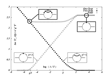
FIG. 1.: Cancellation of cut-off dependence illustrated on the example of Baier et al. This figure also shows the 1-loop and 2-loop contributions when one does not use a cut-off (diagrams in boldface boxes).

One should then check that the sum of both terms is $\Lambda$ independent at the desired order. This procedure has been used also in [16] to calculate the hard real photon production rate. The results are illustrated graphically on figure 1, which represents numerical evaluations of one- and two-loop contributions to the photon polarization tensor.

This procedure can also be interpreted more formally in terms of an effective lagrangian and counterterms. The proper way to perform the hard thermal loop resummation is to write an effective lagrangian ${\cal L}_{\rm eff}$ which is the sum of the bare lagrangian $\cal L$ and of the term ${\cal L}_{{}_{\rm HTL}}$ containing all the hard thermal corrections [17, 18]. Therefore, it appears clearly that one needs to subtract counterterms in order to keep the overall lagrangian unmodified. Basically, this procedure amounts to write

$${\cal L}={\cal L}_{\rm eff}+{\cal L}_{\rm ct}$$ (1)

$${\cal L}_{\rm eff}={\cal L}+{\cal L}_{{}_{\rm HTL}}$$ (2)

$${\cal L}_{\rm ct}=-{\cal L}_{{}_{\rm HTL}}\;.$$ (3)

That way, the HTL resummation is just a mere reordering of the perturbative expansion, and the exact theory remains the same. Counterterms have been used in [19] for the two-loop plasmon mass.

The subtraction of counterterms and the use of cut-offs are equivalent. This is illustrated on figure 1, where we also represented the 1-loop and 2-loop contributions when the cut-off is removed, in the boldface boxes. Obviously, their sum is much higher than the value of the plateau in the cut-off approach. This means that this sum includes some contributions twice, and that a counterterm is mandatory.

Counterterms seem more systematic since they come from a lagrangian formulation, while it can be tricky to use properly cut-offs in a situation with overlapping loops. In the following, I follow the point of view based on counterterms.

C Photon production rate

Let me now give the precise relationship between the photon production rate and the thermal Green’s functions. The number of real photons emitted per unit time and per unit volume of the plasma is related to the retarded photon self energy via [20, 21]

$${{dN}\over{dtd^{3}\mathchoice{{\hbox{\boldmath$\displaystyle x$}}}{{\hbox{\boldmath$\textstyle x$}}}{{\hbox{\boldmath$\scriptstyle x$}}}{{\hbox{\boldmath$\scriptscriptstyle x$}}}}}=-{{d^{3}\mathchoice{{\hbox{\boldmath$\displaystyle q$}}}{{\hbox{\boldmath$\textstyle q$}}}{{\hbox{\boldmath$\scriptstyle q$}}}{{\hbox{\boldmath$\scriptscriptstyle q$}}}}\over{(2\pi)^{3}2q_{o}}}2n_{{}_{B}}(q_{o}){\rm Im}\,\Pi^{{}^{RA}}{}_{\mu}{}^{\mu}(q_{o},\mathchoice{{\hbox{\boldmath$\displaystyle q$}}}{{\hbox{\boldmath$\textstyle q$}}}{{\hbox{\boldmath$\scriptstyle q$}}}{{\hbox{\boldmath$\scriptscriptstyle q$}}})\;,$$ (4)

where $n_{{}_{B}}(q_{o})\equiv 1/(\exp(q_{o}/T)-1)$ is the Bose-Einstein statistical factor. For photons of invariant mass $Q^{2}>0$ subsequently decaying in a lepton pair, we have instead

$${{dN}\over{dtd^{3}\mathchoice{{\hbox{\boldmath$\displaystyle x$}}}{{\hbox{\boldmath$\textstyle x$}}}{{\hbox{\boldmath$\scriptstyle x$}}}{{\hbox{\boldmath$\scriptscriptstyle x$}}}}}=-{{dq_{o}d^{3}\mathchoice{{\hbox{\boldmath$\displaystyle q$}}}{{\hbox{\boldmath$\textstyle q$}}}{{\hbox{\boldmath$\scriptstyle q$}}}{{\hbox{\boldmath$\scriptscriptstyle q$}}}}\over{12\pi^{4}}}{\alpha\over{Q^{2}}}\,n_{{}_{B}}(q_{o}){\rm Im}\,\Pi^{{}^{RA}}{}_{\mu}{}^{\mu}(q_{o},\mathchoice{{\hbox{\boldmath$\displaystyle q$}}}{{\hbox{\boldmath$\textstyle q$}}}{{\hbox{\boldmath$\scriptstyle q$}}}{{\hbox{\boldmath$\scriptscriptstyle q$}}})\;.$$ (5)

Basically, the second formula differs from the first one by the allowed phase space, by the propagator $1/Q^{2}$ of a massive photon, and by the coupling constant $\alpha$ which appears in the decay into a lepton pair. The imaginary part of the retarded self energy appearing in the right hand side can be expressed as a sum of cuts through the corresponding diagrams [22, 23, 24].

III Two-loop contributions

A Involved topologies

Bremsstrahlung appears in the two-loop diagrams represented on figure 2.

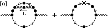
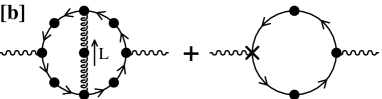
FIG. 2.: Two-loop contributions involving bremsstrahlung processes. A black dot denotes an effective propagator or vertex. Crosses are HTL counterterms.

According to the discussion made earlier, they should be accompanied by the 1-loop diagrams involving the proper HTL counterterms. In fact, these two-loop diagrams contain much more than bremsstrahlung. For instance, if we consider a cut that goes through the gluon propagator, we can have bremsstrahlung if the gluon is space-like ($L^{2}<0$) and corrections to Compton effect if $L^{2}>0$. Concerning the counterterms, since their role is to avoid double counting, it is quite natural to associate them with the contributions coming from the $L^{2}>0$ region of phase space. Indeed, the inner structure of the counterterm involves a bare gluon which contributes only in the time-like region once cut. Another way to justify this is to say that the counterterms should be associated with terms that provide corrections to a process appearing already at a lower order. There is no point in associating counterterms with a process that appears in this order for the first time. Therefore, counterterms will be calculated only if it appears that the $L^{2}>0$ region contributes at leading order.

Phase space considerations tend to make us favor a hard quark loop in order to enlarge its size as much as possible. Therefore, we can drop at leading order hard thermal corrections involving the propagator of such a hard quark, and obtain a simplified version of the previous diagrams, which is represented on figure 3.

FIG. 3.: Simplified two-loop contributions. The circled vertices correspond to the framework of the cutting rules.

More precisely, we will use the hard limit of the effective quark propagator, retaining that way an asymptotic thermal mass. This mass will be necessary later in order to regularize collinear singularities. Other authors [25, 26] have found that the width obtained by an extra resummation including a self energy with an imaginary part in the time like region may compete with this asymptotic mass as a collinear regulator under certain circumstances. But since our goal was to follow strictly the HTL approach, we did not consider this extension here.

B Matrix element

We have checked that the two cuts represented on figure 3 form a gauge invariant set of terms. One should also add a second symmetrical cut to the vertex, and a second self-energy diagram in which the loop correction is on the other quark line. We can as well take them into account by just multiplying the result by an extra factor $2$, since they provide contributions equal to those of the cuts already represented. Applying the cutting rules for the retarded-advanced formalism [24] gives immediately for the vertex contribution

$${\rm Im}\,\Pi^{{}^{RA}}{}_{\mu}{}^{\mu}(q_{o},{\mathchoice{{\hbox{\boldmath$\displaystyle q$}}}{{\hbox{\boldmath$\textstyle q$}}}{{\hbox{\boldmath$\scriptstyle q$}}}{{\hbox{\boldmath$\scriptscriptstyle q$}}}})_{|_{\rm vertex}}$$ (6)

$$=-{{NC_{{}_{F}}}\over 2}e^{2}g^{2}\int{{d^{4}P}\over{(2\pi)^{4}}}\!\!\!\int{{d^{4}L}\over{(2\pi)^{4}}}\left[\Delta^{{}^{R}}_{{}_{T,L}}(L)\!-\!\Delta^{{}^{A}}_{{}_{T,L}}(L)\right]$$ (7)

$$\times\;\left[S^{{}^{R}}(P)-S^{{}^{A}}(P)\right]\left[S^{{}^{R}}(R+L)-S^{{}^{A}}(R+L)\right]$$ (8)

$$\times\;\left(n_{{}_{F}}(r_{o})-n_{{}_{F}}(p_{o})\right)\left(n_{{}_{B}}(l_{o})+n_{{}_{F}}(r_{o}+l_{o})\right)$$ (9)

$$\times\;S(R)S(P+L)P_{\rho\sigma}^{{}^{T,L}}(L)\;{\rm Trace}^{\rho\sigma}{}_{|_{\rm vertex}}\;,$$ (10)

where, we denote the fermion propagator:

$${\cal S}^{{}^{R,A}}(P)\equiv{\overline{\raise 0.6458pt\hbox{$/$}\kern-5.29999pt\hbox{$P$}}}S^{{}^{R,A}}(P){\ \rm with\ }{\overline{P}}\equiv(p_{o},\sqrt{p^{2}+M^{2}_{\infty}}\,\hat{\mathchoice{{\hbox{\boldmath$\displaystyle p$}}}{{\hbox{\boldmath$\textstyle p$}}}{{\hbox{\boldmath$\scriptstyle p$}}}{{\hbox{\boldmath$\scriptscriptstyle p$}}}})$$ (11)

$$S(P)^{{}^{R,A}}\equiv{i\over{{\overline{P}}^{2}\pm ip_{o}\varepsilon}}={i\over{P^{2}-M^{2}_{\infty}\pm ip_{o}\varepsilon}}\;,$$ (12)

and the effective gluon propagator in linear covariant gauges:

$$-D_{\rho\sigma}^{{}^{R,A}}(L)$$ (13)

$$\;\equiv P^{{}^{T}}_{\rho\sigma}(L)\Delta^{{}^{R,A}}_{{}_{T}}(L)+P^{{}^{L}}_{\rho\sigma}(L)\Delta^{{}^{R,A}}_{{}_{L}}(L)+\xi L_{\rho}L_{\sigma}/L^{4}$$ (14)

$$\Delta^{{}^{R,A}}_{{}_{T,L}}(L)\equiv\left.{i\over{L^{2}-\Pi_{{}_{T,L}}(L)}}\right|_{{}_{R,A}}$$ (15)

$$\Pi_{{}_{T}}(L)\equiv 3m_{\rm g}^{2}\left[{{x^{2}}\over 2}+{{x(1-x^{2})}\over{4}}\ln\left({{x+1}\over{x-1}}\right)\right]$$ (16)

$$\Pi_{{}_{L}}(L)\equiv 3m_{\rm g}^{2}(1-x^{2})\left[1-{{x}\over{2}}\ln\left({{x+1}\over{x-1}}\right)\right]\;,$$ (17)

with $P^{{}^{T,L}}_{\rho\sigma}$ the usual transverse and longitudinal projectors [27, 28, 29], $M^{2}_{\infty}\equiv g^{2}C_{{}_{F}}T^{2}/4$ [3] the asymptotic thermal mass of the quark, $m_{\rm g}^{2}\equiv g^{2}T^{2}[N+N_{{}_{F}}/2]/9$ the soft gluon thermal mass, and $x\equiv l_{o}/l$. In this formula, $e$ denote the electric charge of the quark and therefore depends on its flavor. Likewise, we obtain for the second diagram:

$${\rm Im}\,\Pi^{{}^{RA}}{}_{\mu}{}^{\mu}(q_{o},{\mathchoice{{\hbox{\boldmath$\displaystyle q$}}}{{\hbox{\boldmath$\textstyle q$}}}{{\hbox{\boldmath$\scriptstyle q$}}}{{\hbox{\boldmath$\scriptscriptstyle q$}}}})_{|_{\rm self}}$$ (18)

$$=-{{NC_{{}_{F}}}\over 2}e^{2}g^{2}\int{{d^{4}P}\over{(2\pi)^{4}}}\int{{d^{4}L}\over{(2\pi)^{4}}}\left[\Delta^{{}^{R}}_{{}_{T,L}}(L)-\Delta^{{}^{A}}_{{}_{T,L}}(L)\right]$$ (19)

$$\times\;\left[S^{{}^{R}}(P)-S^{{}^{A}}(P)\right]\left[S^{{}^{R}}(R+L)-S^{{}^{A}}(R+L)\right]$$ (20)

$$\times\;\left(n_{{}_{F}}(r_{o})-n_{{}_{F}}(p_{o})\right)\left(n_{{}_{B}}(l_{o})+n_{{}_{F}}(r_{o}+l_{o})\right)$$ (21)

$$\times\;\left(S(R)\right)^{2}P_{\rho\sigma}^{{}^{T,L}}(L)\;{\rm Trace}^{\rho\sigma}{}_{|_{\rm self}}\;.$$ (22)

For propagators $S(R)$ without any $R$ or $A$ superscript, this prescription is irrelevant because of the position of the cuts. It means that only the principal part of these propagators contributes.

Taking into account the identity $L^{\rho}P^{{}^{T,L}}_{\rho\sigma}(L)=0$, as well as the fact that certain terms will be killed later by the $\delta(.)$ distributions, we can give the following expressions for the Dirac’s traces

$${\rm Trace}{}^{\rho\sigma}{}_{|_{\rm self}}\approx-4\left[4{\overline{R}}{}^{2}Q{}^{\rho}{\overline{R}}{}^{\sigma}-4Q{}^{2}{\overline{R}}{}^{\rho}{\overline{R}}{}^{\sigma}\right.$$ (23)

$$\quad\left.-g{}^{\rho\sigma}\left({\overline{R}}{}^{2}({\overline{R}}{}^{2}-Q{}^{2})+2{\overline{R}}{}^{2}Q\cdot L-2Q{}^{2}{\overline{R}}\cdot L\right)\right]\;,$$ (24)

$${\rm Trace}{}^{\rho\sigma}{}_{|_{\rm vertex}}\approx-4\left[2{\overline{R}}{}^{2}{\overline{P}}{}^{\rho}Q{}^{\sigma}-2({\overline{P+L}}){}^{2}{\overline{R}}{}^{\rho}Q{}^{\sigma}\right.$$ (25)

$$\quad+2L{}^{2}({\overline{R}}{}^{\rho}{\overline{R}}{}^{\sigma}+{\overline{P}}{}^{\rho}{\overline{P}}{}^{\sigma})-4Q{}^{2}{\overline{R}}{}^{\rho}{\overline{P}}{}^{\sigma}$$ (26)

$$\quad+g{}^{\rho\sigma}\left(\left.-L{}^{2}({\overline{R}}{}^{2}+({\overline{P+L}}){}^{2}-Q{}^{2}-L{}^{2})\right)\right]\;.$$ (27)

C Phase space

Let me now study the restrictions that the $\delta(.)$ functions impose on the available phase space. Since we may encounter collinear divergences, we need to keep carefully the asymptotic mass $M_{\infty}$ in this study. From the first cut propagator $S^{{}^{R}}(P)-S^{{}^{A}}(P)=2\pi\epsilon(p_{o})\delta(P^{2}-M^{2}_{\infty})$, we obtain $p_{o}=\pm\omega_{\mathchoice{{\hbox{\boldmath$\displaystyle p$}}}{{\hbox{\boldmath$\textstyle p$}}}{{\hbox{\boldmath$\scriptstyle p$}}}{{\hbox{\boldmath$\scriptscriptstyle p$}}}}$, where I denote $\omega_{\mathchoice{{\hbox{\boldmath$\displaystyle p$}}}{{\hbox{\boldmath$\textstyle p$}}}{{\hbox{\boldmath$\scriptstyle p$}}}{{\hbox{\boldmath$\scriptscriptstyle p$}}}}\equiv\surd({\mathchoice{{\hbox{\boldmath$\displaystyle p$}}}{{\hbox{\boldmath$\textstyle p$}}}{{\hbox{\boldmath$\scriptstyle p$}}}{{\hbox{\boldmath$\scriptscriptstyle p$}}}}^{2}+M^{2}_{\infty})$, as well as $r_{o}=p_{o}+q_{o}$. The second delta function constrains the angle $\theta^{\prime}$ between the 3-vectors $\textstyle r$ and $\textstyle l$, by

$$\cos\theta^{\prime}={{R^{2}-M^{2}_{\infty}+2r_{o}l_{o}+L^{2}}\over{2rl}}\;.$$ (28)

At that point, we must impose that this cosine be between $-1$ and $+1$, which amounts to the following set of inequalities

$$(r_{o}-r+l_{o}+l)(r_{o}+r+l_{o}-l)\geq M^{2}_{\infty}$$ (29)

$$(r_{o}-r+l_{o}-l)(r_{o}+r+l_{o}+l)\leq M^{2}_{\infty}\;.$$ (30)

A convenient way is to see these inequalities as constraints in the $(l_{o},l)$ plane in which they reduce the integration domain. The effect of this reduction is represented on figure 4. On this figure, regions shaded in dark gray are excluded by the inequalities 30. Regions shaded in light gray are allowed and involve a time-like cut gluon propagator, which means that the corresponding processes correspond to Compton or annihilation processes. Regions in white are also allowed and correspond to the exchange of a space-like gluon. These regions will turn out to be dominant.

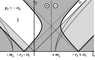
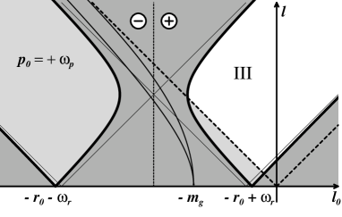
FIG. 4.: Allowed domains in the $(l_{o},l)$ plane for $p_{o}=\pm\omega_{p}$. The area shaded in dark gray is excluded by the delta function constraints. The areas shaded in light gray are above the light-cone (dotted lines). The light curves are the transverse and longitudinal mass shells of the thermalized gluon. The vertical dotted line is the separation between $\epsilon(p_{o})\epsilon(r_{o}+l_{o})=+1$ and $\epsilon(p_{o})\epsilon(r_{o}+l_{o})=-1$.

The regions on which we focus mostly in the following have been labeled by I, II and III. Looking at the signs of the quark momenta in each region, we can see that region I and III involve bremsstrahlung processes, while a new process appears in region II. This unexpected process can be described as a $q\bar{q}$ annihilation in which one of the fermions undergoes a scattering through a gluon exchange (see the figure 5).

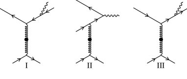
FIG. 5.: Physical processes included in the regions where $L^{2}<0$.

By the change of variables $P\to-R-L$, we can map the region I on the region III. As a consequence, the bremsstrahlung photon production can be obtained by looking only at the region III, and multiplying its contribution by an overall factor $2$.

D Collinear singularities

When both the external photon and the internal quark are massless, the diagrams of figure 3 display a collinear singularity when the 3-momentum of the quark is parallel to that of the emitted photon. Moreover, contrary to the collinear divergences encountered in the 1-loop contributions, which are at most logarithmic, we have here two denominators that can vanish almost simultaneously. This is of course obvious for the second diagram of figure 3 in which we have a double pole. But even for the first one, the poles are distinct but very close. Indeed, $R^{2}$ is vanishing when $\textstyle p$ is parallel to $\textstyle q$, while $(P+L)^{2}$ vanishes when $\mathchoice{{\hbox{\boldmath$\displaystyle r$}}}{{\hbox{\boldmath$\textstyle r$}}}{{\hbox{\boldmath$\scriptstyle r$}}}{{\hbox{\boldmath$\scriptscriptstyle r$}}}+\mathchoice{{\hbox{\boldmath$\displaystyle l$}}}{{\hbox{\boldmath$\textstyle l$}}}{{\hbox{\boldmath$\scriptstyle l$}}}{{\hbox{\boldmath$\scriptscriptstyle l$}}}$ is parallel to $\textstyle q$. As a consequence, when $\textstyle l$ is soft, these two conditions of collinearity are satisfied almost simultaneously, independently of the order of magnitude of the momentum $\textstyle q$. Therefore, the two denominators have very close poles, and their association mostly behaves like a double pole.

The collinear singularity of these diagrams is therefore quasi linear, instead of logarithmic. When the quark mass is taken into account, these divergences are regularized, but a consequence of their linear nature is the generation of powers of $1/g$. The strength of these divergences makes dominant the terms that have this configuration of quasi double poles. It is rather straightforward to show that this cannot occur when the gluon is time-like. Indeed, because of the delta function $\delta(P^{2}-M^{2}_{\infty})$, the denominator $(P+L)^{2}-M^{2}_{\infty}$ can approach zero only if $L^{2}<0$ for soft $L$. Therefore, we consider only the regions where $L^{2}<0$. It is easy to check that in the collinear limit, for soft $L$, the boundaries of region III are just $-l\leq l_{o}\leq l$, i.e. the inequality $|\cos\theta^{\prime}|\leq 1$ does not add any extra constraint beyond $L^{2}<0$.

E Soft photon production

Let me start with soft photons. I consider here photons having a small invariant mass $Q^{2}\ll q_{o}^{2}\ll T^{2}$. In this situation, it is easy to verify that the contribution of region II is subdominant, since the area of the phase space available to this process in the $(l_{o},l)$ plane is proportional to $q_{o}$. Moreover, for this region, the gluon momentum $L$ is necessarily hard, which implies that the two conditions of collinearity discussed above cannot be satisfied simultaneously. Therefore, bremsstrahlung is the only dominant process for the production of low invariant mass soft photons.

Using only the variables $u=1-\cos\theta$ where $\theta$ is the angle between $\textstyle p$ and $\textstyle q$, $p$, $l$ and $x=l_{o}/l$, we can write[9]

$$R^{2}-M^{2}_{\infty}\approx 2pq\left[u+{{M^{2}_{\rm eff}}\over{2p^{2}}}\right]\;,$$ (31)

where $M_{\rm eff}^{2}\equiv M^{2}_{\infty}+Q^{2}p^{2}/q_{o}^{2}$, and

$$\int\limits_{0}^{2\pi}\!\!\!{{d\phi}\over{(P+L)^{2}-M^{2}_{\infty}}}\approx{{2\pi(2pq)^{-1}}\over{\left[\left(u+{{M^{2}_{\rm eff}}\over{2p^{2}}}+{{L^{2}}\over{2p^{2}}}\right)^{2}-{{L^{2}}\over{p^{2}}}{{M^{2}_{\rm eff}}\over{p^{2}}}\right]^{1/2}}}\;,$$ (32)

where we performed the integration over the azimuthal angle $\phi$ between $\textstyle q$ and $\textstyle l$ at this stage since this denominator is the only place where $\phi$ appears at the dominant order. Among all the terms present in the amplitude, the only ones to be sensitive to the collinear singularity described in the previous section are those where two of these denominators are present. Other terms have a numerator that cancels one of the denominators, so that the collinear singularity is only logarithmic. On the basis of these considerations, it is easy to check that only the following term in $L^{2}$

$$-8L^{2}{{\overline{R}{}^{\rho}\overline{R}{}^{\sigma}+\overline{P}{}^{\rho}\overline{P}{}^{\sigma}}\over{\overline{R}{}^{2}(\overline{P+L}){}^{2}}}\;$$ (33)

is dominant.

It is then straightforward to perform the angular integration over $u=1$, to obtain the following expression of the imaginary part of the polarization tensor of the photon:

$$\hbox{\rm Im}\,\Pi^{{}^{RA}}{}_{\mu}{}^{\mu}(q_{o},{\mathchoice{{\hbox{\boldmath$\displaystyle q$}}}{{\hbox{\boldmath$\textstyle q$}}}{{\hbox{\boldmath$\scriptstyle q$}}}{{\hbox{\boldmath$\scriptscriptstyle q$}}}})\approx-\frac{e^{2}g^{2}N_{{}_{C}}C_{{}_{F}}}{3\pi^{2}}\frac{T^{3}}{q_{0}}(J_{{}_{T}}+J_{{}_{L}})$$ (34)

where we denoted

$$\!\!\!J_{{}_{T,L}}\equiv {6\over{\pi^{2}}}\int_{0}^{+\infty}dvv^{2}\,{e^{v}\over{(e^{v}+1)^{2}}}\int\limits_{0}^{1}\;\frac{dx}{x}\;|\widetilde{I}_{{}_{T,L}}(x)|$$ (36)

$$\times\int\limits_{0}^{+\infty}\;dw\;\frac{\sqrt{w/(w+4)}\hbox{\rm tanh}{}^{-1}\sqrt{w/(w+4)}}{(w+\widetilde{R}_{{}_{T,L}}(x))^{2}+(\widetilde{I}_{{}_{T,L}}(x))^{2}}\;,$$

with

$$v\equiv{p\over T}\;,\;\quad w\equiv{{-L^{2}}\over{M^{2}_{\rm eff}}}$$ (37)

$$\widetilde{I}_{{}_{T,L}}(x)\equiv{{\hbox{\rm Im}\,\Pi_{{}_{T,L}}(x)}\over{M^{2}_{\rm eff}}}\;,\;\quad\widetilde{R}_{{}_{T,L}}(x)\equiv{{\hbox{\rm Re}\,\Pi_{{}_{T,L}}(x)}\over{M^{2}_{\rm eff}}}\;.$$ (38)

A first noticeable feature of the result of Eq. (34) is its order of magnitude. Indeed, it is $1/g^{2}$ larger than 1-loop contributions calculated in [1, 2]. This is due to the strong collinear singularities described earlier.

The quantities $J_{{}_{T,L}}$ are coefficients quantifying the respective contributions of the transverse and longitudinal exchanged gluons. If we plot these quantities as a function of the parameter $Q^{2}/q_{o}^{2}$, we obtain the curves of figure 6. One can see that these coefficients are decreasing very fast if $Q^{2}$ increases. This is of course due to the fact that the invariant mass $Q^{2}$ attenuates the effect of the collinear singularities. What happens around $Q^{2}/q_{o}^{2}\sim 1$ will be presented in detail by H. Zaraket elsewhere in these proceedings [31].

FIG. 6.: Transverse and longitudinal contributions as a function of $Q^{2}/q_{o}^{2}$, for $3$ colors and $3$ light flavors. The value taken for the coupling constant is $g=0.44$.

Another feature of the result (34) is that it is totally free of any infrared divergence when the gluon momentum is going to zero, while one could have expected problems to occur with the transverse gluons (see the problems encountered in the calculation of the damping rate of a moving quark, for instance). If we look formally at the limit $M_{\infty}\to 0$ of the quantities $J_{{}_{T,L}}$ when $Q^{2}=0$, we find

$$\lim_{M_{\infty}\ll m_{\rm g}}J_{{}_{L}}\sim\ln(m_{\rm g}/M_{\infty})$$ (39)

$$\lim_{M_{\infty}\ll m_{\rm g}}J_{{}_{T}}\sim\ln(m_{\rm g}/M_{\infty})^{2}\;.$$ (40)

This result is interpreted as follows: the common power of the logarithm is due to the collinear singularity (common to both the transverse and longitudinal gluon contributions) which reappears when its regulator $M_{\infty}$ is suppressed. The reason why only a logarithm appears in this limit despite the fact that the singularity has been described earlier as quasi linear is precisely related to the fact that we don’t have exactly a double pole but two very close poles: the small separation between the two poles, which is responsible for extra powers of $1/g$, does not go to zero when $M_{\infty}\to 0$. In the transverse gluon contribution, there is an extra power of this logarithm which is interpreted as a remnant of an infrared singularity. To support this interpretation, we can introduce by hand a magnetic mass $m_{\rm mag}$ in the effective gluon propagator, and look at

$$\lim_{M_{\infty}\ll m_{\rm mag}\ll m_{\rm g}}J_{{}_{T}}\sim\ln(m_{\rm g}/M_{\infty})\ln(m_{\rm g}/m_{\rm mag})\;.$$ (41)

This limit indicates the infrared nature of the extra logarithm in the transverse gluon contribution. Equation (40) then tells us that the relevant regulator of this potential infrared singularity is the quark thermal mass when $M_{\infty}\gg m_{\rm mag}$, which can be understood in terms of phase space constraints. Indeed, if $L\to 0$ while $M_{\infty}>0$, the delta functions $\delta(R^{2}-M^{2}_{\infty})$ and $\delta((P+L)^{2}-M^{2}_{\infty})$ become incompatible with bremsstrahlung, which means that $M_{\infty}$ prevents the infrared singularity from having a support.

F Hard photon production

The calculation of 2-loop contributions to hard real photon production follows closely what has been done before for soft photons, at least for $Q^{2}=0$, a condition to which I will adhere in the following. Indeed, most of the aspects of the calculations were based on the fact that $Q^{2}\ll q_{o}^{2}$. Simply, since $\textstyle q$ cannot be neglected in front of $\textstyle p$, one must treat more carefully the angles between the various 3-vectors of the problem. If we still denote by $\theta$ the angle between $\textstyle p$ and $\textstyle q$, the angle $\theta^{\prime\prime}$ between $\textstyle q$ and $\textstyle l$ is now given by

$$\cos\theta^{\prime\prime}={{p}\over{r}}(\cos\theta\cos\theta^{\prime}+\sin\theta\sin\theta^{\prime}\cos\phi)+{{q}\over{r}}\cos\theta^{\prime}\;,$$ (42)

where $\theta^{\prime}$ and $\phi$ are defined in the same way as before. Then, it is easy to see that (31) is unchanged (except for the fact that $M^{2}_{\rm eff}$ becomes simply $M^{2}_{\infty}$ when $Q^{2}=0$), while (32) becomes

$$\int\limits_{0}^{2\pi}\!\!\!\!{{d\phi}\over{(P+L)^{2}-M^{2}_{\infty}}}\approx{{2\pi(p+q)(2qp^{2})^{-1}}\over{\left[\left(u+{{M^{2}_{\infty}}\over{2p^{2}}}+{{L^{2}}\over{2p^{2}}}\right)^{2}-{{L^{2}}\over{p^{2}}}{{M^{2}_{\infty}}\over{p^{2}}}\right]^{1/2}}}\;.$$ (43)

Again, the only dominant term in the matrix element is given by (33), which makes easy the evaluation of the bremsstrahlung contribution to hard real photons. We now obtain

$${\rm Im}\,\Pi^{{}^{AR}}{}_{\mu}{}^{\mu}(q_{o},\mathchoice{{\hbox{\boldmath$\displaystyle q$}}}{{\hbox{\boldmath$\textstyle q$}}}{{\hbox{\boldmath$\scriptstyle q$}}}{{\hbox{\boldmath$\scriptscriptstyle q$}}})\approx-{{e^{2}g^{2}NC_{{}_{F}}}\over{\pi^{4}}}{T\over{q_{o}^{2}}}(J_{{}_{T}}+J_{{}_{L}})$$ (44)

$$\times\int\limits_{0}^{+\infty}dp\,\left[{{p^{2}+(p+q_{o})^{2}}}\right]{{[n_{{}_{F}}(p)-n_{{}_{F}}(p+q_{o})]}}\;,$$ (45)

with now

$$J_{{}_{T,L}}=\int\limits_{0}^{1}{{dx}\over{x}}\,|\widetilde{I}_{{}_{T,L}}(x)|$$ (46)

$$\qquad\times\int\limits_{0}^{+\infty}dw\,{{\sqrt{w/{w+4}}\,{\rm tanh}^{-1}\sqrt{w/{w+4}}}\over{(w+\widetilde{R}_{{}_{T,L}}(x))^{2}+(\widetilde{I}_{{}_{T,L}}(x))^{2}}}\;.$$ (47)

As one can see, the structure of the bremsstrahlung contribution to the production of hard real photons is quite similar to the case of soft photons. In the above expressions, the coefficients $J_{{}_{T,L}}$ have been defined to match exactly those which have been defined previously, when $Q^{2}=0$. The only difference is in the integration over $p$ which is now more complicated because we cannot neglect $q_{o}$. The $q_{o}$ dependence that comes from this integral is non trivial now, but some limits are simple. In the limit $q_{o}\ll T$, we recover of course the result given for the production of soft real photons. A simple result can also be obtained in the opposite limit $q_{o}\gg T$, for which a simple expansion can be given for the integral over $p$, which leads us to

$${\rm Im}\,\Pi^{{}^{AR}}{}_{\mu}{}^{\mu}(q_{o},\mathchoice{{\hbox{\boldmath$\displaystyle q$}}}{{\hbox{\boldmath$\textstyle q$}}}{{\hbox{\boldmath$\scriptstyle q$}}}{{\hbox{\boldmath$\scriptscriptstyle q$}}})\approx-{{e^{2}g^{2}\ln(2)NC_{{}_{F}}}\over{\pi^{4}}}{T^{2}}(J_{{}_{T}}+J_{{}_{L}})\;.$$ (48)

As said before, the contribution of region II is negligeable only when $q_{o}$ is soft because of a small phase space, so that we must now take it into account. Its evaluation in the asymptotic region $q_{o}\gg T$ is very easy. Since $p_{o}=-\omega_{\mathchoice{{\hbox{\boldmath$\displaystyle p$}}}{{\hbox{\boldmath$\textstyle p$}}}{{\hbox{\boldmath$\scriptstyle p$}}}{{\hbox{\boldmath$\scriptscriptstyle p$}}}}$ in this region, we have instead of (31)

$$R^{2}-M^{2}_{\infty}\approx-2pq\left[v+{{M^{2}_{\infty}}\over{2p^{2}}}\right]\;,$$ (49)

where I denote $v\equiv 1+\cos\theta$. We can also check that (43) remains valid, except for the changes $u\to v$ and $p+q\to q-p$. The enhancement due to collinear singularities in the terms that contains these two denominators is unchanged near $v\sim g^{2}$. Concerning the boundaries of the integration domain, we can note that the statistical weight $n_{{}_{F}}(p_{o})-n_{{}_{F}}(p_{o}+q_{o})$ is equal to $1$ for $-q_{o}\leq p_{o}\leq 0$ and equals $0$ everywhere else (excepted in a small region of width $T$ where the transition from $1$ to $0$ takes place, but this provides corrections of relative order $T/q_{o}\ll 1$). For the $l$ and $x$ variables, the limits are $-1\leq x\leq 1$ and $0\leq l\leq l^{*}$ where the upper bound $l^{*}$ is always hard so that it can be taken to infinity without changing the result. Therefore, the integration over $x$ and $l$ gives again the same factor $J_{{}_{T}}+J_{{}_{L}}$ as in (48). Since the integration over $p$ is replaced now by

$$\int\limits_{0}^{q_{o}}dp(p^{2}+(q_{o}-p)^{2})={{2q_{o}^{3}}\over{3}}\;,$$ (50)

the contribution of region II for $q_{o}\gg T$ is

$${\rm Im}\,\Pi^{{}^{AR}}{}_{\mu}{}^{\mu}(q_{o},\mathchoice{{\hbox{\boldmath$\displaystyle q$}}}{{\hbox{\boldmath$\textstyle q$}}}{{\hbox{\boldmath$\scriptstyle q$}}}{{\hbox{\boldmath$\scriptscriptstyle q$}}})\approx-{{e^{2}g^{2}NC_{{}_{F}}}\over{3\pi^{4}}}{q_{o}T}(J_{{}_{T}}+J_{{}_{L}})\;.$$ (51)

It appears that the process of this region, behaving as $q_{o}T$ when $q_{o}\gg T$, instead of $T^{2}$ for bremsstrahlung, is the dominant one for the production of extremely hard photons.

IV Comparison with existing results

A Other thermal field theory approaches

The production rate of soft real photons has already been evaluated at 1-loop in thermal field theory by [1, 2]. The typical order of magnitude they found for the imaginary part of the photon polarization tensor is $e^{2}g^{4}\ln(1/g)T^{3}/q_{o}$, which means that the bremsstrahlung contribution found in (34) is larger by a factor $1/g^{2}$. Bremsstrahlung seems therefore to be the dominant process for the production of soft quasi-real photons. This extra $1/g^{2}$ factor can be traced back into the strong collinear singularity exhibited by bremsstrahlung processes. This effect can be seen as a breakdown of the effective expansion based on the resummation of hard thermal loops. Indeed, the powers of $1/g$ generated by these collinear divergences can change the order in $g$ of a contribution, so that the usual connection between the number of loops and the order in $g$ is lost.

Concerning hard real photons, [16, 30] calculated in thermal field theory the contribution of processes involving a time-like gluon, like Compton processes. Their calculation involves both 1-loop and 2-loop diagrams, and leads to

$${\rm Im}\,\Pi^{{}^{AR}}{}_{\mu}{}^{\mu}(q_{o},\mathchoice{{\hbox{\boldmath$\displaystyle q$}}}{{\hbox{\boldmath$\textstyle q$}}}{{\hbox{\boldmath$\scriptstyle q$}}}{{\hbox{\boldmath$\scriptscriptstyle q$}}})\approx-{{e^{2}g^{2}NC_{{}_{F}}}\over{16\pi}}{T^{2}}\ln\left({{cq_{o}}\over{\alpha_{{}_{S}}T}}\right)\;,$$ (52)

for $q_{o}\gg T$, where $c$ is a numerical constant equal to $0.23$. We are now in a position to compare the contributions given by bremsstrahlung, the $q\bar{q}$ annihilation appearing in region II, and the Compton processes calculated by Baier et al. For this comparison, we take $N=3$ colors and $N_{{}_{F}}=2$ light flavors, and a coupling constant $g=0.5$. At $Q^{2}=0$, the quantities $J_{{}_{T,L}}$ depend only on $N$ and $N_{{}_{F}}$, and are $J_{{}_{T}}\approx 4.45$ and $J_{{}_{L}}\approx 4.26$ with our choice of parameters. The evolution with the photon energy $q_{o}$ of these three contributions has been plotted on figure 7.

FIG. 7.: Comparison of various contributions to ${\rm Im}\,\Pi^{\mu}{}_{\mu}(Q)$ for a hard real photon.

We see that bremsstrahlung is dominating for the smaller values of $q_{o}$, while the region II becomes dominant for hard enough $q_{o}$. For intermediate energies, the three contributions are comparable. The sum of the three contributions is significantly above the Compton contribution considered alone.

B Connection with plasmon frequency calculations

In his talk [32], Flechsig presented results about the QCD plasmon frequency near the light-cone. This calculation is also plagued by very strong collinear singularities, very similar to those encountered in the real photon rate. A first sight, there is however a difference because the collinear singularities in the plasmon frequency arise already at one loop, and come from $ggg$ and $gggg$ effective vertices.

In order to make the connection between the present work and Flechsig’s approach, it is useful to note that at the level of the topologies, we have the following identity

(53)

between our diagrams and some 1-loop tadpole diagram. Indeed, the tadpole contains both the self-energy and the vertex topologies since there are several terms contributing to the $\gamma\gamma gg$ effective vertex, obtained by exchanging a photon and a gluon. Of course, the tadpole vanishes when one takes the trace over photon Lorentz indices, so that this equation does not reflect an exact algebraic identity between both sides (one would need to calculate the tadpole beyond the HTL approximation in order to be able to identify the two sides). Despite this limitation, one can note that both sides have the same denominators and therefore the same singularities. As a consequence, we can interpret our singularities as being collinear singularities encountered in hard thermal vertices when some external legs are on the light-cone[3] and conclude that the singularities encountered in our calculation are basically the same as those encountered by Flechsig. The only difference is that the HTL approximation makes the tadpole vanish when one traces it over the photon Lorentz indices, so that we have to go to two loops.

This remark suggests also a defect of the HTL approximation. Indeed, in the calculation of the tadpole of Eq. (53) the HTL approximation gives a zero coefficient to otherwise extremely singular (and large after regularization) terms. Therefore, it seems that the HTL approximation is not a good one in the presence of these strong collinear singularities, because one would need to go beyond this approximation to retain the relevant dominant terms in the tadpole.

C Semi-classical approach

Photon production by a plasma has also been studied by semi-classical methods in [4, 5, 6, 7]. Basically, in this approach, one studies the radiative energy loss of a fast quark undergoing multiple scatterings in a dense medium. The scattering centers are assumed to be static, which implies that the interaction is purely electric. This amounts to take only the longitudinal exchanged gluons into account. As a consequence, this interaction can be regularized by a Debye mass, and one does not have to worry about infrared divergences. In order to exhibit the analogy between this semi-classical approach and the thermal field theory, it is possible to write the bremsstrahlung contribution as given by (4) in thermal field theory in the following form

$$\left.{{dN}\over{dtd{\mathchoice{{\hbox{\boldmath$\displaystyle x$}}}{{\hbox{\boldmath$\textstyle x$}}}{{\hbox{\boldmath$\scriptstyle x$}}}{{\hbox{\boldmath$\scriptscriptstyle x$}}}}}}\right|_{\rm bremss}={{d{\mathchoice{{\hbox{\boldmath$\displaystyle q$}}}{{\hbox{\boldmath$\textstyle q$}}}{{\hbox{\boldmath$\scriptstyle q$}}}{{\hbox{\boldmath$\scriptscriptstyle q$}}}}}\over{(2\pi)^{3}2q_{o}}}\int{{d^{4}P}\over{(2\pi)^{4}}}\int{{d^{4}K}\over{(2\pi)^{4}}}\int{{d^{4}L}\over{(2\pi)^{4}}}$$ (54)

$$\quad\times\raise-19.91692pt\hbox to142.26378pt{\mbox{\epsfbox{fig07.ps}}}$$ (55)

$$\quad\times n_{{}_{F}}(r_{o}+l_{o})n_{{}_{F}}(k_{o})[1-n_{{}_{F}}(p_{o})][1-n_{{}_{F}}(k_{o}+l_{o})]$$ (56)

$$\quad\times 2\pi\delta(P^{2}-M^{2}_{\infty})\,2\pi\delta((R+L)^{2}-M^{2}_{\infty})$$ (57)

$$\quad\times 2\pi\delta(K^{2}-M^{2}_{\infty})\,2\pi\delta((K+L)^{2}-M^{2}_{\infty})\;,$$ (58)

where $R\equiv P+Q$. This kind of formula looks like the starting point of the semi-classical approach, but it differs from it by some essential aspects. The most important one is that it includes the contributions of the transverse exchanged gluons, which we have shown to be quite important since $J_{{}_{T}}$ is as large as $J_{{}_{L}}$. Neglecting it does not appear to be a good approximation. Moreover, this formula differs from the semi-classical ones by the details of how the Debye screening is incorporated in the gluon propagator. Indeed, the semi-classical approach just includes some constant Debye mass as a regulator, while in thermal field theory one takes into account all the momentum dependence of the gluon self-energy via the HTL resummation. Although this does not change significantly the physics, it may affect the numerical value of the production rate.

On the other hand, these simplifications allow the semi-classical method to handle more easily the multiple scatterings, and to show that some new collective phenomenon may appear. More precisely, multiple coherent scatterings may conspire in order to give a smaller photon production rate, a phenomenon known as the Landau-Pomeranchuck-Migdal effect [33, 34]. In order to extract this effect from thermal field theory, one should look at diagrams with two and more exchanged gluons.

V Conclusions and perspectives

In these proceedings, I have shown that 2-loop processes involving the exchange of a space-like gluon play a dominant role in the real photon production by a plasma. In particular, for the production of soft real photons, bremsstrahlung dominates over 1-loop contributions by a $1/g^{2}$ factor. Therefore, this study reconciliates thermal field theory with the semi-classical approach.

From a more formal point of view, this phenomenon is due to very strong collinear singularities in these processes. Although regularized by a thermal mass of order $gT$, an enhancement by a $1/g^{2}$ factor appears in the result as a remnant of these potential divergences. The possibility of such an enhancement can make certain contributions much larger than what one would have expected on the basis of their number of loops, therefore resulting in some kind of breakdown of the relationship between the order of magnitude and the number of loops. It would be very interesting to know if even stronger singularities can appear in higher order diagrams.

There are also other motivations to look at higher order topologies. Indeed, the LPM effect found in the semi-classical approach seems to indicate that equally important contributions come from the diagrams corresponding to photon emission induced by multiple scatterings. Moreover, the study of the effect of the thermal width made by [25, 26] seems also to indicate contributions from higher order diagrams.

REFERENCES

- [1] R. Baier, S. Peigné, D. Schiff, Z. Phys. C 62, 337 (1994).
- [2] P. Aurenche, T. Becherrawy, E. Petitgirard, Preprint ENSLAPP-A-452/93, hep-ph/9403320.
- [3] F. Flechsig, A.K. Rebhan, Nucl. Phys. B 464, 279 (1996).
- [4] J. Cleymans, V.V. Goloviznin, K. Redlich, Phys. Rev. D 47, 989 (1993).
- [5] J. Cleymans, V.V. Goloviznin, K. Redlich, Z. Phys. C 59, 495 (1993).
- [6] R. Baier, Y.L. Dokshitzer, A.H. Mueller, S. Peigné, D. Schiff, Nucl. Phys. B 478, 577 (1996).
- [7] R. Baier, Y.L. Dokshitzer, A.H. Mueller, S. Peigné, D. Schiff, Nucl. Phys. B 483, 291 (1997).
- [8] P. Aurenche, F. Gelis, R. Kobes, E. Petitgirard, Phys. Rev. D 54, 5274 (1996).
- [9] P. Aurenche, F. Gelis, R. Kobes, E. Petitgirard, Z. Phys. C 75, 315 (1997).
- [10] P. Aurenche, F. Gelis, R. Kobes, H. Zaraket, Phys. Rev D 58, 085003 (1998).
- [11] E. Braaten, R.D. Pisarski, Nucl. Phys. B 337, 569 (1990).
- [12] J. Frenkel, J.C. Taylor, Nucl. Phys. B 334, 199 (1990).
- [13] P. Aurenche, T. Becherrawy, Nucl. Phys. B 379, 259 (1992).
- [14] M.A. van Eijck, R. Kobes, Ch.G. van Weert, Phys. Rev. D 50, 4097 (1994).
- [15] E. Braaten, M. Thoma, Phys. Rev. D 44, 1298 (1991).
- [16] R. Baier, H. Nakkagawa, A. Niegawa, K. Redlich, Z. Phys. C 53, 433 (1992).
- [17] E. Braaten, R.D. Pisarski, Phys. Rev. D 45, 1827 (1992).
- [18] J. Frenkel, J.C. Taylor, Nucl. Phys. B 374, 156 (1992).
- [19] H. Schultz, Nuc. Phys. B. 413, 253 (1994).
- [20] H.A. Weldon, Phys. Rev. D 28, 2007 (1983).
- [21] C. Gale, J.I. Kapusta, Nucl. Phys. B 357, 65 (1991).
- [22] R.L. Kobes, G.W. Semenoff, Nucl. Phys. B 260, 714 (1985).
- [23] R.L. Kobes, G.W. Semenoff, Nucl. Phys. B 272, 329 (1986).
- [24] F. Gelis, Nucl. Phys. B 508, 483 (1997).
- [25] A. Niegawa, Phys. Rev. D 55, 4997 (1997).
- [26] A. Niegawa, Phys. Rev. D 56, 1073 (1997).
- [27] R.D. Pisarski, Physica A 158, 146 (1989).
- [28] H.A. Weldon, Phys. Rev. D 26, 1394 (1982).
- [29] N.P. Landsman, Ch.G. van Weert, Phys. Rep. 145, 141 (1987).
- [30] J.I. Kapusta, P. Lichard, D. Seibert, Phys. Rev. D 44, 2774 (1991).
- [31] H. Zaraket, These proceedings.
- [32] F. Flechsig, These proceedings.
- [33] L.D. Landau, I.Ya. Pomeranchuk, Dokl. Akad. Nauk. SSR 92, 535 (1953).
- [34] A.B. Migdal, Phys. Rev. 103, 1811 (1956).