Saclay-SPP, DESY 98

A Parametrisation of the Inclusive Diffractive Cross Section at HERA

Jochen Bartels

II. Institut für Theoretische Physik, Universität Hamburg,
Luruper Chaussee 149, D-22761 Hamburg

Christophe Royon

Service de Physique des Particules, DAPNIA, CEA-Saclay,
F91191 Gif sur Yvette Cedex, France

A recently proposed parametrization for the deep inelastic diffractive cross section is used to describe the H1 94 data. We find two possible solutions, and we discuss them is some detail.

1. Diffractive events at HERA  [1, 2] are generally attributed to the exchange of the Pomeron between the virtual photon and the proton. After the first observation of these events, attempts of a theoretical description  [3] where based upon the idea of Ingelman and Schlein  [4], and they viewed diffraction in deep inelastic scattering as “deep inelastic scattering on a Pomeron“. As a striking result along these lines, H1  [1] reported on a “hard gluon component of the Pomeron“ (where “hard“ refers to the behavior of the structure function near $\beta=1$). However, with increasing statistics both ZEUS and H1  [1, 2] found evidence that in DIS diffraction the Pomeron intercept tends to be higher than the soft hadronic Pomeron. This observation suggested that the diffractive cross section at HERA contains both a soft and a hard component, and the latter one is stronger than initially expected.

A theoretical description of the inclusive diffractive cross section, therefore, should contain both a nonperturbative Pomeron part and a perturbative contribution. As a possible strategy, one could start from that part of the final state where pQCD can be used safely, and then attempt to find a smooth extrapolation into the nonperturbative Regge region. As to the Pomeron, in the perturbative region it is most easily modelled by a two gluon-system, the gluon structure function of the proton. In the nonperturbative region, this model of a “hard Pomeron“ should smoothly connect with the soft hadronic Pomeron. Recently  [5] a parametrization of the diffractive cross section has been proposed which follows this line of arguments, and it has been applied to both ZEUS and H1 data. For the latter the kinematic region was restricted to those values of $\beta$, $Q^{2}$, and $x_{I\!\!P}$ for which also ZEUS data points exist. As a striking result, it was found that the ZEUS data allow for a unique and rather succesful description whereas for the H1 data two different fits of this model were found.

In the present paper we apply the parametrization of  [5] to the complete H1 94 data of the diffractive cross section. We confirm the existence of two different solutions and we study their properties in some detail.

Let us first briefly recapitulate the parametrization. It consists of 3 terms each of which stands for a particular diffractive final state:

$$F_{2}^{D(3),I}=A\left(\frac{x_{0}}{x_{I\!\!P}}\right)^{n_{2}}\beta(1-\beta)$$ (1)

$$F_{2}^{D(3),II}=B\left(\frac{x_{0}}{x_{I\!\!P}}\right)^{n_{2}}\alpha_{S}\left(ln(\frac{Q^{2}}{Q_{0}^{2}}+1)\right)(1-\beta)^{\gamma}$$ (2)

$$F_{2}^{D(3),III}=C\left(\frac{x_{0}}{x_{I\!\!P}}\right)^{n_{4}}\left(\frac{Q_{0}^{2}}{Q^{2}}\right)\left(ln(\frac{Q^{2}}{4Q_{0}^{2}\beta}+1.75)\right)^{2}\beta^{3}(1-2\beta)^{2}$$ (3)

where

$$n_{2,4}=n^{0}_{2,4}+n^{1}_{2,4}ln\left[ln\left(\frac{Q^{2}}{Q_{0}^{2}}\right)+1\right]$$ (4)

The first term describes the diffractive production of a $q\bar{q}$ pair from a transversely polarized photon, the second one the production of a diffractive $q\bar{q}g$ system, and the third one the production of a $q\bar{q}$ component from a longitudinally polarized photon. The ansatz for the $\beta$-dependence is motivated by rather general features of QCD-parton model calculations: At small $\beta$ (large diffractive masses $M_{X}$) the spin 1/2 (quark) exchange in the $q\bar{q}$ production (1) leads to a behavior $\sim\beta$, whereas the spin 1 (gluon) exchange in (2) corresponds to $\beta^{0}$. For large $\beta$ (small diffractive masses) in (1) and (3) calculations show  [6, 7] that pertubative QCD becomes reliable, and they lead to $1-\beta$ and $(1-\beta)^{0}$ in (1) and (3), resp. For the $q\bar{q}g$ term in (2) the situation is slightly more complicated: a QCD calculation  [8] leads to a $(1-\beta)^{3}$ behavior. But in view of the previous H1 result which suggests a hard gluon distribution inside the Pomeron and, therefore, also a large gluon contribution in $F_{2}^{D}$ near $\beta=1$, we will leave the exponent $\gamma$ as a free parameter. Comparing the behavior in $\beta$ near $1$ of the three terms we notice that the longitudinal term (3) dominates.

Turning to the $Q^{2}$ dependence, the first two terms are leading twist whereas the last one belongs to twist 4. Combining this with the $\beta$ dependence discussed before we see that the longitudinal term is important only near $\beta=1$. The $\ln Q^{2}$-terms follow from QCD-calcutions, and they indicate the beginning of the QCD $Q^{2}$-evolution. In the transverse case ((1) and (2)) the evolution starts only after the radiation of at least one gluon, whereas for the higher twist longitudinal case the first logarithm appears already in the quark loop. The longitudinal $q\bar{q}g$ production contributes to leading twist, but it does not have the $\log Q^{2}$ enhancement and therefore is small compared to the transverse term (2). It should be clear that the parametrization (1) - (3) does not yet aim at describing the $Q^{2}$ evolution over a large $Q^{2}$ region. At this early stage it is designed only for the small-x HERA region where $Q^{2}$ stays below $100$ GeV². The use in the large-$Q^{2}$ region will definitely require some refinement of the parametrization. Finally, the dependence on $x_{I\!\!P}$ cannot be obtained from perturbative QCD and therefore is left free. For the two transverse terms one expects approximately the same $x_{I\!\!P}$-behavior, not too far away from the soft Pomeron. For the longitudinal term (3), on the other hand, it has been shown  [7] that the $x_{I\!\!P}$ dependence should be approximately the same as for the square of the gluon structure function. In the fit both $n_{2}$ and $n_{4}$ are allowed to have have a linear rise in $\ln\ln Q^{2}$.

In contrast to the ZEUS diffraction data H1 data extend into the region of not so large rapidity gaps where, in the Regge language, also the exchange of secondary reggeons has to be taken into account. Within the spirit of the parametrization proposed in  [5] such a term is very natural: within pQCD it corresponds to the exchange of a $q\bar{q}$ system. Such a term has recently been studied in  [9]. In our present fit we follow the H1 procedure of  [1] and use the following ansatz:

$$F_{2}^{D(3),IV}(x_{I\!\!P},\beta,Q^{2})=Nf_{I\!\!R/p}(x_{I\!\!R})F_{2}^{I\!\!R}(\beta,Q^{2})$$ (5)

where the reggeon flux is taken to follow a Regge behaviour with a linear trajectory $\alpha_{I\!\!R}(t)=\alpha_{I\!\!R}(0)+\alpha^{{}^{\prime}}_{I\!\!R}t$ such that:

$$f_{I\!\!R/p}(x_{I\!\!P})=\int^{t_{min}}_{t_{cut}}\frac{e^{B_{I\!\!R}t}}{x_{I\!\!P}^{2\alpha_{I\!\!R}(t)-1}}dt$$ (6)

where $|t_{min}|$ is the minimum kinematically allowed value of $|t|$ and $t_{cut}=-1$ GeV² is the limit of the measurement and the values of $B_{I\!\!R}$ and $\alpha^{{}^{\prime}}_{I\!\!R}$ are fixed with hadron-hadron data [1]. $F_{2}^{I\!\!R}$ is assumed to be proportional to the pion structure function [10] . No interference is assumed between this reggeon exchange and the Pomeron exchange of (1) - (3). The presence of (5) is a new element in our fit.

In our fit the main parameters are the normalization constants A, B, C, N, and the exponent $\gamma$ of the $\beta$-dependence near $\beta=1$. Moreover, we allow the $x_{I\!\!P}$ exponents to vary, i.e. we have the five parameters $n_{2}^{0}$, $n_{2}^{1}$, $n_{4}^{0}$, $n_{4}^{1}$, and the intercept $\alpha_{R}(0)$ of the secondary. Finally, we also leave $x_{0}$ as a free parameter.

2. Let us now turn to the results of our fit (table 1). Most important, the data allow two different possible fits of the 1994 H1 data The parameter which distinguishes the two solutions is $\gamma$: in the first case we find $\gamma=8.24$, in the second case $\gamma=0.27$. Both solutions have an acceptable $\chi^{2}$ value, with a slight preference for the first one (high gamma). If we perform the fit with statistical errors only, the $\chi^{2}$ values per degree of freedom of the two fits are 1.10/df and 1.25/df, resp. An overall picture of the two solutions is given in Figures 1 and 2.

Table 1: Parameters obtained for the “perturbative gluon” (on the left) and “hard gluon” (on the right) solutions of the fit. The fits are performed with statistical and systematical errors added in quadrature. The two last fits are preformed imposing the $q\bar{q}g$ (B=0) or the longitudinal $q\bar{q}$ components to be zero (C=0). If the fits are performed with statistical errors only, the $\chi^{2}$ values for the perturbative gluon and for the hard gluon solutions are 236.0 (1.10/dof) and 269.1 (1.25/dof), resp.

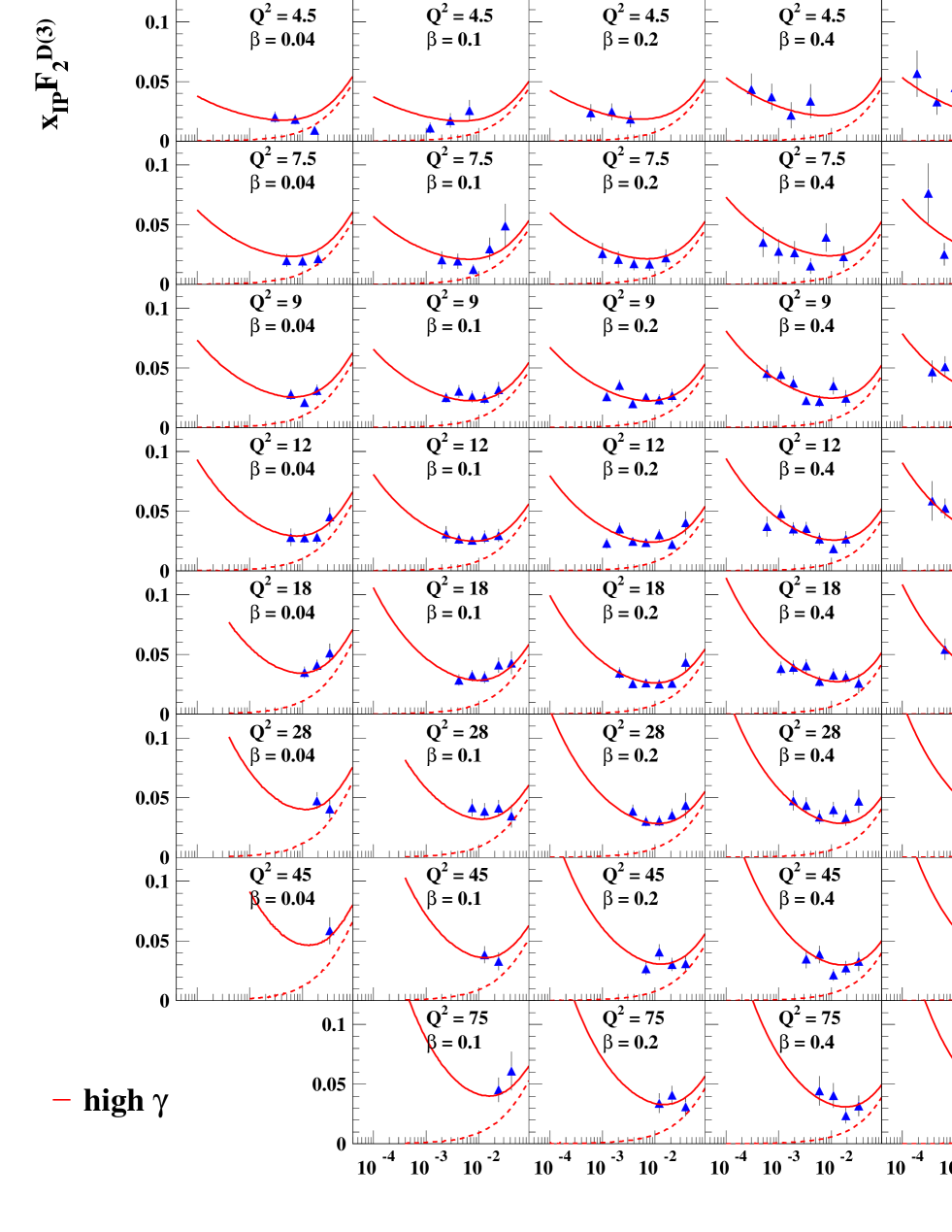
Figure 1: Result of the “perturbative gluon” fit. The triangles are the H1 1994 data. In full line is displayed the full result of the fit, and in dashed line, the reggeon component only which is important at low $\beta$ and high $x_{I\!\!P}$.

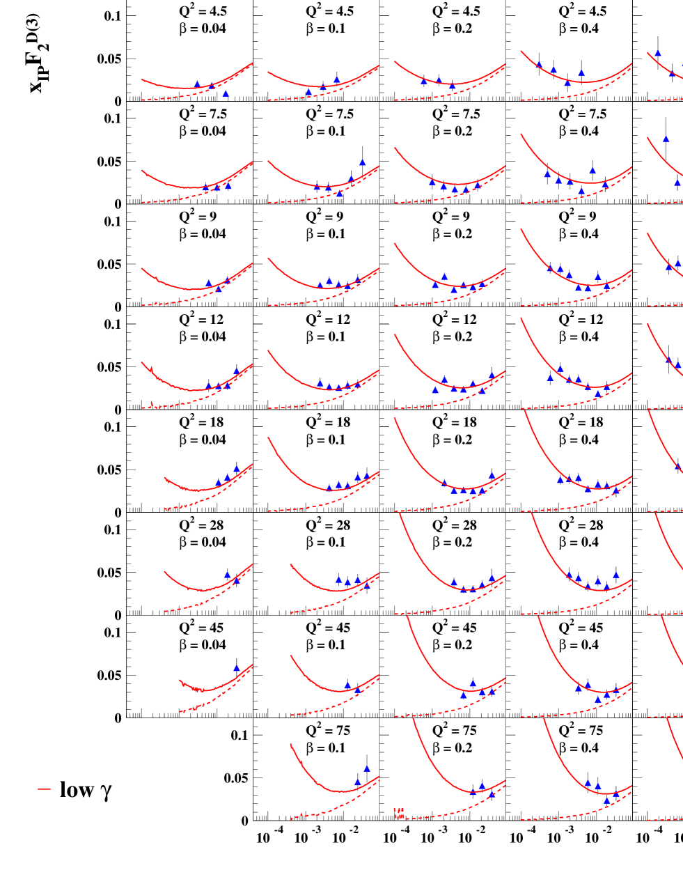
Figure 2: Result of the “hard gluon” fit. The triangles are the H1 1994 data. In full line is displayed the full result of the fit, and in dashed line, the reggeon component only which is important at low $\beta$ and high $x_{I\!\!P}$. This hard gluon fit is hardly distinguishable for the perturbative gluon one.

The difference between the two solutions is most clearly illustrated in Figs.3 and 4 where we plot the $\beta$-dependence of the different pieces (1) - (4). Data points lie mostly in the central and the rhs columns ($x_{I\!\!P}=0.001$ and $x_{I\!\!P}=0.01$), but for illustration we also extrapolate down to $x_{I\!\!P}=0.0001$. The main difference lies in the behavior of the $q\bar{q}g$ component: for the first solution ($\gamma=8.24$) it contributes only at small $\beta$ ($\beta<0.3$), whereas for the second one ($\gamma=0.27$) it extends up to $\beta$ near one. Qualitatively this second solution is close to the previous H1 solution with the hard gluon: the fact that the gluon distribution obtained from the H1 QCD analysis peaks near $1$ leads to a large gluon contribution to $F_{2}^{D}$ near $\beta=1$. In the following this solution to our fit will therefore be referred to as the “hard gluon” solution. The first solution, on the other hand, one is closer to the perturbative prediction which leads to $\gamma=3$. This solution will be called “perturbative gluon” solution in the following. For both solutions one sees that the transverse $q\bar{q}$ term has its maximum at medium $\beta$, and the longitudinal one contributes only near $\beta=1$. For the perturbative gluon solution the transverse $q\bar{q}$ is somewhat bigger than in the hard gluon case.

An important feature of both solutions is that none of the four components (1) - (4) comes out to be particularly small. To illustrate the importance of (2) and (3) we have repeated the fits (table 1) with putting either B or C equal to zero: in both cases the $\chi^{2}$ increases significantly. Let us notice that only one solution remains if $B=0$ is required (both solutions in Table 1 are identical). On the other hand, imposing $C=0$ in the hard gluon solution implies a very low value of $\gamma$ ($\gamma=0.001$), and so an important $q\bar{q}g$ term is present even at high $\beta$ and compensates the smallness of the $q\bar{q}$ term in this region. The situation changes if we impose the same kinematic cuts as used in the QCD fit of  [1]. Namely, by excluding the data points at high $y$ ($y>$0.45) and at low $M_{X}$ ($M_{X}<$2 GeV) this fit was restricted to the kinematic region where higher twist corrections are expected to be small. Also, only $\beta$ and $Q^{2}$ bins with more than three measured points were considered. Imposing the same cuts we have fitted our model to the data: we still find the two solutions. However, as expected, the longitudinal $q\bar{q}$ is now poorly constrained, and forcing the $C$ parameter to be 0 in the fit (excluding the higher twist contributions) does not change the quality of the fit very much (for the perturbative gluon solution the $\chi^{2}$ increases from 130 to 133, whereas for the hard gluon it remains unchanged ($\chi^{2}=$144)). The hard gluon solution now is even closer to the previous H1 solution in which no $q\bar{q}$ term was present.

The importance of the secondary reggeon term can be seen from Figs.1 and 2: in both cases its contribution becomes substantial only at low $\beta$ and large $x_{I\!\!P}$.

Scaling violations are illustrated in Figs.5 and 6. The $Q^{2}$ dependence of the longitudinal $q\bar{q}$ term (3) near $\beta=1$ is easily understood: it decreases with increasing $Q^{2}$, but the decrease is much slower than $1/Q^{2}$: this is due to the $(logQ^{2})^{2}$ enhancement in (3). As to the other two terms (1) and (2), there is an additional $Q^{2}$-dependence coming from the exponent $n_{2}$: in both fits $n_{2}^{1}$ is not small, and in combination with the rather large values of the ratio $x_{0}/x_{I\!\!P}$ it leads to a substantial increase with $Q^{2}$. In Figs.5 and 6 this explains why also the transverse $q\bar{q}$ component rises with $Q^{2}$. For the $q\bar{q}g$ component, which according to (2) has a logarithmic growth in $Q^{2}$, we see a difference between the two solutions: in the perturbative gluon solution it contributes only at small $\beta$. Consequently, the rise in $Q^{2}$ of $F_{2}^{D}$ is stronger at small $\beta$ than at larger $\beta$ (e.g. $\beta=0.65$). This effect is absent in the hard gluon solution, since here the gluon is present at all $\beta$.

In order to gain futher insight into the two solutions, we have also performed fits in a limited range in $\beta$ (or $M_{X}$). The parameters obtained for the perturbative gluon fit with cuts on $\beta$ in the data are given in Table 2. We note that the parameters are quite stable except for $\gamma$ which has the tendency to increase. However, the error on $\gamma$ is large, because we cut explicitely the region at low $\beta$ (or large $M_{X}$) where the $q\bar{q}g$ is significant. The hard gluon fit, on the other hand, is much less stable: already with the lowest cut at $\beta>0.1$ this solution disappears, and only the perturbative gluon solution remains. Cuts on $M_{X}$ in the data lead to the same results: excluding the high $M_{X}$ region, the perturbative gluon solution turns out to be stable, whereas a cut $M_{X}\leq 10$ is already enough to eliminate the hard gluon solution.

Figure 3: Display of the different components for the “perturbative gluon” fit. The transverse $q\bar{q}$ term belongs to the dashed line. The $q\bar{q}g$ term (dashed-dotted line) is important at low $\beta$, and the longitudinal $q\bar{q}$ term (dotted line) dominates at high $\beta$.

Figure 4: Display of the different components for the “hard gluon” fit. The transverse $q\bar{q}$ term belongs to the dashed line. The $q\bar{q}g$ term (dashed-dotted line) is not much $\beta$-dependent, and the longitudinal $q\bar{q}$ term (dotted line) dominates at high $\beta$.

Figure 5: Scaling violations in $\beta$ bins for a fixed value of $x_{I\!\!P}=0.003$ for the perturbative gluon (on the left) and hard gluon (on the right) solutions of the fit. The transverse $q\bar{q}$, $q\bar{q}g$, and longitudinal $q\bar{q}$ components are respectively in dashed, dashed-dotted and dotted lines, respectively. The full line is the sum of all components, including the secondary reggeon.

Figure 6: $\beta$-dependence of $F_{2}^{D}$ in bins of $Q^{2}$ at a fixed value of $x_{I\!\!P}=0.003$ for the perturbative gluon (on the left) and hard gluon (on the right) solutions of the fit. The dashed, dotted and dashed-dotted lines represent the transverse $q\bar{q}$, the longitudinal $q\bar{q}$ (important only at high $\beta$), and the $q\bar{q}g$ terms. The full line is the sum of all components, including the secondary reggeon.

	standard	$\beta>0.0.04$	$\beta>0.1$	$\beta>0.2$	$\beta>0.4$
$\gamma$	8.24 $\pm$ 1.06	11.3 $\pm$ 2.2	15.2 $\pm$ 5.2	20. $\pm$ 18.	20. $\pm$ 17.
$A$	0.056 $\pm$ 0.005	0.048 $\pm$ 0.012	0.048 $\pm$ 0.007	0.051 $\pm$ 0.005	0.056 $\pm$ 0.005
$B$	0.025 $\pm$ 0.003	0.030 $\pm$ 0.011	0.072 $\pm$ 0.080	0.085 $\pm$ 1500.	0.83 $\pm$ 9800.
$C$	0.035 $\pm$ 0.016	0.040 $\pm$ 0.018	0.037 $\pm$ 0.018	0.036 $\pm$ 0.016	0.044 $\pm$ 0.018
$\chi^{2}$	184.6	170.9	150.4	117.7	79.2

Table 2: Parameters obtained for the perturbative gluon solution of the fit after different cuts on $\beta$ in the data.

3. Next we use our ansatz (1) - (4) for the ZEUS 94 data  [2]. In agreement with  [5] we find only one solution, and the $\gamma$-value turns out to be identical: $\gamma\sim 4.3$. Comparing this solution with the perturbative gluon solution of our H1 fit, we find that they are very similar, both qualitatively and quantitavely. For instance, if in the H1 fit we fix $\gamma$ at the ZEUS value $\gamma=4.3$, we get a $\chi^{2}$ of 197.8 which is not much bigger than the $\chi^{2}$ of the fit with all parameters left free ($\chi^{2}=186.7$). As an important result of our ZEUS fit, we note that the fit is not improved by adding the secondary reggeon: the reggeon normalisation is found to be compatible with zero. This shows that ZEUS data do not require any secondary contribution.

To obtain a better understanding of the differences between the fits to the H1 data and to the ZEUS data  [2] , we have tried to compare the result of the H1 fit (the perturbative gluon solution) with the ZEUS data. The result is shown in Fig.7. The triangles represent the recently published ZEUS data, and the squares the H1 data. To be able to compare directly H1 and ZEUS data, we had to shift the H1 data to the $Q^{2}$ and $\beta$ ZEUS bins, using the perturbative gluon solution of the fit. Let us notice that this comparison does not depend much on the way we perform the extrapolation, as the $Q^{2}$ and $\beta$ bins from H1 and ZEUS are rather close. Further more, an extrapolation using a completely different fit based on the dipole model give the same interpolated values [12]. The full curve is then the perturbative gluon fit result with H1 data. The hard gluon solution restricted to the ZEUS bins would be indistinguishable on this plot. The dashed line denotes the result of our fit to the ZEUS data. We notice that the fits differ precisely in that region where one sees differences in the data, more precisely in the bins $\beta=$0.2, $Q^{2}$=8, and, $\beta=$0.7, $Q^{2}=$60 [12]. The differences in the fit parameters are clearly due to differences in the data points. More precise data in these regions will be thus very useful.

Figure 7: Comparison between H1 (squares) and ZEUS data (triangles). The full line represents the H1 perturbative gluon fit, and the dashed line our ZEUS fit. We notice that the differences in the fits are precisely in the region where the data differ.

4. So far we have not discussed our results for the exponents $n_{2}$ and $n_{4}$. Since the errors for these parameters are not small, one may feel that at this stage we should not attribute too much weight to them. Nevertheless, in the following we describe a few fits in which we impose constraints on $n_{2}$ and/or $n_{4}$. First we try to identify the $x_{I\!\!P}$ dependence in (1) and (2) with the soft Pomeron, leaving $n_{4}$ as a free parameter. We put $n_{2}=1.12$ (this differs from the soft Pomeron value $2\alpha_{I\!\!P}(0)-1=1.16$ by a small amount which is due to the integral over the momentum transfer $t$) and $n_{2}^{1}=0$, i.e. we exclude any $Q^{2}$ variation. The results for both solutions are shown in table 3. The obtained $\chi^{2}$ are quite bad: 254.2 (291.2) to be compared with 206.8 (184.6) in table 1 for the perturbative (hard) gluon solutions. This makes it unlikely that the diffractive structure function data could be described by the soft pomeron. In a variant of this test we have also treated $n_{2}^{0}$ as a free parameter (still keeping $n_{2}^{1}=0$). For the perturbative gluon solution we find a reasonable fit ($\chi^{2}=221.9$) for $n_{2}^{0}=1.38$, and for the hard gluon solution the fit gives $n_{2}^{0}=1.23$ with $\chi^{2}=239.6$.

Next we test the possibility of identifying the $x_{I\!\!P}$ dependence of the longitudinal term with the gluon density in the proton. We take the gluon parametrisation from [14] which is known to give a good description of the proton structure function data measured at HERA and fit it to the form $x^{-\alpha+1}$. We find

$$xG\sim x^{-\alpha+1}=x^{-0.18-0.15\ln(\ln(Q^{2})+1)}$$ (7)

where the scale of $Q^{2}$ is 1 GeV². This suggests to parametrize the exponent $n_{4}$ in the following way:

$$n_{4}=2\alpha-1=1.45+0.17\ln\left(\ln(\frac{Q^{2}}{Q_{1}^{2}})+1\right).$$ (8)

The result of both the perturbative gluon solution and the hard gluon solution are given in Table 3 (middle columns). We note that the quality of the fits is about the same as those obtained in Table 1. The transverse terms prefer a soft Pomeron with a rather strong $Q^{2}$ dependence of the exponent $n_{2}$. We also observe that, for the hard gluon solution, the value of the parameter $x_{0}$ is quite different from the fit in table 1 (cf. the footnote on p.2). We conclude that both solutions are consistent with the theoretical expectation that the longitudinal part of our parametrization is hard, i.e. its energy dependence can be described by the gluon structure function.

We have also tested the possibility of identifying the $x_{I\!\!P}$ dependence of the longitudinal term with the structure function $F_{2}$ of the proton. It has been shown  [13] that the $F_{2}$ slope in $x$ can be parametrised as follows:

$$\alpha=\frac{d\ln F_{2}}{dln1/x}=1.15+0.09\log_{10}Q^{2},$$ (9)

where the scale of $Q^{2}$ is $1$ GeV². The exponent $n_{4}$ can then be expected to vary as

$$n_{4}=2\alpha-1=1.31+0.18\log_{10}\frac{Q^{2}}{Q_{1}^{2}}$$ (10)

In our fit we put the scale $Q_{1}^{2}=1$GeV². The results are shown in the righmost column of Table 3. Again, the transverse terms in our parametrization want to have a soft Pomeron with a rather large $Q^{2}$ dependence. The quality of the fits is about the same as that of the first fits in Table 1. Changing the scale to $Q_{1}^{2}=4$GeV² or treating it as a free parameter does not change the result very much. Alltogether, the parameters of these fits are very similar to the previous one with the gluon structure function.

Table 3: Parameters obtained for the perturbative gluon (on the left) and hard gluon (on the right) solutions of the fit. The first fit is obtained by imposing the value of the soft pomeron exponent for $n_{2}$ and in the second and third fit respectively, $n_{4}$ follows the gluon slope in $x$ and the $F_{2}$ slope in $\log 1/x$ (cf text).

5. We conclude with a few general comments. Within the parametrization suggested in  [5] have tried to clarify the differences between the two possible solutions for the H1 94 data, and their relation to the previously reported H1 solution with the hard gluon. One of the two solutions (named ‘perturbative gluon‘) is closer to what one expects from a straightforward extrapolation of perturbative QCD calculations, whereas the other one (called ‘hard gluon‘) is closer to the previous H1 result. The main difference lies in the $\beta$ dependence of the $q\bar{q}g$ contribution. Apart from a small difference in $\chi^{2}$ (in favor of the perturbative gluon solution), we also found some evidence that, when we impose kinematic cuts on the data the hard gluon solution is slightly less stable than the perturbative gluon solution.

As we have discussed in the beginning of this letter the parametrization for $F_{2}^{D}$ is based upon an attempt to interpolate between the QCD parton model (hard region) and Regge physics (soft Pomeron). In this first step of testing this approach we have given much freedom to our parametrization. In a future step it will be interesting to see how specific final states fit into this parametrization and maybe used to constrain the parameters of our fit. Two obvious candidates are the production of longitudinal vector mesons which should be contained in the third term of our parametrization, and the production of $q\bar{q}$ jets (contained in the first term) and $q\bar{q}g$ jets (inside the second term) from the transverse photon. The measured cross sections of these final states and a careful analysis of their topological features could be used to estimate the parameters of our ansatz. Moreover, their measurement can decide which of the two solutions discussed in this letter is to be preferred.

Acknowledgement: We thank J.Dainton for a careful reading of our manuscript and for his helpful criticism. We also thank R.Peschanski for a careful reading of the manuscript.

Note added in proof: Another fit of our model to the combined 94 and the (preliminary) 95 low $Q^{2}$ data of H1 has been presented at the Brussels DIS98 (Talk presented by T.Nicholls) conference. The extrapolation into the region of smaller $Q^{2}$ values works quite reasonably. More recently (H1 Collab., Contribution to ICHEP98, Vancouver, July 98), our fit has been extrapolated also into the large $Q^{2}$ region ($200$ GeV² $<$ $Q^{2}$ $<$ $800$ GeV²). We feel rather hesitant in using our simple parametrization in this region. First, as we have said before, extending the $Q^{2}$ region in such a dramatic way our parametrization needs more terms and a more accurate way of handling the $Q^{2}$ evolution. Secondly, in the large $Q^{2}$ region region of HERA $x_{I\!\!P}$ is not really small, and the influence of the secondary exchange term (4) of our parametrization starts to dominate. Comparison of our fit with the large-$Q^{2}$ data, therefore, does not only test the $Q^{2}$ evolution of our parametrisation but also of the pion structure function used in the fit.

1 References

References

- [1] H1 coll., Z.Phys. C76 (1997) 613.
- [2] ZEUS coll., Eur. Phys. J. C1 (1998) 81.
-
[3]
K.Golec-Biernat and J.Kwiecinski, Phys.Lett. B 353
(1995) 329;
T.Gehrmann and W.J.Stirling, Z.Phys. C 70 (1996) 89;
H1 coll., Z.Phys. C76 (1997) 613. - [4] G. Ingelman, P. Schlein, Phys. Lett. B152 (1985) 256.
- [5] J. Bartels, J. Ellis, H. Kowalski, M. Wüsthoff, hep-ph/9803497 and to be published in Eur.Phys.J.
-
[6]
A.Donnachie and P.V.Landshoff, Phys.Lett.
B 191(1987) 309;
N.N.Nikolaev and B .G.Zakharov, Z.Phys.C 53 (1992) 331. - [7] J.Bartels, H.Lotter, and M.Wüsthoff, Phys.Lett. B379 (1996) 239; Erratum ibid. B 232) (1996) 449.
- [8] M.Wüsthoff, PhD Thesis, University of Hamburg, DESY 95-166.
- [9] W.Schäfer, hep/ph-9806295.
- [10] M. Glück, E. Reya, A. Vogt, Z.Phys. C53 (1992) 651.
- [11] J. F. Owens, Phys. Rev. D30 (1984) 943.
- [12] A. Bialas, R. Peschanski, Ch. Royon, Phys. Rev D57 (1998) 6899; S.Munier, R.Peschanski, C.Royon, to be published in Nucl.Phys.B, hep-ph/9807488
- [13] H1 coll., Nucl.Phys. B470 (1996) 3; L.Schoeffel, Ph. D. Thesis, University of Orsay, unpublished.
- [14] M. Glück, E. Reya, A. Vogt, Z. Phys. C67 (1995) 433.