Non-Equilibrium Dynamics with Fermions on a Lattice in Space and Time

Abstract

We consider the dynamics of the $1+1$ dimensional abelian Higgs model with axially coupled fermions, in the large $N_{f}$ limit, on a lattice in space and real-time. We allow for inhomogeneous classical Bose fields. In order to deal with the lattice doublers, we use Wilson’s lattice fermions. The lattice formulation leads to a stable integration algorithm. We illustrate the implementation with numerical results.

I Introduction

Real-time dynamics of quantum fields plays an important role in the early universe, in heavy ion collisions and in condensed matter. For example, a detailed understanding of the rate of sphaleron transitions at high temperature is relevant for baryogenesis. This is a non-perturbative problem, which should be treated preferably directly in real-time.

However, as is usually the case, in order to do actual calculations, approximations have to be made. The classical approximation [1, 2, 3, 4, 5] is based on the observation that at sufficiently high temperature the relevant long distance modes in the quantum theory behave classically. Hence it makes sense to study the classical equations of motion. The advantage is that it is (almost) straightforward to implement it numerically, and that e.g. sphaleron transitions are easy to find. However, it has become clear that Hard Thermal Loop (HTL) effects play an important role, and that it is necessary to incorporate them in a classical field and/or classical particle approach [6, 7].

Other possibilities are large $N$ or Hartree approximations [8, 9, 10, 11], which have been applied to e.g. (inflationary) scalar models and gauge theories. In this formulation the fields are split in a classical part and a quantum field, and they are coupled via semiclassical equations of motion, which are exact in the limit $N\to\infty$. The advantage is that quantum effects, including the backreaction on the classical fields, are taken into account. However, in actual numerical calculations, the emphasis has been on the case of homogeneous classical fields [10, 11]. This excludes inhomogeneous classical field configurations, such as the sphaleron.

Since we want to improve both the classical approximation by including quantum effects (such as HTL’s in $3+1$ dimensions) and the large $N$ approach by relaxing the classical field being homogeneous, we consider here the second approach with inhomogeneous classical fields.

After a discussion of the model, we describe the effective equations of motion. They are defined on a lattice in space and time, to have gauge invariance and numerical stability. We illustrate this with some numerical results.

II Abelian Higgs model with axially coupled fermions

We consider the abelian Higgs model in $1+1$ dimensions, with axially coupled fermions. The (continuum) action is

$$S=-\int d^{2}x\Big{[}\frac{1}{4e^{2}}F_{\mu\nu}F^{\mu\nu}+|D_{\mu}\phi|^{2}+\lambda(|\phi_{x}|^{2}-\frac{1}{2}v^{2})^{2}$$

$$+\bar{\psi}(/\!\!\!\partial+\frac{1}{2}i/\!\!\!\!A\gamma_{5})\psi+G\bar{\psi}(\phi^{*}P_{L}+\phi P_{R})\psi\Big{]}.$$

It has a number of properties in common with the Standard Model. The bosonic vacuum is non-trivial, and is labeled with the Chern-Simons number $C=-\int dx^{1}A_{1}/2\pi$, being integer at a vacuum. The vacua are separated by a finite energy sphaleron barrier, where $C$ is half integer. There is a global vector symmetry, $\psi\to e^{i\xi}\psi$, which leads to a classically conserved vector current $j^{\mu}_{f}=i\bar{\psi}\gamma^{\mu}\psi$. However, the corresponding charge, the fermion number $Q_{f}=\int dx^{1}j^{0}_{f}$, is not conserved in the quantum theory, because of the anomaly: $Q_{f}(t)-Q_{f}(0)=-(C(t)-C(0))$. The bosonic part of this model has been used before to test the classical approximation [2, 3].

Being in $1+1$ dimensions has a few consequenses. The typical HTL expressions are subdominant, so that these play a less important role [3]. Also the divergences are less severe, only the Higgs self energy is divergent, and only due to Higgs and fermion one loop contributions. And it is much easier to deal with numerically than $3+1$ dimensional models.

III On the lattice in real-time

In order to formulate the model on a lattice, it is convenient to first put the model in a more suitable form. By performing charge conjugation on the right-handed fermions only, $\psi_{R}\to(\bar{\psi}_{R}{\cal C})^{T},\psi_{L}\to\psi_{L}$, where ${\cal C}$ is the charge conjugation matrix, we write the model as one with a vector gauge symmetry. The fermionic part of the action becomes the usual Schwinger model with a Majorana-like Yukawa coupling

$$S_{f} = -\int d^{2}x\Big{[}\bar{\psi}(/\!\!\!\partial-\frac{1}{2}i/\!\!\!\!A)\psi$$

$$\;\;\;\;\;\;\;\;+\frac{1}{2}G\psi^{T}{\cal C}^{\dagger}\phi^{*}\psi-\frac{1}{2}G\bar{\psi}{\cal C}\phi\bar{\psi}^{T}\Big{]}.$$

The anomalous current is now axial, $j^{\mu}_{5}=i\bar{\psi}\gamma^{\mu}\gamma_{5}\psi$, and the anomaly equation reads

$\displaystyle Q_{5}(t)-Q_{5}(0)=C(t)-C(0).$

Since the Yukawa term has become Majorana-like, it is convenient to work with a real 4-component Majorana field $\Psi$.

It is now straightforward to put this theory on a space-time lattice with lattice spacing $a_{0},a_{1}=a$, using Wilson’s lattice fermions, known from euclidean lattice field theory. Lattice equations of motion and currents associated to global symmetries follow in the usual way.

IV Effective equations of motion

Effective equations of motion can be derived by considering $N_{f}$ fermion fields with $N_{f}\to\infty$. After integrating out the fermions and rescaling $\phi$ and $v$ with $\sqrt{N_{f}}$, $e$ and $G$ with $1/\sqrt{N_{f}}$, and $\lambda$ with $1/N_{f}$, the resulting bosonic effective action is proportional to $N_{f}$, and the remaining bosonic path integral can be approximated with a saddle point expansion. In leading order this results in the semiclassical Maxwell-like equations of motion [9]. In this approximation, the Bose fields are treated as classical fields, and the fermions, that are fully quantized, live in their background. The initial conditions for the original (unscaled) $\phi$ and $eA_{\mu}$ have evidently to be such that they are of order $\sqrt{N_{f}}$.

When the classical field is constrained to be homogeneous, the quantum fluctuations are treated in practise with a mode function expansion [10, 11]. Since we want to allow also inhomogeneous Bose fields, we use a ’generalized’ mode function expansion, i.e. at $t=0$, the fermion field is expanded in plane waves in order to be able to specify the initial quantum state, but for $t>0$ the space dependence is determined by the field equations. The result is that the mode functions have both a momentum label $p$ corresponding to the initial state, and a general space (and time) dependence, written as $x=(t,x^{1})$.

We expand the field as

$\displaystyle\Psi_{x}=\frac{1}{\sqrt{L}}\sum_{p,\alpha}\left[b_{p}(\alpha)w_{p}(x;\alpha)+b^{\dagger}_{p}(\alpha)w^{*}_{p}(x;\alpha)\right],$

with the initial condition

$\displaystyle w_{p}(t=0,x^{1};\alpha)=e^{ipx^{1}}w_{p}(\alpha).$

$w_{p}(\alpha)$ is an eigenspinor of the Dirac hamiltonian at $t=0$, and $\alpha=\{+,-\}$ labels the independent eigenspinors. Expectation values of the time independent creation and annihilation operators $b_{p}^{(\dagger)}(\alpha)$ specify the quantum state at $t=0$. We take either a vacuum or a thermal initial state, summarized by $\sigma_{p}(\alpha)\equiv\langle[b_{p}(\alpha),b_{p}^{\dagger}(\alpha)]\rangle=1-2f_{p}(\alpha)$, with $f_{p}$ the Fermi-Dirac distribution.

The bosonic equations are (in the temporal gauge $A_{0}=0$)

$$\partial^{\prime}_{0}\partial_{0}A_{1x}=e^{2}(j_{h_{x}}^{1}+\langle j_{f_{x}}^{1}\rangle),$$

$$\partial^{\prime}_{1}\partial_{0}A_{1x}=-e^{2}(j_{h_{x}}^{0}+\langle j_{f_{x}}^{0}\rangle),$$

$$\partial^{\prime}_{0}\partial_{0}\phi_{x}=D^{\prime}_{1}D_{1}\phi_{x}-2\lambda(|\phi_{x}|^{2}-\frac{1}{2}v^{2}_{B})\phi_{x}+G\langle F_{x}\rangle.$$

The second equation is Gauss’ law. The (primed) derivatives denote forward (backward) lattice derivatives. $j_{h}^{\mu}$ is the classical Higgs contribution to the current.

The fermion current $\langle j_{f}^{\mu}\rangle$ and force due to the fermions on the scalar field $\langle F\rangle$ can be written in terms of mode functions. The mode functions themselves obey the lattice Dirac equation in the presence of the Bose fields. This gives a closed set of equations.

Also observables such as the fermion vector and axial charge are expressed in terms of the mode functions. As an example, we show here the axial charge density $\langle j^{0}_{5_{x}}\rangle$ on the lattice

$$\langle j^{0}_{5_{x}}\rangle = -\frac{1}{4L}\sum_{p,\alpha}\sigma_{p}(\alpha)\Big{[}w_{p}^{\dagger}(t,x^{1};\alpha)\gamma_{5}\rho_{2}w_{p}(t+a_{0},x^{1};\alpha)$$ (2)

$$\;\;\;\;\;+w_{p}^{\dagger}(t+a_{0},x^{1};\alpha)\gamma_{5}\rho_{2}w_{p}(t,x^{1};\alpha)\Big{]}.$$

Here $\rho_{2}$ is a matrix appearing in the Majorana description.

The equations of motion still contain the divergence of the quantum theory. Since we only integrated out the fermions, and we treat the scalar field completely classical, only the fermion loop divergence enters in the equations. $\langle F_{x}\rangle$ is a logarithmically divergent sum. It’s divergence is canceled with the appropriate bare $v_{B}^{2}$.

V Numerical results

We have used the following initial conditions. The initial fermion mode functions are eigenspinors of the Dirac hamiltonian in the presence of a vacuum configuration of Bose fields, i.e. $A_{1}=0,\phi=v_{R}/\sqrt{2}$, and we take a vacuum initial state for the creation and annihilation operators, i.e. $\sigma_{p}(\alpha)=1$. The Higgs field is initially homogeneous, $\phi=v_{R}/\sqrt{2}$, but for its time derivative, $\partial_{0}\phi=\pi$, only the low momentum modes have a non-zero amplitude. The high momentum modes of $\pi$ are initially zero. This makes the classical field inhomogeneous. Both the Chern-Simon number and its time derivative have a non-zero value at $t=0$. The initial configuration is chosen in such a way that it obeys Gauss’ law. This completely specifies the spatial dependence of $\partial_{0}A_{1}$.

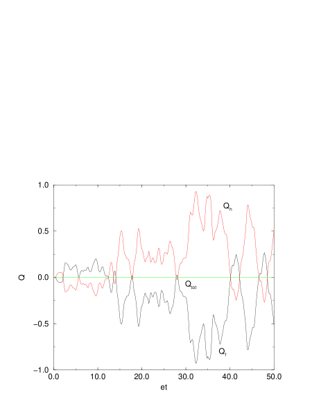
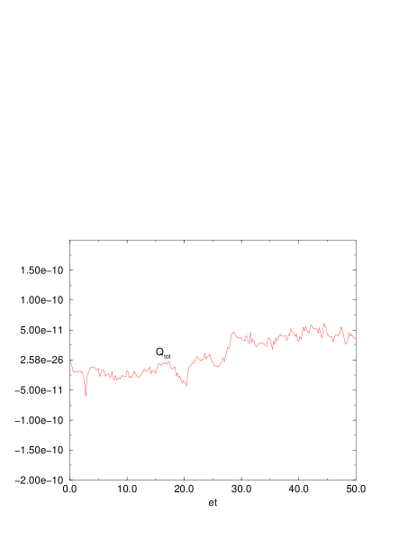
FIG. 1.: $Q_{h}$, $Q_{f}$ and $Q_{\rm tot}=Q_{f}+Q_{h}$ versus $et$.

FIG. 2.: Total conserved charge $Q_{\rm tot}$ versus $et$.

The quantum divergence in the equations is treated in the following way. The renormalized Higgs expectation value $v_{R}$ is fixed, and then the corresponding bare $v_{B}$ is determined using the equation for the scalar field at $t=0$. We checked that this leads to convergent physical results when the lattice spacing $a$ is made smaller.

Every dimensionful parameter is written in units of $e$. The parameters are $\lambda/e^{2}=G/e=0.25$ and the renormalized Higgs expectation value is $v_{R}^{2}=10$. The physical size is $eL=3.2$ ($L=aN$). Furthermore, the temporal lattice spacing $a_{0}/a=0.01$, and the number of lattice points $N=64$.

We now discuss the numerical results. Gauss’ law demands that the total charge $Q_{\rm tot}(t)=Q_{h}(t)+Q_{f}(t)$ is zero. Our initial conditions are such that both the Higgs charge, $Q_{h}(0)$, and the fermion charge, $Q_{f}(0)$, are separately zero. Under real-time evolution, having an inhomogeneous system, the individual charges do not stay zero, but the sum vanishes (up to machine precision). This is demonstrated in Figs. 2, 2. Since we solve a large set of partial differential equations (in particular there is an equation for every mode function, and there are $2N$ mode functions), this is non-trivial.

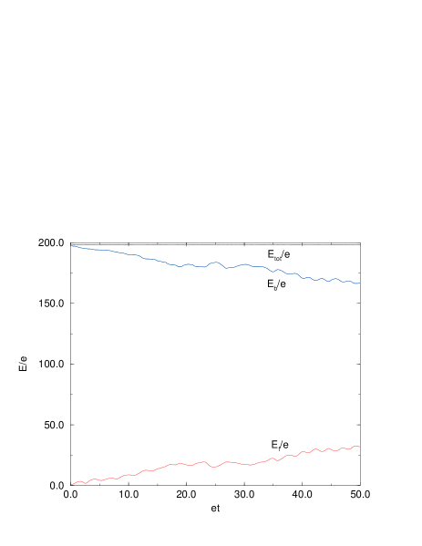
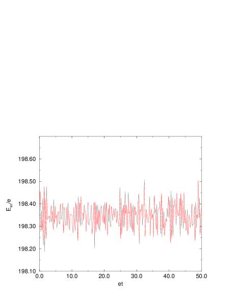
FIG. 3.: Bosonic energy, $E_{b}/e$, fermionic energy, $E_{f}/e$, and total energy $E_{\rm tot}/e=(E_{b}+E_{f})/e$ versus $et$.

FIG. 4.: Total conserved energy $E_{\rm tot}/e$ versus $et$.

Also the total energy $E_{\rm tot}=E_{b}+E_{f}$ is conserved, but not to such high accuracy as the charge. This is shown in Figs. 4, 4. The fermions are initialized in a vacuum state ($E_{f}(0)=0$). All the initial energy is contained in the low momentum modes of the Bose fields. This is clearly a non-equilibrium situation, and energy is transferred into the fermion degrees of freedom during time evolution.

Interesting observables are the Chern-Simons number $C$ and the anomalous axial charge $Q_{5}$. According to the anomaly equation, these should be equal during time evolution. $C$ is a ’simple’ observable in the sense that it is just the sum of $A_{1}$ over all lattice points. On the contrary, $Q_{5}$ is obtained by taking the sum over inner products between all modes functions, see (2). Results are given in Fig. 6. It shows that $Q_{5}$ follows $C$ at early times, in agreement with the anomaly equation. For later times they start to deviate. This is an artefact of the lattice discretization, which is reduced by taking smaller lattice spacing. In Fig. 6 we show the Higgs order parameter.

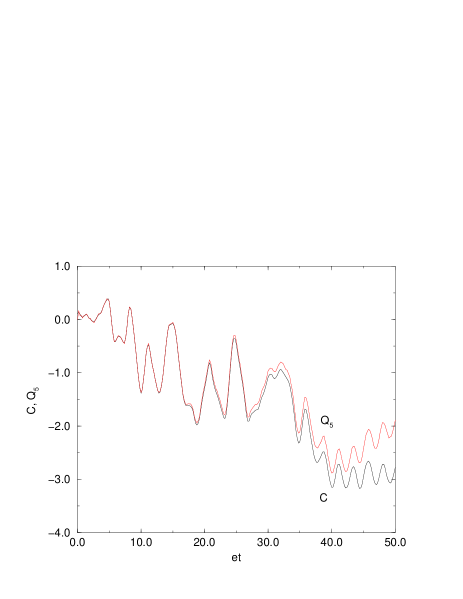
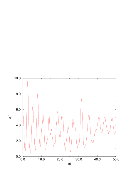
FIG. 5.: $C$ and $Q_{5}$ versus $et$.

FIG. 6.: Order parameter $|\phi|^{2}$ versus $et$.

VI Conclusions and outlook

We considered the real-time dynamics of a coupled system of classical Bose fields and a quantized fermion field, represented by generalized mode functions, on a lattice in space and time. Because of the presence of $2N$ spinor mode functions that are space dependent, the method is, especially in $3+1$ dimensions, numerically demanding.

The $1+1$ dimensional model is an excellent toy model to test the possibility of numerical calculations in a non-homogeneous, non-equilibrium context, including anomalous fermion production. A more detailed report will appear elsewhere [12].

REFERENCES

- [1] D.Yu. Grigoriev and V.A. Rubakov, Nucl. Phys. B299 (1988) 67.
- [2] D.Yu. Grigoriev, V.A. Rubakov and M.E. Shaposhnikov, Nucl. Phys. B326 (1989) 737; Ph. de Forcrand, A. Krasnitz and R. Potting, Phys. Rev. D50 (1994) 6054; J. Smit and W.H. Tang, Nucl. Phys. B (Proc. Suppl.) 34 (1994) 616; ibid. 42 (1995) 590.
- [3] W.H. Tang and J. Smit, hep-lat/9805001.
- [4] J. Ambjørn, T. Askgaard, H. Porter and M.E. Shaposhnikov, Phys. Lett. B244 (1990) 497; Nucl. Phys. B353 (1991) 346; J. Ambjørn and A. Krasnitz, Phys. Lett. B362 (1995) 97; Nucl. Phys. B506 (1997) 387; W. H. Tang and J. Smit, Nucl. Phys. B482 (1996) 265; ibid. B51 (1998) 401; G.D. Moore and N. Turok, Phys. Rev. D55 (1997) 6538; ibid. D56 (1997) 6533.
- [5] G. Aarts and J. Smit, Phys. Lett. B393 (1997) 395; Nucl. Phys. B511 (1998) 451.
- [6] D. Bödeker, L. McLerran and A. Smilga, Phys. Rev. D52 (1995) 4675; P. Arnold, D. Son, L.G. Yaffe, Phys. Rev. D55 (1997) 6264; P. Arnold, Phys. Rev. D55 (1997) 7781.
- [7] C.R. Hu and B. Müller, Phys. Lett. B409 (1997) 377; G.D. Moore, C.R. Hu and B. Müller, Phys. Rev. D58 (1998) 45001; E. Iancu, hep-ph/9710543.
- [8] F. Cooper and E. Mottola, Phys. Rev. D36 (1987) 3114.
- [9] F. Cooper, S. Habib, Y. Kluger, E. Mottola, J.P. Paz and P.R. Anderson, Phys. Rev. D50 (1994) 2848.
- [10] Y. Kluger, J.M. Eisenberg, B. Svetitsky, F. Cooper and E. Mottola, Phys. Rev. D45 (1992) 4659; F. Cooper, S. Habib, Y. Kluger and E. Mottola, Phys. Rev. D55 (1997) 6471; D. Boyanovsky, H.J. de Vega, R. Holman and J.F.J Salgado, Phys. Rev. D54 (1996) 7570; D. Boyanovsky, D. Cormier, H.J. de Vega, R. Holman, A. Singh and M. Srednicki, Phys. Rev. D56 (1997) 1939.
- [11] J. Baacke, K. Heitmann and C. Patzold, Phys. Rev. D55 (1997) 7815; ibid. D57 (1998) 6406; hep-ph/9806205.
- [12] G. Aarts and J. Smit, Real-time dynamics with fermions on a lattice, to appear.